Characterization of side-slip dynamics in Land Rover LR3 for improved high speed autonomous control

Characterization of Side-slip Dynamics in Land

Rover LR3 for Improved High Speed Autonomous

Control

by

Robert D. Truax

Submitted to the Department of Mechanical Engineering

in partial fulfillment of the requirements for the degree of

Bachelor of Science in Mechanical Engineering

at the

MASSACHUSETTS INSTITUTE OF TECHNOLOGY

June 2008

@

Massachusetts Institute of Technology 2008. All rights reserved.

A uthor ...

... :.

...

...

...

Department of Mechanical Engineering

May 9, 2008

Certified by...

John J. Leonard

Professor of Mechanical and Ocean Engineering

Thesis Supervisor

Accepted by

AUG

1 4 2008

IBR4ARw1F!

n H.

Lienhard V

Characterization of Side-slip Dynamics in Land Rover LR3

for Improved High Speed Autonomous Control

by

Robert D. Truax

Submitted to the Department of Mechanical Engineering on May 9, 2008, in partial fulfillment of the

requirements for the degree of

Bachelor of Science in Mechanical Engineering

Abstract

In this thesis, the side slip control dynamics of the Land Rover LR3 platform are examined for autonomous control. As autonomy becomes implemented in high speed safety applications, the importance of an accurate model for the vehicle becomes crucial for obstacle avoidance and emergency maneuvers. Testing on public highways under normal operation shows a slip ratio drop to 70% of the no-slip model, indicating a need for model improvement. By defining the slip ratio as a function of velocity with a slope of -0.018 ± 0.002 seconds per meter and a y-intercept of 1.23 + .04, much of this error may be reduced. While a more complex relationship may exist between the slip ratio, vehicle velocity, and the steering command, the noise and inaccuracy of the sensor prevent a more precise analysis.

Thesis Supervisor: John J. Leonard

Acknowledgments

Prof. John J. Leonard For advising and guiding me through the research process. Luke Fletcher For working closely with me to understand the vehicle and analysis

software and help conduct and record the tests. Jason Dorfman For his photography.

The MIT DARPA Urban Challenge team Whose code and hard work gave me a starting point for my research.

Contents

1 Introduction 11

1.1 Motivations for Civilian Autonomous Control . ... 11 1.2 Description of Autonomous Platform and System . ... 12

1.3 Control Algorithm ... .. ... .. 14

2 Experimental Model and Methods 15

2.1 Experimental Procedure ... 15

2.2 Vehicle Dynamic Model ... 15

2.3 Variables of Concern ... 16

3 Results and Discussion 17

4 Conclusion 23

List of Figures

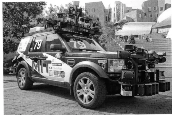
1-1 Photo taken of MIT's DARPA Urban Challenge Land Rover LR3 taken

Oct 1, 2007 by Jason Dorfman ... . 13

3-1 Plot of the slip ratio vs. the vehicle velocity for the slow speed, outgoing highway, and returning highway data. . ... 18 3-2 Plot of slip ratio vs. vehicle velocity and accompanying fits. Each fit

line corresponds to one of three sets of data. . . . . 19 3-3 A plot of slip ratio vs. velocity between all three data sets with a high

speed fit line. . . . .. .. . . .. . . . .. . 20 3-4 Plot of the slip ratio vs. the applied steering command. Note the high

noise and sensitivity at low steering commands. . ... . . . 21 3-5 Plot of slip ratio vs. vehicle velocity and applied steering command.. 22

Chapter 1

Introduction

With the government sponsorship of enormous robotic vehicle competitions, most recently the DARPA Urban Challenge, fully autonomous vehicles have been pushed into the conscience of the mainstream public. Now being designed for military appli-cations, the same technology will reach the civilian marketplace in the near future. One of the motivations and concerns for autonomous control of civilian vehicles is safety. The first computer controls may be for high speed obstacle avoidance in the case that the human driver is not aware or capable of taking evasive action. Since it is not desireable for the vehicle's computer to take control during normal operation, optimal design would only take control in the minimum time before a collision would occur. Because of the narrow time window, high speed, and extreme maneuvers re-quired, an accurate model for the dynamics of the vehicle is critical. Combined with a system to sense road conditions, such as the amount of water or snow on the road, a predictive system would be capable safe operation in real world conditions.

1.1

Motivations for Civilian Autonomous Control

According to the Fatality Analysis Reporting System, there were 38,588 fatal car crashes in 2006.1 Many of these are results of driver error resulting from drunk driving, falling asleep at the wheel, recklessness, ignorance of road conditions, distractions

due to a variety of technologies, and other influences. As roads continue to become more congested, the chances for accidents rises. While many advances in car safety have been produced over the past half century to mitigate the damage caused by car crashes to passengers, there has been very little done to address the root cause of most accidents: the drivers. The goal of autonomous control is to remove the error prone driver and replace him with a reliable, robust, and safe computer control algorithm.

Through competitions such as the DARPA Urban Challenge, it has been proven that full size computer controlled vehicles are able to safely navigate both off-road and urban terrain for military purpose. In the latest competition, vehicles even interacted with each other through 4-way stops, passing maneuvers, and in the parking lot without any prior collaboration except through the state of California driving rules.2 The only two accidents that occurred were at very low speeds and produced little or no damage. This is extraordinary because it illustrates that it is not necessary for all cars on the road to be programmed with the same algorithm, or even all autonomous at all. Through careful design, autonomous control may be implemented slowly into mainstream society safely.

Even today, some luxury car models have limited autonomy. When stopped in the correct location near a parallel parking space, the computer control may be activated and the car can parallel park itself. This marks the use of autonomy for minimal interaction with a static outside environment. One of the next steps is to have the car engage automatically in emergency situations to avoid both static and moving obstacles without the interaction of the driver. This vision for the next civilian autonomous vehicle stage is the basis for dynamic model developed in this thesis.

1.2

Description of Autonomous Platform and

Sys-tem

The platform on which the experiments were conducted for this thesis was MIT's DARPA Urban Challenge Land Rover LR3 as shown in figure 1-1. For full

Figure 1-1: Photo taken of MIT's DARPA Urban Challenge Land Rover LR3 taken Oct 1, 2007 by Jason Dorfman.

fications of the vehicle, please see appendix A.1. The vehicles has many sensors to determine its location and characterize the environment around it. For the purposes of this thesis, only factory built-in engine control unit (ECU) and the Applanix POS-LV-220 inertial navigation unit will be used. The vehicle ECU senses the steering wheel position while the Applanix measures the rotation rate and speed of the vehi-cle. The Applanix is mounted in the rear of the LR3 just forward of the rear door handle, and the software used has corrected for this offset from the center of mass.3

The factory weight of a new empty LR3 is just over 5,400 lbs, and fully loaded is expected to weigh just over 7,000 lbs. After being fully loaded with sensors, com-puters, and other equipment, the Land Rover service center estimated its weight at just under 9,000 lbs. This extra mass illustrates the importance of establishing an accurate model for high speed control, since inertial forces carry an exaggerated effect on the performance of the vehicle.

3

1.3

Control Algorithm

While the specific details of the autonomous control algorithm are complicated, only a simplified understanding is necessary. The step-by-step algorithm for planning and control follows:

1. A destination waypoint is fed into the controller.

2. A random set of possible paths forward are generated and simulated using the vehicle dynamic model.

3. The most efficient safe path forward is selected and commands are sent to the vehicle.

This process is repeated at a 10 Hz frequency during autonomous control.4 This fast update helps to mitigate errors in the model by limiting the time errors may accumu-late. However, at highway speeds, the vehicle may move as far as 3 meters between updates, making a more accurate dynamic model important, especially during emer-gency maneuvers that must be carried out in fractions of a second.

4

Chapter 2

Experimental Model and Methods

2.1

Experimental Procedure

To collect data of the vehicle at various speeds and steering commands, three test runs were conducted. The first was in an empty parking lot at low speeds and high steering commands. The driver maneuvered in various circles and speeds while the relevant data was collected. The second data set was on a 13 mile section of interstate 93. The third data set is of the return journey on interstate 93. Road conditions were good, with warm and dry weather.

2.2

Vehicle Dynamic Model

For the purposes of the DARPA Urban Challenge, the vehicle was modeled for low speed and good road conditions. Therefore, it was assumed that there would be no sideslip. To determine the expected angular trajectory of the vehicle, a simple bicycle model was used.

Omax = arctan b (2.1)

rmin

= - tan (uX Omax)

w = rx b x v (2.2)

where 0_{max is the maximum turn angle of the vehicle, b is the wheelbase, r,i,n is the}

minimum turn radius, w is the yaw rate, r is the slip ratio, u is the steering command from the driver, ranging from 0 for a centered wheel to 1 for a fully turned wheel, and v is the velocity of the vehicle.1 In the current model, r is defined as 1.

At high speeds, the no slip condition is no longer valid, and r will vary. It is assumed that r will be some function of v and u. The purpose of this thesis is to identify that relationship. While normally a simple analysis of a vehicle would include an examination of the centripetal forces and rubber wheel characteristics, the LR3's anti-rollover and stabilization software interferes with rigorous testing. Much of this implementation remains proprietary, and cannot be accounted for. Therefore, this thesis will attempt to generalize the results of all these factors into variables that are measureable and controllable, allowing a characterization without intimate knowledge of the inner workings of the vehicle.

2.3

Variables of Concern

In order to characterize the sideslip of the vehicle, this thesis will examine three main variables:

* s The steering command of the wheels, directly proportional to the wheel angle. * v The velocity of the vehicle.

* r The slip ratio, defined in equation 2.4 listed below. The slip ratio is defined as

r = actual (2.4)

Wpredicted

where Wactal is the actual yaw rate of the vehicle and Wpredictd is the yaw rate predicted

by the no-slip model of the vehicle.

Chapter 3

Results and Discussion

The slip ratio was shown to have a roughly linear correlation with the vehicle velocity and a weak correlation with the applied steering.

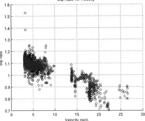
Figure 3-1 shows the correlation between the vehicle velocity and the resulting slip ratio. Note the high noise in the data at low speeds, and comparable noise at the high speeds. Since the accuracy of the Applanix is high, this noise is believed the be a result of the lower quality steering wheel sensor combined with a sensitivity in the slip ratio to small changes in the steering wheel angle. Therefore, while a precise characterization of the dynamics is difficult to attain, an overall linear trend seems to match well enough to eliminate a significant amount of the error that would arise should slip be ignored.

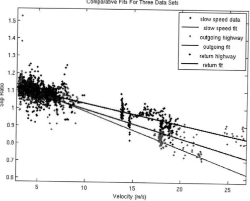
Linear fits to the same plot are shown in figure 3-2. The three fit lines represent linear fits over the three data sets. Note how the y-intercept for each exceeds 1, indicating an error in the original model of the vehicle.

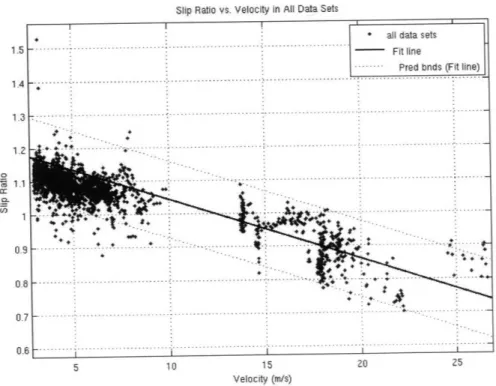
In order to find a more accurate fit for high speed, all data sets were combined and all points with velocities below 12 meters per second were removed from the fit. The resulting graph can be seen in figure 3-3 with the low velocity points shown only to help visualize the fit. This fit line has a slope of -0.018 ± 0.002 seconds per meter and a y-intercept of 1.23 ± .04 for a 95% confidence interval, which is indicated by the dotted lines. This reflects the best fit for the high speed region with which we are concerned.

Slip Ratio vs. Velocity ... . ... i ll.... ... .. . ... ... 0: 7 .. _{f ( 16 0:} ... 9 o q !... . . . . 0 ₀₀

_{8... 0 .}

Figure 3-1: Plot of the slip ratio vs. the vehicle velocity for the slow speed, outgoing highway, and returning highway data.

I .A 1.5 1.4 1.3 o 1.2 1 0.9 0.8 I m

I

I

Comparative Fits For Three Data Sets 1.5 1.4 1.3 1.2 o i7 1.1 r,-1 0.9 0.8 0.7 0.E 5 10 15 Velocity (m/s)

Figure 3-2: Plot of slip ratio vs. vehicle velocity and corresponds to one of three sets of data.

20 25

Slip Ratio vs. Velocity in All Data Sets

5 10 15 20 25

Velocity (m/s)

Figure 3-3: A speed fit line.

plot of slip ratio vs. velocity between all three data sets with a high

o

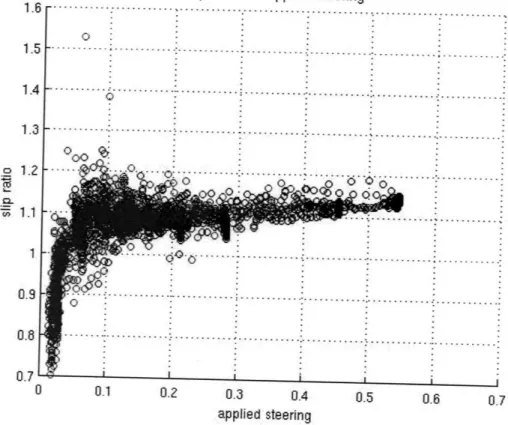
For comparison, a plot of slip ratio vs. applied steering command can be seen in figure 3-4. A weak correlation is evident for all but the lowest applied steering

com-Slip Ratio vs. Applied Steering

1.b 1.5 1.4 1.3 S1.2 n 1.1 1 0.9 0.8 0.7 ... ... ... ... . ... .. ;.. . . .. . .... . . 0 0 I-·:' · · · · · :-' · '''' L·.I-·· · · · :···

...

..

..

.

.

...

Figure 3-4: Plot of the slip ratio vs. the applied steering command. Note the high noise and sensitivity at low steering commands.

mands, while the slip ratio appears to show a high sensitivity to the steering command at low values. Due to the lower accuracy of the steering command sensor, this limits the ability to analyze the precise dynamics without high quality instruments.

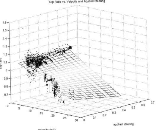
When viewed together on a three dimensional space as in figure 3-5, one can see the strong correlation between the slip ratio and vehicle velocity, while also seeing the weak correlation between the slip ratio and the applied steering. Note the lack of data for high speed and high turn rate. While this data would be useful _{for a} complete analysis of the vehicle dynamics, it is unsafe to perform these tests without trained professionals.

Slip Ratio vs. Velocity and Applied Steering 1.6 -.... .. 4 . 1.4 -. ... : . 30 0 applied steering Velocity (m/s)

Figure 3-5: Plot of slip ratio vs. vehicle velocity and applied steering 1. . . . . ' . : " : " * • . .. . . . i " . . . command.

.o ~ -•FiL "•: % •... '•• {•"" ":... ... •5 :' " M" 0;3.-:• ...i •2 0>..¢. . .,.. ' .. ... . .. .

Chapter 4

Conclusion

This data shows that at highway speeds around 25 m/s, the slip ratio drops to around 70% of the low speed value, indicating a need for an improved dynamic model. It is recommend that the slip ratio be modeled as a function of vehicle velocity by the following equation:

r = ax v +P (4.1)

where r is the slip ratio, a is -0.018 seconds per meter, and / is 1.23. The 95% confidence interval is ± 0.002 for a and ± 0.04 for 0. These relationships may be studied for various road conditions and the range of application may be expanded for civilian applications. By implementing this model, safety may be improved for autonomous control during high speed emergency maneuvers.

Appendix A

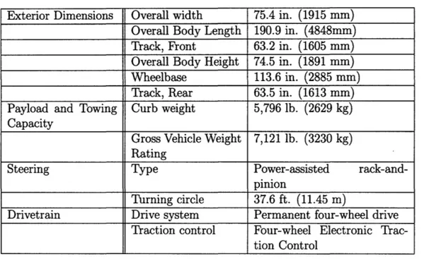
LR3 Specifications

Table A.1: Relevant specifications of Land Rover LR3. Exterior Dimensions Overall width 75.4 in. (1915 mm)

Overall Body Length 190.9 in. (4848mm)

Track, Front 63.2 in. (1605 mm)

Overall Body Height 74.5 in. (1891 mm)

Wheelbase 113.6 in. (2885 mm)

Track, Rear 63.5 in. (1613 mm)

Payload and Towing Curb weight 5,796 lb. (2629 kg) Capacity

Gross Vehicle Weight 7,121 lb. (3230 kg) Rating

Steering Type Power-assisted

rack-and-pinion

Turning circle 37.6 ft. (11.45 m)

Drivetrain Drive system Permanent four-wheel drive

Traction control Four-wheel Electronic

Trac-tion Control

Taken from Land Rover website: http://www.landrover.com/us/en/Vehicles/LR3/Overview.htm on May 7, 2008.