Publisher’s version / Version de l'éditeur:
Vous avez des questions? Nous pouvons vous aider. Pour communiquer directement avec un auteur, consultez la première page de la revue dans laquelle son article a été publié afin de trouver ses coordonnées. Si vous n’arrivez pas à les repérer, communiquez avec nous à [email protected].
Questions? Contact the NRC Publications Archive team at
[email protected]. If you wish to email the authors directly, please see the first page of the publication for their contact information.
https://publications-cnrc.canada.ca/fra/droits
L’accès à ce site Web et l’utilisation de son contenu sont assujettis aux conditions présentées dans le site LISEZ CES CONDITIONS ATTENTIVEMENT AVANT D’UTILISER CE SITE WEB.
Proceedings of the 4th International Conference on 3-D Digital Imaging and
Modeling (3DIM2003), 2003
READ THESE TERMS AND CONDITIONS CAREFULLY BEFORE USING THIS WEBSITE. https://nrc-publications.canada.ca/eng/copyright
NRC Publications Archive Record / Notice des Archives des publications du CNRC : https://nrc-publications.canada.ca/eng/view/object/?id=f018e9a6-4976-4676-95c8-741d9412c019 https://publications-cnrc.canada.ca/fra/voir/objet/?id=f018e9a6-4976-4676-95c8-741d9412c019
NRC Publications Archive
Archives des publications du CNRC
This publication could be one of several versions: author’s original, accepted manuscript or the publisher’s version. / La version de cette publication peut être l’une des suivantes : la version prépublication de l’auteur, la version acceptée du manuscrit ou la version de l’éditeur.
Access and use of this website and the material on it are subject to the Terms and Conditions set forth at
Recursive Model Optimization Using ICP and Free Moving 3D Data
Acquisition
National Research Council Canada Institute for Information Technology Conseil national de recherches Canada Institut de technologie de l'information
Recursive Model Optimization Using ICP and
Free Moving 3D Data Acquisition *
Blais, F., Picard, M., Godin, G.
October 2003
* published in the Proceedings of the 4th International Conference on 3-D Digital Imaging and Modeling (3DIM2003). October 6-10, 2003. Banff, Alberta, Canada. NRC 45834.
Copyright 2003 by
National Research Council of Canada
Permission is granted to quote short excerpts and to reproduce figures and tables from this report, provided that the source of such material is fully acknowledged.
Recursive Model Optimization Using ICP and Free Moving 3D Data Acquisition
*François Blais, Michel Picard, Guy Godin
National Research Council of Canada
Institute for Information Technology
Ottawa, Ontario, Canada, K1A 0R6
Email:
[email protected]
*
NRC-45834
Abstract
This paper describes a recursive multi-resolution algorithm that reconstructs resolution and high-accuracy 3D images from low-resolution sparse range images or profiles. The method starts by creating a rough, partial, and potentially distorted estimate of the model of the object from an initial subset of sparse range data; then, using ICP algorithms, it recursively improves and refines the model by adding new range information. In parallel, real-time tracking of the object is performed in order to allow the laser scan to be automatically centered on the object. The end result is the creation of a high-resolution and accurate 3D model of a free-floating object, and real-time tracking of its position. Examples of the method are presented when the object and the 3D camera are moving freely with respect to each other. The system provides high accuracy hand-held laser scanning that does not require complex and costly mechanical scanning apparatus or external positioning devices.
1. Introduction
Because of their inherent physical properties, 3D scanners can only measure one view of an object at a time. Therefore to completely reconstruct an object, multiple images must be acquired from different orientations. Two main solutions have been proposed to combine these different views: to use external global positioning equipment such as CMM, optical or mechanical trackers, inertial guidance systems, or to use software algorithms to merge and stitch these multiple images together. The introduction of Iterative Closest Point (ICP) registration algorithms has greatly simplified the reconstruction of complex 3D models of objects acquired using 3D scanners. In the context of this paper, the term ICP encompasses the family of Iterative Corresponding Point methods [1].
The Iterative Closest Point algorithms (ICP) have been developed mostly for solving the general problem of registration of range images acquired from multiple partial views of a same object [2]. Many variations of these algorithms have been published but basically the objective is to find the best rigid transformation matrix that maps one set of range data to a reference set. This rigid transformation can then be used to stitch a new patch image to the reference surface.
Several algorithms have been proposed to constrain convergence: minimizing the quadratic errors of the minimum distances between each point on the new patch and the reference surface (point-to-surface), between two surface patches (surface-to-surface), or between each point (point-to-point). To speed up the algorithm, the normal to the surfaces or to the segments are often used to reduce the complexity of the search. Many other methods have also been proposed: error minimization using the conventional quadratic and/or absolute errors, outlier removal, minimization of error distributions in the scanner coordinate system rather than the object [1,3,4].
Mathematically, the objective of ICP algorithms is to find the rigid transformation matrix Mk that will align the
range data set
k
x in the scanner coordinate system with the model reference image data set xmk where
k k Mkx xm = (1)
[
]
T k = x y z 1 x (2)ICP algorithms generally assume that the data within the images are rigid, accurate, and most importantly, stable during the acquisition (still images). Thus, the 3D scanning process must meet the requirement that the relative position between the scanner reference coordinate and the object under inspection is kept perfectly stable and distortions free. Unfortunately, relative motion between the scanner and the object will introduce two
undesired sources of errors: blur of the individual measurements, and overall motion-induced distortion across the scan. Very short integration time of the light on the position detector can reduce blur but distortions will still exist and will depend on the acquisition rate, processing speed of the data set
x
k, and the physical properties of the scanner.From an initial set of sparse 3D points, the method presented here estimates a rough, partial, and potentially distorted model that provides a first approximation of the expected object. This model is also used to track the position of the object in a 3D space. New profiles are added to this initial set to recursively improve and refine the initial model and to simultaneously provide object tracking information. The final result is a high-resolution accurate representation of free-floating objects.
An analogy with a sculptor can be made. He will start from a large piece of wood or granite, will progressively add outlines, and will refine the details of his masterpiece. The proposed method is similar; details are added while continuously scanning the object.
In section 2, we will discuss the most important physical constraints associated with 3D acquisition that will help defining the requirements for the algorithm. Sections 3 and 4 will present the algorithm and its implementation. Section 5 will present different scanning scenarios that we tested and the experimental results that were obtained.
2. The constraint of physical rigidity during
acquisition
Constraining the object to be rigid and stable is still a major requirement that must be maintained during the acquisition of range data. Constrained rigidity means that any motion is predictable and can be accurately computed.
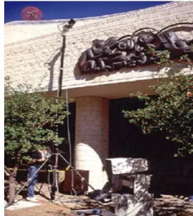
Figure 1 shows a dual-axis range sensor mounted on a tripod. The tripod is physically moved around the object to create a full 3D model. Stability is paramount in acquiring high accuracy images and will be seriously compromised by mechanical oscillations and vibrations, amplified by the length of the tripod arm. In this case the rigidity constraint between the object and camera depends on the stability of the tripod and will not be valid in the presence of strong winds, vibrations, or mechanical oscillations. The use of positioning equipment such as optical trackers is only a partial solution; an absolute mechanical rigidity between the optical tracker and the object must still be maintained. Such an arrangement would not be possible with the hand-held scanning method illustrated in Figure 2.
Figure 2 illustrates the hand-held configuration we used in this paper. Removing any constraints associated with rigidity will solve the stability problem of Figure 2 and can dramatically reduce the costs associated with mechanical structures of Figure 1, since the proposed approach works identically when the 3D scanner is being moved relative to the object, something that was Figure 1: Range sensor mounted on a tripod; stability is paramount in acquiring high accuracy range images. Accuracy of range data is the combination of the range sensor and its mechanical supporting structure. Vibrations and oscillations induced by winds or passing vehicles can seriously affect accuracy.
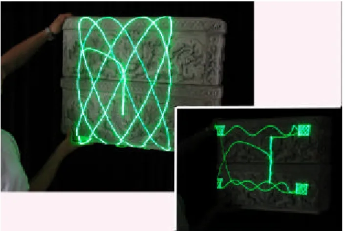
Figure 2: Hand-held acquisition using fast Lissajous scanning patterns and real-time tracking using the 3D range data. External constraints imposed in Figure 1 or by using external trackers are completed removed; no external equipment is needed. This is one of the experimental configurations we used during this work, the exactly equivalent opposite being holding the 3D camera.
successfully tested as part of this work by holding the scanner in hand.
Table 1 shows typical acquisition times needed to create high-resolution 3D images assuming an acquisition rate of 10 kHz. Mechanical stability must be guaranteed for more than 2 minutes to acquire an image of 1024×1024 rigels (Range ImaGe ELements). Even 2 seconds for a much smaller 128×128 image is still problematic in many situations involving motion.
Table 1: Typical acquisition speed using raster imaging.
Image Size (sec)
128 128 1.6 256 256 6.6 512 512 26.2 1024 1024 104.9 Acquisition rate Retrace time 10 kHz 2 ms
Table 2: Typical acquisition speed using Lissajous scanning patterns.
Pattern Size (msec) (Hz)
128 13 78
256 26 39
512 51 20
1024 102 10
Acquisition rate 10 kHz
The acquisition rate is important to characterize the maximum displacement speed of the object that can be measured and to compensate for the ever-present oscillations and vibrations, according to the Nyquist criteria. Motion is usually slow and therefore its equivalent spectrum is low in frequency content. Experience shows that mechanical oscillations in the 10 Hz to 100 Hz are expected and that higher frequencies oscillations are usually damped because of the natural inertia (weight) of the 3D camera and/or the object. Assuming an acquisition rate of 10 kHz, this means that a maximum of 100 to 1000 rigels/sec can be used for data registration without being hampered by aliasing. Unfortunately for the moment, an increase in acquisition rates, for example by sub-dividing the detector or using pattern projectors, will usually result in much reduced accuracy and/or smaller volumes of range measurement [5] and is not a practical solution.
In [6] we have demonstrated the use of Lissajous scanning patterns to obtain real-time tracking performances. Figures 2 and 3 show the use of different scanning scenarios that can be used to acquire
high-resolution accurate 3D profiles. Table 2 shows typical pattern rates that can be obtained.
3. Algorithm
Many different ICP methods have been demonstrated to compute the registration matrix between a subset of data and a reference object. In [2] the algorithm searches for the closest point to a reference surface. To reduce the search space, several authors use the normal to the surface or segment and a maximum range window to limit the total number of points tested during the computation [3,7,9]. Other methods have been developed such as projecting the point following the camera point of view [7,10]. This method accelerates the computation and is less affected by noise, and although it does not represent the physical object as well, it better represents the acquired range data. A study of the performances of some ICP methods is presented in [1]. More recently [4] uses specific attributes of range data to improve performances by constraining the pairing. This also offers the possibility of avoid slipping of unconstrained surfaces. Most ICP algorithms assume uncorrelated and uniformly distributed noise ? x, ? y, ? z, which is a correct simplification for small volumes but not correct for large volumes [6].
It is not our intention to discuss the pros-and-cons of a given ICP algorithm, for the simple reason that they fall short when time and motion induced distortions are introduced. Here we therefore consider the ICP algorithm and the model reconstruction method as a generalized function, and focus instead on the recursive correction and transformation of these data and model to be compatible with existing ICP.
Figure 3: Variations of the scanning patterns, multiple Lissajous and combined Lissajous and raster/vector imaging.
Let assume a subset X of Nk k calibrated range data
acquired by the range sensor. Each point x has an i associated time tag ti:
[
]
T z y x 1 = x (3){ }
i i k k = x;t 0≤i<N X (4)This subset corresponds to a profile or a full pattern as illustrated in Figure 3. The time tag ti is used to
compensate for motion-induced distortions. Let us assume that m is a point on the model and mˆ is an approximation of that model. The problem of registration consists of finding the estimate Rˆ of the rigid k
transformations R that minimizes the equation k
∑
− = − = 1 0 2 , ˆ ˆ ˆ k N i i i k i k k m R Dx ε (5)The selection of the point mˆ depends on the ICP algorithm. Dˆ is an estimate of the compensation matrix i
i
D that removes the residual distortions introduced by motion within the profile X . We are for now assuming k that the distortion matrix is unity, Di =I.
Let us also assume that we have a function ℑ that creates our estimate mˆ of the object from the K previous profiles or images:
(
k i i)
kk =ℑR D x ∀
mˆ ˆ ˆ (6)
The functionℑ creates a mesh model from a set of range points X . The first model k m is obviously a very rough ˆ0 estimate. The model creation procedure basically appends M new profiles to the previous model estimate mˆk−Mthat fill the gaps, expand its surface and refine the geometry of the new estimate mˆ . The final step is to re-optimize the k last model mˆ by iteratively re-evaluating the matrices k
k
Rˆ and recreate a new model estimate mˆ that will minimize the total error
∑
− = = Ε 1 0 K k k ε (7)Experimental tests show that optimization is fast and converges in a few iterations, especially if this optimization is implemented at the beginning of the optimization for a small number of subsets K, i.e.
k
k R
Rˆ ≈ for K small (8) In a practical situation the relative displacement of the scanning patterns on the object surface are usually small. The initial model estimate mˆ is only a local representation of a small patch of the complete object.
The next few profiles correct this locally distorted patch mˆ and quickly converge to a much more accurate representation of this same patch m . Subsequent profiles mostly expand an already good model (mˆ ≈m). Although Equation 7 can be used to automatically verify the convergence of Equations 5 and 6, we found that in practice a fixed number of iterations is sufficient.
Final improvements can be included in the algorithm by interpolating the estimates Dˆ of the motion distortion i
matrix D for each measurement i using a function i Ω and the rigel time tag ti of Equation 4. Motion is
interpolated from the relative trajectory of the object or scanner given by the matrices Rˆ k
i k k k i , ˆ , ˆ ,ˆ , ;t ˆ 1 1 K K − + Ω = R R R D (9)
The simplest form for Ω is a linear interpolation between the Rˆk−1,Rˆk using quaternion for the rotation,
for example. Better methods can include smoothed interpolation using Rˆk−1,Rˆk,Rˆk+1, bi-cubic
interpolations, or to include acceleration. At the time of writing this paper, we were still evaluating these different scenarios.
If K is large, the final model should be a very close representation of the exact model, that is
i i k k k m R R D D mˆ = ; ˆ = ; ˆ = (10)
4. Practical implementation
This algorithm includes three quasi-independent operations that are easily implemented in parallel using asymmetric distributed processing.
1 Tracking: from R we know the relative position of k the object from the scanner. In an open-loop system, this information can be used to update the object location on a display screen for example. In a closed-loop system, R is used to instruct the k scanner to adjust the position of the scanning pattern on the object.
2 Model creation: new profiles X are added to the k model estimate mˆ , thus expanding it. With enough scans, the entire surface of the object can be estimated. This operation is identical to the problem of multi-view registration but using only sparse data. 3 Model refinement: the model mˆ is recursively optimized using the previous profiles ∀Xk, or the ones that fit a certain quality criteria such as rigel resolution; final removal of the local distortions induced by motion can also be taken into account in the model estimate using D . i
We have already mentioned the use of Rˆ in an open-k
loop configuration such as, for example, to adjust the position of the object on a display screen Figure 5). R is k sufficient to provide the tracking information. However, in a closed loop system where the position is fed back to the scanner to track the object, delays and improper gains can easily create an unstable system resulting in overshoots or oscillations while tracking.
Closed-loop control is more complex than simply returning the position error signal. Although we will not discuss the details of implementation, a deadbeat controller is used to guaranty speed and stability [11]. A PID controller is a simplified configuration of a deadbeat controller and adjusts the proportional (error), integral (position), and differential (speed) feedback gains in relation to the physical properties of the laser scanner.
In practice ICP algorithms are unpredictable in terms of speed of convergence and therefore tracking will be jerky and slow. To provide stability, we must add a more reliable, fast, and real-time tracking mechanism; we are here using the approximate geometry of the object and fast correlation methods. The center of mass of the local geometry is often more than adequate. Possible drifts induced by these local but fast linear approximation methods will be asynchronously compensated by R . k
k
R is used to predict where the object is located, in other words to supervise the tracking. Figure 4 shows the tracking architecture. The real-time inner loop is implemented using the scanner’s QNX real-time
operating system.
From the point of view of the expanded ICP algorithm, these operations are mostly hidden except for one important physical constraint. The expected scanning position on the object may differ from the measured data, because of lags for example, and must be considered when applying the ICP algorithm. Real-time performances requirements also decrease with the complexity of a task. Asynchronous operations are possible.
The multi-tasking algorithm can be described as follows:
Task 1: acquisition and real-time tracking a) Acquire a profile Xj
b) Tracking
• Correlate profile Xjwith reference profile ref
X or reference geometry
• Send tracking error to the scanner controller system
• Update Xref =Xj
Task 2: object tracking and scanning prediction a) If reference model mˆ defined
• Find R according to Equations 5 and 6 k b) Send updated scanning position to the scanner
using R k • Set Xref =0 Task 3: object model creation
a) If reference model mˆ is not defined • Wait until tracking error (task 1) small • Use Ki profiles X and k Rˆ to create a first k
approximation of the model m ˆ0 b) If reference model mˆ is defined
• Update previous model mˆk−M with the new model estimate mˆ using all K profiles. The k asynchronous nature of this operation is illustrated by the fact that in general, M≥1, that is, the task is not necessarily performed for each new profile.
Task 4: model refinement
a) Recursively, from profiles Xjand matrices Rˆ k
• Compute better estimates of registration matricesRˆ and motion induced distortions k
matricesDˆ k
• Compute new model mˆ
b) Globally update model mˆ and matrices Rˆ and k k
Dˆ , send result to tasks 2 and 3. Laser Scanner Profile correlation and/or centroid detection Tracking error Reference Expected Object/ scan position (tracking) 3D Range Profile 3D Model ICP Dead-beat controller (tracking) Model Optimization Profile/Object Positions Motion Distortion Compensation Real-time tracking Supervised ICP tracking Model creation R e a l-ti m e Q N X N o n R e a l-ti m e W in d o w s
Figure 4: Real-time tracking consists of two feedback loops: a fast real-time linear method based on correlation and/or center-of-mass to provide stable and optimum tracking, and a non-deterministic quasi real-time supervisory loop using the proposed ICP based algorithm.
Task 1 provides real-time “smooth” control of the acquisition and tracking. Errors are usually small and processing speed is predictable and fast. This is needed to avoid loosing the object during tracking. As shown in Figure 4, Task 1 is implemented within the scanner software to remove any latencies such as those created by the communication links or the operating system. Task 2 is the result of the ICP algorithm; the estimated Rˆ k
basically supervises the tracking of Task 1 and compensates for cumulative deviations. Although still a high priority task, the asynchronous operation of Task 2 allows latency and delays created by remote processing and non-deterministic performances. These estimates
k
Rˆ are also used to expand and update the model mˆ of Task 3. Finally Task 4 is computationally very expensive and, not being part of the tracking loop, can be executed at a lower priority. To maximize speed, each task can be separately executed on a different processor.
5. Experimentation
Although many ICP algorithms can be used for Tasks 2 and 3, we used the point-to-surface method [3] implemented by Innovmetric in their PolyworksTM software package [12]. Its ease of use, versatility and reliability, make it an excellent choice for prototyping and experimentation. We intensively used the built-in macro language that simplified the testing and integration with our own software modules, as well as with the scanner. Some compromises were required to resolve implementation constraints such as the non-real time performances of the program, the Windows environment and the extensive use of files.
Integration with the laser scanner system, data transfer and command control is implemented using TCP/IP between the non-real time Windows and the real-time QNX operating system for the laser scanner. The latency and non-deterministic operations imposes the use of an asynchronous multi-tasking method such as the one we propose here.
The complete system extensively uses Lissajous scanning patterns or a combination of Lissajous, raster, and vectors. A Lissajous scanning pattern possesses many interesting opto-mechanical properties and is the best compromise between scanning speed and accuracy [13]. Most importantly in scanning moving objects, they remove the retrace time required with the more conventional raster of vector image and provide good 2D data point distribution on the object surface, needed to
avoid singularities that 1D line scan or profiles will generate in Equation 5 (not enough constraints).
6. Creation of a medium resolution model
and tracking
This first experiment demonstrates the creation of a medium resolution model m and the basic tracking ˆ0 capabilities of the algorithm. Tasks 1, 2a and 3a are illustrated in Figure 5. Here tracking task 2b is used only for display purpose and does not control the scanner.
The model of the object is at priori not known, only its overall dimensions. The system detects an object when it enters a specific volume (e.g. < 2 m) within the field of view of the scanner. The algorithm then locks on its overall geometry and positions a Lissajous pattern on its geometrical center-of-mass (Task 1). When the object motion slows and is relatively stable, a low-resolution 128x128 raster image is used to create a first model estimate m of the object. Tracking is then resumed and ˆ0 the model estimate mˆ is refined; m is distorted because ˆ0 of possible residual displacements during the 1.6 seconds needed for the initial raster image.
Figure 5: Tracking and imaging video sequence. Top-left: the system searches for an object within the field of view of the scanner; top-right: the object is found and a very low-resolution distorted model is created; left: tracking is resumed and the model refined; bottom-right: results of tracking and model creation.
Figure 6 illustrates the results of the optimization. Figure 5 shows frames extracted from the video sequence showing the tracking and the absolute display position of the object as detected by the ICP. Close scrutiny shows that the laser does not need to be perfectly centered on the object (control) to obtain accurate pose estimates Rˆ . k
Creation of a high-resolution model mˆk
This second experiment tests the creation of a high-resolution model of a larger object. Object tracking was not performed and the user manually moved the object in front and within the field-of-view of the scanner to create this complete model. This mode of operation tests the hand-held capabilities of the algorithm under user supervision.
Figure 2 shows the experimental set-up and the object used. The Lissajous pattern was moved across the surface of the object to create a complete model. We used two different seed images to create the model of Figure 8: (1) a very low resolution and highly distorted raster image as illustrated in Figure 7, (2) a single Lissajous pattern scan similar to the single pattern of Figure 2.
Figure 7 shows the low-resolution initial model using a 128×128 raster image. Figure 8 shows the final model of Figure 2. This same experiment was also performed for the object of Figure 5, and Figure 6 shows the initial,
intermediate, and final models created. Tracking and imaging are easily combined.
Tracking and high-resolution imaging
Either a single Lissajous pattern or a simple raster image can be used as a seed model m , a raster image is ˆ0 slightly more stable providing more “lock” points for the algorithm to converge but it requires that the object must be relatively stationary for a few seconds as shown in Table 1.
These experimental tests demonstrated the convergence of these algorithms and the very close representation of model mˆkand its true model m . Experimentally it seems that the remaining residual errors are mostly due to uncompensated local distortion from the fact that we assumed Dk=I.
We found that the most important key factor that affects the quality of the results is an excellent calibration of the range data and the compensation of its dynamic properties. Most scanners produce range data in the form
[
]
Tz y
x 1
=
x , which is only an approximation of the true form x =
[
x(t) y(t) z(t) 1]
T. This Figure 6: Multi-resolution model of Figure5. From theinitial low-resolution and distorted model m to the more ˆ0 refined version mˆk (respectively K=1, 20, and 200, N=128).
Figure 7: Initial model m of the object and experiment ˆ0 shown in Figure 2.
Figure 8: Final model optimized using multiple Lissajous patterns, K= 4000, N=128.
approximation is valid because the scanner is used in static mode. Dynamic calibration implies that the range data must be converted in the form of Equation 3 and that the correlation with time associated with each 3D point x(t) be removed, or at least minimized. The time stamp ti
becomes and independent variable, uncorrelated with respect to x, y, and z.
7. Conclusion
This paper has presented a recursive optimisation method that, when combined with sparse range data, can produce high quality, high-resolution range images. The algorithm first creates a very rough and distorted model of an object and recursively optimises it using new range information and a standard ICP algorithm. The method was tested and integrated with a single spot laser scanner. Real-time tracking of free moving objects while creating high-resolution images was demonstrated providing a truly high-accuracy hand-held 3D laser scanning system.
The main objective and use of this method is, when combined with a laser scanner, to create high resolution, accurate 3D models of objects without requiring complexes and expensive mechanical structures. Examples of hard to reach objects and situations where the application cannot afford such complex mechanical setups are numerous; for example it is impossible to be stable on scaffoldings or in ladders when scanning detailed façades of historical buildings or when the sensor is mounted on the tip of a long robotic arms (e.g. Canadarm). Very interesting is also the possible use of this 3D scanner and method when mounted on a remotely operated vehicle that freely moves around the object under inspection without touching it.
Many other interesting applications can benefit from components of these algorithms such as real-time tracking and inspection of known CAD objects or using region of interest (ROI) of an object. For example, it is straightforward to replace the estimate mˆ by the real k model m , tasks 3 and 4 are then no longer needed.
8. Acknowledgments
The authors would like to thank their colleagues Louis-Guy Dicaire, Luc Cournoyer, Steve Williams, and Louis Borgeat for their helpful support. We want also to acknowledge the contribution of PRECARN and Neptec for funding.
9. Reference
1. S. Rusinkiewic, M.Levoy, “Efficient variant of the ICP algorithm”, Proc. 3DIM 2001, 145-152, 2001. 2. P.J.Besl, N.D.McKay, “A method of registration of
3D shapes”. IEEE Transactions on Pattern Analysis and Machine Intelligence, 14(2), 239-256, Feb. 1992. 3. R. Bergevin, M.Soucy, H.Gagnon, D.Laurendeau,
“Towards a general multi-view registration technique”, Trans. PAMI, 18(5), 1996.
4. G.Godin, D.Laurendeau, R.Bergevin, “A method for the registration of attributed range images”, Proc. 3DIM 2001, 179-186, 2001.
5. P. Hébert, “A self-referenced hand-held range sensor”, Proc. 3DIM 2001, 5-12, 2001.
6. F.Blais,J.-A.Beraldin,S.F.El-Hakim, L.Cournoyer, “Real-time geometrical tracking and pose estimation using laser triangulation and photogrammetry”, 3DIM 2001,205-212, 2001.
7. O.Jokinen, "Area-based matching for simultaneous registration of multiple 3D profile maps”, Computer Vision and Image Understanding, 71(3), 431-447, Sept. 1998.
8. Y.Chen, G. Medioni, “Object modeling by registration of multiple range images”, Image and Vision Computing, 10(3), 145-155, April 1992. 9. G.Godin, M.Rioux, R.Baribeau, “Three-dimensional
registration using range and intensity information”, Proc. SPIE, vol.2350, Videometrics III, 279-290, 1994.
10. G.Blais, M.D.Levine, “Registering multiview range data to create 3D computer objects”, IEEE Transactions on Pattern Analysis and Machine Intelligence, 17(8), 920-824, Aug. 1995.
11. C.L.Phillips, T.H. Nagle, “Digital Control System, Analysis and Design”, Third Edition, Prentice Hall, 1995.
12. http://www.innovmetric.com
13. F.Blais, J.-A.Beraldin, L.Cournoyer, I.Christie, K.Mason, S.McCarthy, C.Goodall, “Integration of a tracking laser range camera with the photogrammetry based space vision system”, Proc. Acquisition, Tracking and Pointing XIV, SPIE 4025, 219-228, 2000.