Simulation of dynamically structured systems in a model-based system engineering approach applied to reconfigurable hardware

HAL Id: tel-01938154

https://hal.laas.fr/tel-01938154

HAL is a multi-disciplinary open access archive for the deposit and dissemination of sci-entific research documents, whether they are pub-lished or not. The documents may come from teaching and research institutions in France or abroad, or from public or private research centers.

L’archive ouverte pluridisciplinaire HAL, est destinée au dépôt et à la diffusion de documents scientifiques de niveau recherche, publiés ou non, émanant des établissements d’enseignement et de recherche français ou étrangers, des laboratoires publics ou privés.

model-based system engineering approach applied to

reconfigurable hardware

Min Zhu

To cite this version:

Min Zhu. Simulation of dynamically structured systems in a model-based system engineering approach applied to reconfigurable hardware. Computer science. Université Toulouse 3 Paul Sabatier (UT3 Paul Sabatier), 2018. English. �tel-01938154�

THÈSE

THÈSE

En vue de l’obtention du

DOCTORAT DE L’UNIVERSITÉ FÉDÉRALE

TOULOUSE MIDI-PYRÉNÉES

Délivré par :

l’Université Toulouse 3 Paul Sabatier (UT3 Paul Sabatier)

Présentée et soutenue le 1/10/2018 par :

Min ZHU

Simulation de systèmes à structure dynamique dans une

approche d’ingénierie système basée modèles appliquée au

matériel reconfigurable

JURY

M. Vincent ALBERT Université Toulouse III Examinateur

M. Clément FOUCHER Université Toulouse III Directeur de thèse

Mme. Claudia FRYDMAN Université Aix-Marseille III Rapporteuse

M. Fabrice MULLER Univesité Nice Sophia Antipolis Examinateur

M. Alexandre NKETSA Université Toulouse III Directeur de thèse

M. Sébastien PILLEMENT Université de Nantes Rapporteur

École doctorale et spécialité :

EDSYS : Informatique 4200018

Double mention :

EDSYS : Systèmes embarqués 4200046

Unité de Recherche :

Laboratoire d’analyse et d’architecture des systèmes

Directeurs de Thèse :

Monsieur Clément FOUCHER et Monsieur Alexandre NKETSA

Rapporteurs :

same problem, and each doing his little bit to add to the great structure of knowledge which is gradually being erected.

Acknowledgements

This thesis represents the final report of my time spent at System Engineering

and Integration team of Crucial Computing department at Laboratory for Analysis and Architecture of Systems, Toulouse. I would like to take the opportunity to thank many of the people who have supported this thesis and influenced the creation of this work.

I am deeply grateful to Prof. Alexandre NKETSA, for his open-mindedness and critical advice during the discussions. I am very thankful to Clément FOUCHER, for giving constructive guidance thoughout and being an exem-plar of a professional researcher. I also would like to specially thank Vincent ALBERT, for passing on his wisdom during the model construction. Their help and supervision made this piece of work possible.

I give full appreciation to Prof. Claudia FRYDMAN and Prof. Sébastien PILLEMENT, for their interest in my work and for refereeing this thesis.

I would like to thank to Philippe ESTEBAN, who took me into this ad-venture of scientific research after my Master studies of real-time system en-gineering and stood by me during my three years teaching assistance work. Thank to Hamid DEMMOU for his team leads which make my international presentation possible. Thanks also to Claude BARON for her excellent team building.

I would like to thank all my colleagues at faculté sciences et ingenierie at université Paul Sabatier. Thanks to Emmanuel Montseny for all the prepa-ration made for the practice of Matlab/Simulink. I have shared lots of good moment with the others, especially thanks to the every year Circus.

I would like to give a special thanks to Hélène THIRION, Christèle MOUCLIER, Layla MOURCHID and Catherine GUERIN for their ongoing administrative support and for always giving a helping hand.

This thesis would not be possible without the support of families and friends, without the happiness they brought, sharing cafe culture, music, and good times spent outside of research in Finland, in Mexico, in Portugal, in China. Thank you for your great efforts people around me! Sylvain, David, Diego, Xue Rui, Karla, Guillaume, Yi Xin, Lily, Sangeeth, Yassine, Adina, Daniel et Julie, Violaine et Rémi, He Yun, Wang Rui, for all your emotional support and just being there when I need you.

In the end, I would like to give some very special thanks to the interna-tional exchange program ERASMUS, with whom I finished my undergraduate studies in France, and without whom I could not have achieved what I have today.

the need for a proper model to describe its behavior emerges. Most academic and industrial tools available on the market does not address dynamic struc-ture modeling. The arising of discrete-event modeling, in particular, Discrete Event System Specification (DEVS), propose formal tools for representing and simulating models. DEVS has already extension which handles the dynamic structure modeling. However, the capacities of these existing formalism have limitations. Notably, they do not address the components context aspect.

Also, the existing formalisms have not integrated the system engineering approach. System engineering brings beneficial procedures, notably model-driven architecture which proposes to separate the system description from its execution target. A specific model is formed from a platform-description model coupled with a platform independent model.

To address these needs, we propose a model description formalism which takes into consideration these two aspects: dynamic structure modeling and system engineering. This formalism is based on DEVS and called Partially Reconfigurable Discrete Event System Specification (PRDEVS). PRDEVS al-lows to represent dynamic-structure models independently from the simulation platform.

The presented approach can be applied to different types of targets, such as software and reconfigurable hardware. This thesis addresses these two kinds of platforms, demonstrating the suitability of the abstract formalism to actual platforms.

Keywords:

embarqués, le besoin d’un modèle de description capable de représenter ces comportements émerge. La plupart des outils disponibles sur le marché, tant académiques qu’industriels, ne prennent pas en compte la modélisation des systèmes à structure dynamique. L’émergence de la modélisation à évène-ments discrets, notamment Discrete Event System Specification (DEVS), pro-pose des outils formels pour représenter et simuler des modèles. DEVS propro-pose déjà des extensions capable de prendre en compte la modélisation à structure dynamique. Néanmoins, les possibilités offertes par ces extensions rencon-trent certaines limites. En particulier, elles ne proposent pas de moyen de gérer l’aspect contexte des composants.

De plus, les formalismes existants n’ont pas intégré l’approche ingénierie système. L’ingénierie système met en place des procédures intéressantes, no-tamment l’architecture dirigée par les modèles, qui propose de séparer la de-scription du système de sa plateforme d’exécution. Un modèle spécifique à une plateforme est ainsi la résultante d’un modèle de description de la plateforme combiné avec un modèle d’application indépendant de toute plateforme.

Pour répondre à ces besoins, nous proposons un formalisme de descrip-tion de modèles prenant en compte ces deux aspects : la modélisadescrip-tion à structure dynamique, et l’ingénierie système. Ce formalisme est basé sur DEVS, et nommé Partially Reconfigurable Discrete Event System Specifi-cation (PRDEVS). PRDEVS permet de représenter les modèles à structure dynamique indépendamment de la plateforme de simulation.

L’approche présentée peut être appliquée à différents types de cibles, tels le logiciel et le matériel reconfigurable. Cette thèse présente des mises en œuvre du formalisme abstrait sur ces deux types de plateformes, démontrant ainsi sa capacité à être déployé sur des plateformes réelles.

Mots clés :

Introduction 1

1 Scientific context & state of the art 7

1.1 System engineering and simulation . . . 9

1.1.1 Systems and system engineering . . . 9

1.1.2 Modeling and simulation . . . 11

1.1.3 Model-Driven Architecture . . . 12

1.1.4 Syntax and semantics . . . 13

1.2 DEVS and its extensions . . . 14

1.2.1 Discrete Event System Specification . . . 14

1.2.2 Dynamic Structure DEVS and its parallel version . . . 18

1.2.3 Dynamic DEVS and its dynamic port extension . . . . 23

1.2.4 Synthesizable DEVS . . . 26

1.2.5 Reconfigurable DEVS . . . 27

1.3 Dynamically reconfigurable computing systems . . . 29

1.3.1 Programmable logic device . . . 30

1.3.2 Partial reconfiguration . . . 31

1.4 Conclusion . . . 33

2 Partially Reconfigurable Discrete Event System Specification 35 2.1 PRDEVS meta-model syntax . . . 36

2.1.1 PRDEVS abstract syntax . . . 36

2.1.2 Root PRDEVS component . . . 37

2.1.3 Coupled components . . . 38

2.1.4 Atomic components . . . 38

2.1.5 Ports . . . 39

2.1.6 Convenience sets and notations . . . 39

2.2 PRDEVS semantics . . . 40

2.2.1 General functions . . . 41

2.2.2 Structure change semantics . . . 42

2.2.3 Components context under dynamic behavior . . . 44

2.3 Graphic representation . . . 45

2.3.1 Components . . . 46

2.3.2 States, transitions and actions . . . 47

2.4 Example . . . 47

3 A software PDM for the PRDEVS PIM 53

3.1 Platform study . . . 54

3.1.1 Software platform and object-oriented programming . . 55

3.1.2 A quick look into a software simulator core . . . 55

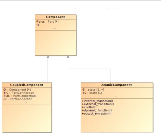
3.2 Hierarchy of the software PDM . . . 60

3.2.1 Atomic/coupled component . . . 60

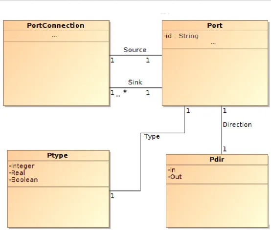
3.2.2 Port/connector . . . 61

3.3 Mapping and realization of the PDM . . . 62

3.3.1 Meta model transformation for time . . . 64

3.3.2 Input/output message bags . . . 64

3.3.3 Dynamic functions calls . . . 65

3.3.4 Time advance (Ta) . . . 65

3.3.5 Imminent time (Tn_min) . . . 65

3.3.6 Last event time (Tl) . . . 66

3.3.7 Elapsed time (e) . . . 66

3.4 Case study: a PSM test . . . 67

3.4.1 Initialization of the model . . . 69

3.4.2 Simulation . . . 70

3.5 Conclusion . . . 70

4 An hardware FPGA PDM for the PRDEVS PIM 73 4.1 PDM architecture: a high-level view . . . 74

4.2 Scheduling and temporal aspects . . . 78

4.3 Components interface . . . 79

4.3.1 Control interface . . . 79

4.3.2 Communication interface . . . 81

4.3.3 Dynamic functions calls . . . 82

4.3.4 Multi-bus . . . 84

4.4 Atomic component behavior specification . . . 84

4.4.1 FSM general structure . . . 85

4.4.2 FSM representation of internal transitions . . . 86

4.4.3 FSM representation of external transitions . . . 87

4.4.4 FSM representation of output emission . . . 88

4.4.5 Conflict . . . 89 4.5 SC functions implementation . . . 90 4.5.1 Static coordinator . . . 91 4.5.2 Dynamic coordinator . . . 92 4.6 Example . . . 93 4.7 Conclusion . . . 96 Conclusion 99

1.1 MDA structure of a meta-model . . . 12

1.2 A DSDEVS exemple: block diagram of a node . . . 20

1.3 A DSDE exemple: one server network change to two sever net-work . . . 21

1.4 A RecDEVS exemple: add a new component . . . 28

1.5 Von Neumann architecture . . . 29

1.6 FPGA architecture . . . 31

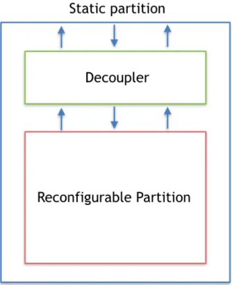
1.7 Virtual socket containing a decoupler . . . 32

2.1 Graphic representation of components . . . 46

2.2 Graphic presentation of transitions . . . 47

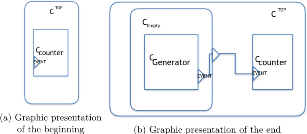
2.3 Graphic presentation of the top level component . . . 49

2.4 Graphic presentation of the generator . . . 50

2.5 Graphic presentation of the counter . . . 50

3.1 MVC Process . . . 56

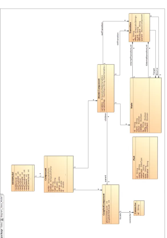
3.2 Class diagram of Model package . . . 57

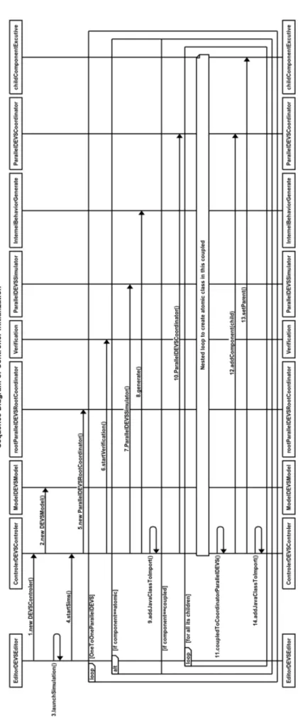
3.3 Sequence diagram of controller initialization . . . 59

3.4 PRDEVS UML representation . . . 60

3.5 Components UML representation . . . 61

3.6 Port and PortConnection types UML representation . . . 62

3.7 One-to-one correspondence . . . 63

3.8 Time variable in the different objects . . . 64

3.9 Moving Rules for players . . . 68

3.10 External view of chicken . . . 68

3.11 Internal view state machine of chicken . . . 69

3.12 Example of a game turn . . . 69

3.13 Tree view of model . . . 70

4.1 Global view of PSM . . . 75

4.2 Example of addComponent into the circuit . . . 76

4.3 Architecture of a new component added . . . 76

4.4 Example of a connection change . . . 77

4.5 Architecture of a connection change . . . 78

4.6 General simulation cycle . . . 79

4.7 Example of communication between two components . . . 80

4.8 Messages exchanges between component and coordinator . . . 81

4.10 Input X . . . . 82

4.11 Ouput Y . . . . 82

4.12 Connections between components . . . 82

4.13 Dynamic calls extra ports . . . 83

4.14 Wave of a cycle of Step . . . 84

4.15 Multi-bus structure . . . 84

4.16 General state machine . . . 85

4.17 DEVS model of an internal transition . . . 86

4.18 Internal transition . . . 87

4.19 DEVS model of an external transition . . . 87

4.20 External transition . . . 88

4.21 DEVS model of an output emission . . . 88

4.22 Output emission . . . 89

4.23 Non-conflict transition . . . 89

4.24 Conflict transition . . . 90

4.25 DEVS model of a structure change emission . . . 90

4.26 Dynamic transition: addComponent . . . 91

4.27 Coordinator . . . 91

4.28 Graphic presentation of the example . . . 96

4.29 Graphic presentation of the generator . . . 96

Mankind has created tools of all kinds to accomplish those tasks which are difficult to achieve directly by our own hands. The ambitions of human beings, together with these technologies, make it possible to fly and travel into space. However, the creation of a new system is generally not as straightforward as it might seem.

Human-made systems, from vehicles to satellites, interact with their en-vironments. The interactions between a system and its surrounding lead to different additional performance factors. The environment impacts the system properties. At the same time, the system can change its environment. For example, aircrafts lift comes from the air and the acceleration of the aircraft is limited by the air resistance at the same time. Building a system requires a full-scale consideration of all such possible interactions.

Nowadays, the creation of an artificial system is sometimes so complex that it involves interdisciplinary expert cooperation. Such a complexity makes it difficult to estimate the delays, the costs, and even feasibility. Moreover, the development of a new product can take several years. A bigger team and a longer process add complexity to a project. New methods are required to adapt to this situation, notably to identify and improve common practices that exist across the development of a wide variety of systems. A double verification or a cross-validation alone is not enough to guarantee the success of a complex project.

Verification and validation are done throughout the creation of a new prod-uct. However, there can be multiple iterations over the process, and creat-ing a product prototype each time for the verification adds to the cost and timescale. For example, a printed circuit board can take more than a week to be delivered. A verification of the virtual product using computer simulation has advantages in terms of cost and time. Lower costs and/or faster results make simulation an interesting tool for engineers. Thus, simulation is a major verification and validation method applied to the product lifecycle.

A simulation is generally done on a digital processing unit, e.g. a processor, and thus requires a digital model. A model is a representation of an actual object with a certain level of precision. Following the product engineering process, the simulation model is then an abstraction of the functions which are concerned. Moreover, a model level of representation depends on the underlying formalism. Using a very formal meta-model allows for precise and verifiable models.

Motivations

Formal meta-models consist in providing a mathematically-based syntax, a comprehensive semantic. Doing so enforces replicable simulations given the same models and an identical initial state.

Discrete event simulation is a paradigm in which the temporal evolution of the simulation is led by the events. In such a simulation, events are identified by the time in future at which they are meant to happen. This contrasts with discrete time simulations, in which the time advance is fixed and steady.

Discrete event simulation has advantages in certain cases over discrete time simulation. For example, for a system in which the time constant varies from long times to very short times. In such a case, the time step chosen can be very small to be able to account for fast variations, but this will trigger unnecessary computations for steady periods. On the other hand, if the time step chosen is longer to accelerate the simulation, one can miss fast variations which can occur between two computation slots. A discrete event simulation is able to use the derivative of the variable to determine the time of next event, so intervals are set according to the rate of change.

Formalisms like Discrete Event System Specification (DEVS) allow us to modeling discrete event systems. DEVS has a formal syntax, mathematically verifiable, and strict algorithms for simulating these models. Moreover, DEVS allows for model assemblies, which are required to build complex systems and is closed under coupling, i.e. a component made of sub-components exter-nally exhibits a behaviour which can be represented by an atomic component. DEVS is thus a strong formalism for building simulations of complex systems using a discrete event paradigm.

But when it comes to representing dynamic structure systems, DEVS ex-tensions related to such systems have limitations. DEVS formalisms for dy-namic structure systems mostly rely on predetermined architectural states. Each of these states represents a model architecture, containing components and links between components. When a transition function is triggered, the model switches from one architectural state to another. The simulation en-vironment is then responsible for inferring the actual simulation architecture from the state evolution.

While in many cases this will be enough to represent a dynamic structural system, there are other cases in which this will be a limitation. An example of this might be multi-agent systems, such as population simulation, in which agents can be born or die at some point in the simulation. In such cases, there is no way of knowing all possible architectural states of the system before simulation. We rather require a way of representing agent creation and deletion from the system, as well as relationship evolution between agents,

directly in the formalism. Another field of application is complex adaptive systems, in which the network of interactions between components of the system evolve and is able to reach net structures impossible to predict.

Moreover, having a strict approach always leads to better results. The system engineering approach provides several tools for better handling system creation, including the simulation steps. One interesting concept of system engineering is the model-driven architecture approach. Initially created for software design, model-driven architecture consists of separating the applica-tion design from the execuapplica-tion platform. It means that the applicaapplica-tion must be written using a platform-independent representation, and must incorporate a transformation tool able to generate an executable application for various platforms. This requires a high-level, platform-agnostic, model of the system and models of the platforms that will constitute the execution target. Then, by establishing a correspondence of the models, we establish a model that is able to run on a specific platform.

Among execution platforms, we usually find the classic software processors, nowadays constituted of multiple execution cores. Recently, enthusiasm for even more parallel platforms such as graphics processing units has arisen. This kind of device, initially designed for graphics applications where the same treatment must be operated on multiple pixels, has gained a general purpose use over recent years. When application speed and/or current consumption is critical, building an Application-Specific Integrated Circuit (ASIC) is also worth considering. ASICs consist in creating a logic circuit which realizes the exact function required, allowing for very important optimizations compared to software, which requires generalisation. However, the significant of fixed costs of such devices only makes them suitable for mass production.

In the middle of all theses lie Field-Programmable Gate Arrays (FPGAs). Not as fast as ASICs, not as flexible as processors, but faster than processors and more flexible than ASICs. The FPGA represents a very interesting execu-tion target for applicaexecu-tions that can benefit on-demand parallelism. FPGAs being reprogrammable logic circuits, they also benefit from unique features such as partial dynamic reconfiguration. This features consists in modifying a portion of the circuit while the remaining part continues to operate, incarnat-ing the concept of dynamic structure change. However, partial reconfiguration of FPGAs is still lacking formal methods for handling it.

Definition of objectives

At the time of writing, dynamic structure systems are new to modeling and simulation, and often treated without a clear methodology. They could benefit

from of a system engineering approach. In this work, we are aiming to define a formal modeling approach to represent and simulate dynamic structure sys-tems. To do so, we are going to formalize the representation of such systems into a meta-model. We will particularly focus on discrete-event models, and adopt a model-driven architecture approach.

As a first step, the meta-model, in other words, the model of the models must be defined. We need the meta-model to use the strong fondation of mathematical formalism. Moreover, we want the models we define to be free from constraints related to the execution platform. However, the definition must include the capability for dynamic structure change, which will restrict the available target platforms.

We also need to distinguish the dynamic structure behaviour from a model state evolving or being changed over time. The structure change takes place at a different level than the state change. Different components can exist in a system at one time, and exhibit the exact same internal behaviour while being in a different state. The state of the components thus represents an indepen-dent information set, which must be treated separately from the structure change.

The structure itself contains two levels of possible changes. A model struc-ture is composed of components, which have relationships with each other. The change can be operated either on components or on connections. We will see that this differentiation has an impact on the way it is handled by the execution platform.

Concerning the components state management, it will be useful to develop the capacity to save the state of a component during simulation, or to force it into a specific state. For example, we should be able to save the current state of a component about to be deleted so that it can be restored later. Or, a component can be instantiated with different initial states depending on the general simulation state at the simulation time.

Thus, we should study different target platforms in order to understand their execution behaviour. This will enable us to make the connection between models expressed in the developed meta-model and the platforms. We will begin with a software platform as a first target. On a software platform, many constraints are flexible, such as the memory size which, to some extent, can be ignored. During this integration period, the system engineering approach will be validated for our meta-model.

As a final objective, the meta-model should be integrated into a dynamic hardware platform. With this specific platform, the constraints (space and time) of the platform should be defined. On such a level, the communication protocol and scheduling behaviour of the simulation should have been consid-ered. The parallel nature of the platform must have been developed within

our meta-model.

Structure of the document

In this thesis, we propose an interdisciplinary work between system engineer-ing and modelengineer-ing & simulation. The scientific context and state of the art are presented in the first chapter. It details the approach of system engineer-ing and modelengineer-ing, especially for discrete event simulation and dynamically reconfigurable computing systems.

In chapter two, we propose a dynamic structure meta-model: Partial Re-configurable Discrete Event System Specification. We detail the meta-model syntax and semantics. We present the syntax using a mathematic description at a theoretical level. Then a graphic representation of the syntax is discussed to facilitate model representation.

In the third chapter, a software platform, with object-oriented program-ming, is presented to support the execution of models. We introduce a simu-lator which is able to run models described using the meta-model defined in chapter two.

In the fourth chapter, a hardware platform specification based on FPGA is presented. The platform architecture is defined in order to match the FPGA constraints.

Finally, we draw conclusions from the results and bring future perspectives into consideration.

Scientific context & state of the

art

Contents

1.1 System engineering and simulation . . . . 9 1.1.1 Systems and system engineering . . . 9 1.1.2 Modeling and simulation . . . 11 1.1.3 Model-Driven Architecture . . . 12 1.1.4 Syntax and semantics . . . 13 1.2 DEVS and its extensions . . . . 14 1.2.1 Discrete Event System Specification . . . 14 1.2.2 Dynamic Structure DEVS and its parallel version . . . 18 1.2.3 Dynamic DEVS and its dynamic port extension . . . . 23 1.2.4 Synthesizable DEVS . . . 26 1.2.5 Reconfigurable DEVS . . . 27 1.3 Dynamically reconfigurable computing systems . . . 29 1.3.1 Programmable logic device . . . 30 1.3.2 Partial reconfiguration . . . 31 1.4 Conclusion . . . . 33

System engineering consists in a process with several steps. The final goal of system engineering is to avoid failures while building a system. A complex system is usually decomposed into sub-systems, which are developed separately. The well-known V-model system engineering cycle, for example, begins with the feasibility study and concept exploration. It progressively goes down by breaking the system into sub-systems, which are fully specified individually. Finally, it ascends by testing system components and assembling them to form a complete system.

During the design of a system, modeling and simulation takes an important place. When a system is made of various sub-systems, all of them must be modeled as stand-alone pieces and tested individually. When bringing them together to form the whole system, how to co-simulate the independent models together is a really complex task. Co-simulation can happen between different types of models: hardware/software, continuous/discrete, electronic/digital, etc. It can also be done between different abstraction levels.

For classic systems, where the physical materials can be modeled, a soft-ware component can represent formally the physical materials. Before the simulation, an offline verification (static program analysis) is possible for the software components. The offline verification can be done using formal lan-guages syntactically representing the system. Before the simulation, formal methods are used as critical tools for system verification, which guarantee mathematically the system is correct. If an error is detected during the static analysis with formal methods and debug, an accident can be avoided.

The simulation is not limited to dig into the inner behavior of the system. It also looks at the interaction with a surrounding environment. In order to correctly test the system, we need to put it into its environment. It can be done by modeling the environment and simulating it together with the system. Or more directly, we can put the simulated system directly in contact with the real environment. When the system is in the real environment, the simulation must respect real-time.

For a real-time system, the actuators, physical system, and its sensors can be involved as simulated elements or as real elements in the model. As an ex-ample an aircraft stress test for its wings can contain both virtual subsystems and real subsystems. The virtual subsystem may include the control system, and the real subsystem is the airplane wing. A common practice is to model the real actuators together with the simulated physic system and sensors.

What we are interested in is dynamic structure systems, where the compo-sition can change over time. FPGA is an integrated circuit which can change its configuration to form various logic circuits. A custom design is thus pos-sible depending on the project. Moreover, some classes of FPGA are capable of run-time re-configuration during the execution.

In this chapter, we are going to discuss three main topics: system engi-neering together with model-based system engiengi-neering in section 1.1, Discrete Event System Specifications and its extensions in section 1.2, and reconfig-urable computing systems, especially Field-Programmable Gate Arrays (FP-GAs) in section 1.3.

1.1

System engineering and simulation

In this section, we will define topics of expertise which are required for the further developments. First, we will give a definition of what is a system and clarify the system engineering process. Then modeling and simulation as a part of the system engineering process will be presented. Model-driven architecture is detailed later as a system engineering approach for the software development. At last, the syntax and semantics modeling notions are defined.

1.1.1

Systems and system engineering

There are lots of definitions of what is a system. An earlier definition was done in the 50s by Ludwig von Bertalanffy [Von Bertalanffy 1956], who contributed to general systems theory. Von Bertalanffy outlines systems inquiry into three major domains: Philosophy, science, and technology:

“The systems view is a world-view that is based on the discipline of SYS-TEM INQUIRY. Central to systems inquiry is the concept of SYSSYS-TEM. In the most general sense, a system means a configuration of parts connected and joined together by a web of relationships. The Primer Group defines the system as a family of relationships among the members acting as a whole.” Here, a system is defined as elements in standing relationship.

The International Council on Systems Engineering (INCOSE) is an orga-nization aiming at improving the systems engineering practices and education developed in 1995. Their definition is straightforward:

“A system is a construct or collection of different elements that together produce results not obtainable by the elements alone.”

A system is never with only one element inside, which mean there is a possibility to decompose the system into subsystems or include a system into a larger system.

For systems engineering, the INCOSE concept is practical and includes the concept of business:

“Systems Engineering integrates all the disciplines and specialty groups into a team effort forming a structured development process that proceeds from concept to production to operation. Systems Engineering considers both

the business and the technical needs of all customers with the goal of providing a quality product that meets the user needs.”

The French association of systems engineering (AFIS) gives a definition oriented toward industrial manufacture:

“The control of complex systems by manufacturers is essential to maintain and improve the positions of French and European industry in the global mar-ket for large systems, whatever the field: transport, space, defense, finance, security, health, energy... These systems involve many disciplines: mechani-cal engineering, electrimechani-cal engineering, automatic engineering, civil engineer-ing, software engineerengineer-ing, electronic engineerengineer-ing, chemical engineerengineer-ing, indus-trial engineering, subcontracting, production, maintenance, security... but also trade, marketing, customer relations, human factors sustainable develop-ment.”

For sure, applying the system engineering concept to a complex system is interesting to ensure the success of the project. Rather than the quality, cost, delivery (QCD) approach which evaluate the results, system engineering focuses on the whole project procedure, internal communication and organi-zation.

The well-known V-model development got this name by its V form and the final steps of its procedure: verification and validation. Even though recently a lot of projects are applying other methods such as waterfall model [Bal-aji 2012], spiral model [Boehm 1988], agile methods [Ambler 2004], etc.

Within the V-model development, reliability of the system is often done by modeling and verified by simulation. It can be a general model without coding, in some case done by experience and success stories. During the requirements and architecture step, a system with several subsystems is built. Detailed designs with each subsystem’s specification are defined. Before the project moves to implementation, high-level modeling is already done.

After the implementation, during test and integration, simulation is done with different methods to ensure the subsystem is functional. Under system level verification and validation, the entire system is executed, analyzed and simulation is done on the entire system level.

The Model-Based System Engineering (MBSE) [Estefan 2007] concept was introduced by AW Wymore in 1993. It was popularized by INCOSE when it kicked off its MBSE Initiative in January 2007 [Friedenthal 2007]. The main idea is to replace the document exchange during systems engineering by creating and exploiting domain models [Friedenthal 2007].

1.1.2

Modeling and simulation

Modeling is building an abstraction of the real world, where changes of certain parameters are used to learn the way the system behaves. Simulation is based on a model which is built based on a real system, already existing or in the design phase. It shows the results by observing the model changes over time or in response to its environment.

As for the methodology for modeling and simulation, originally presented in 1976 [Zeigler 2000], it consists of two principal aspects:

Level of system specification - These are the levels at which we can

describe how systems behave and the mechanisms that make them work the way they do.

M &S sets four levels of system knowledge :

Level Name What we know at this level

0 Source What variables to measure and how to observe them 1 Data Data collected from a source system

2 Generative Means to generate data in a data system

3 Structure Components coupled together to form a generative system

Systems specification formalisms - These are the types of modeling

styles, such as continuous or discrete, that modelers can use to build system models.

A discrete system is one in which the state variables change only at a discrete set of points in time. A continuous system is one in which the state variables change continuously over time.

Under system theory [Zeigler 2000], structure – the inner constitution of a system – and behavior – its outer manifestations – are considered separately. For a time-based system, behavior and structure are connected by time-related parameters: the internal structure of a system includes its state, how one state transits to another state and the mapping between state and output. A well-defined structure helps to analyze and simulate its behavior.

Basic system concept considers the system as a black box, where we observe the output changing in reaction to the input event. After analysis, the output can be used to correct system input.

In this case, we can see the simulation as a closed loop system in the control theory, where results of one simulation cycle can impact the next simulation cycle.

Then, four classifications of looped simulation were proposed by Jens Eick-hoff [EickEick-hoff 2009]: Model in the loop (MIL), Software in the loop (SIL), Processor in the loop (PIL) and Hardware in the loop (HIL). The model in the loop consists in building a model describing the behavior of the system to validate it by simulation. The model of the system is coupled to an

envi-ronmental model to see if the system model meets the main requirements of the system. The software in the loop principle is to create a program that implements the model in a target language. This implementation can lead to bias due to implementation constraints of the model and language limi-tations. A new phase of validation and/or verification is needed to ensure semantic equivalence. A processor in the loop consists in validating the be-havioral equivalence of the program after integration into the target processor. The environment remains simulated. Hardware in the loop is to use the final physical controller. The environment remains simulated but now responds in real time. The difference between PIL and HIL is [Mina 2016]: PIL is a test technique that allows designers to evaluate a controller, running in a dedi-cated processor or a plant which runs in an offline simulation platform. On the other side, HIL is an approach to test a plant or controller running on a digital platform which interacts with the real controller or plant.

1.1.3

Model-Driven Architecture

Figure 1.1: MDA structure of a meta-model

The Model-Driven Architecture (MDA) approach by Object Man-agement Group [Object ManMan-agement Group 2016], derived from Model-Driven Engineering (MDE), consists in separating the application model description from the execution platform.

A good software engineering flow offers lots of advantages. The most important advantage is to define dif-ferent abstraction levels, for manag-ing the complex applications. This brings various benefits, such as allow-ing the teams workallow-ing on an applica-tion to be independent of the ones working on the platform, or enabling deploying an application built from a single model on various platforms.

A complete MDA specification consists in a Platform-Independent Model (PIM), one or several

Platform-Dependent Models (PDM), and sets of interfaces correspondence to allow building a Platform-Specific Model (PSM) by matching a PIM with a

PDM, as depicted in figure 1.1.

MDA is based on the massive use of models in all phases of the applica-tion life cycle. Standard MOF (Meta Object Facility) [Iyengar 2005] is the support for modeling formalisms under metamodel. MOF is used as the meta-metamodel not only for Unified Modeling Language (UML) but also for other languages, such as Common Warehouse Metamodel (CWM) [Poole 2003]. UML is defined as a model that is based on MOF. Every model element of UML is an instance of exactly one model element in MOF. A model is an instance of a metamodel. UML is a language specification (metamodel) from which users can define their own models.

With this architecture, the model can be built using different languages and translate into a unified model by mapping. In principle, an MDA is a framework for visualizing, storing and exchanging software designs and model [Kleppe 2003]. Since the framework separates the development in the first place, the PIM developers do not need to consider the platform details.

Within MDA, portability is realized by PIMs. One PIM can be deployed on multiple PSMs using different platforms PDMs. The MDA does not require a specific processes or languages for software development.

1.1.4

Syntax and semantics

The information and its meaning behind represent the different between syn-tax and semantics [Miller 1985, Dalrymple 1999, Harel 2000]. The information is represented as data while the data is the medium used to transport and store the information. There is general agreement in the literature that data is used to communicate and needs an interpretation to extract the informa-tion behind it [Harel 2000]. An interpretainforma-tion is always a mapping assigning a meaning to each piece of data.

To correctly define a model, we need three levels of specification:

? An abstract syntax, or meta-model, which is the formal definition used

by the modeler to define its models.

The abstract syntax is used by the modeler to build and specify the model. Model description can be done theoretically, using mathematics tools such as sets and algorithms. But the actual model description provided to the simulator is often done using a Graphical User Interface (GUI), such as the ProDEVS environment [Vu 2015], to ease the process.

? A concrete syntax, which is the actual model description matching the

abstract syntax.

The concrete syntax is the way the model structure and its contents are stored and manipulated during the simulation. It must observe the abstract syntax, but its way of representing the model must be adapted to a digital

representation and manipulation by the simulator. Note that this is the syntax representation which should comply with these constraints, not the model itself.

? A semantics which specifies the model execution behavior by the mean

of an abstract simulator.

The abstract simulator, indicating the semantics of how the model de-scription is to be manipulated, and how the simulator should behave when a simulation event occurs.

1.2

DEVS and its extensions

Discrete Event System Specification (DEVS) is a formalism to describe discrete-event models and simulate them by proposing a syntax and a seman-tic. A DEVS model is a hierarchical set of components of two kinds: atomic components define a behavior while coupled components gather and link other components, either atomic or coupled. The original DEVS formalism was not designed to handle structure changes, either in model composition or com-munication. Dynamic structure behavior can only be emulated, e.g. using a selector to enable or disable models over time. Several extensions have been proposed addressing dynamic adaptation of the models structure during the simulation.

In this section, some generic definitions and background information about Discrete Event System Specification (DEVS) and its extensions from the in-dustry and academia are discussed.

1.2.1

Discrete Event System Specification

DEVS formalism introduced by Zeigler [Zeigler 2000] is a strong mathemat-ical foundation for specifying hierarchmathemat-ical and modular models. The DEVS formalism allows to build discrete event systems and provides algorithms for simulation. DEVS models are made of atomic components, which define a behavior, and coupled components which can hold several other components and describe the way they are connected.

DEVS was later extended with Parallel DEVS (PDEVS), and we now ref-erence the initial DEVS formalism as Classic DEVS (CDEVS). In this thesis, the acronym DEVS thus refers to the general DEVS ecosystem rather than to the original CDEVS formalism.

1.2.1.1 Classic DEVS

Zeigler [Zeigler 2000] initially introduced the DEVS formalism in the late 70’s as a way to build models with a discrete-event approach using a mathemati-cally defined formalism.

CDEVS atomic components syntax CDEVS defines an atomic compo-nent as an indivisible unit implementing a behavior. It can evolve in reaction to an external event (external transition), or when a timeout occurs (internal transition). The formal definition is as follows:

M =< X, Y, S, δext, δint, λ, τ > where

X = {(p, v) | p ∈ InP orts, v ∈ Xp} is the set of input ports and values,

where

– InP orts is the set of input ports

– Xp is the set of allowed input values for port p

Y = {(p, v) | p ∈ OutP orts, v ∈ Yp} is the set of output ports and values,

where

– OutP orts is the set of output ports

– Yp is the set of possible output values for p

S is the set of sequential states

δext : Q × X → S is the external state transition function, where

– Q = {(s, e) | s ∈ S, 0 ≤ e ≤ τ (s)} is the set of total states, with e

the time elapsed since latest transition

δint : S → S is the internal state transition function

λ : S → Y is the output function

τ : S → R+0,∞ is the time advance function (sometimes refered to as ta)

As simulated time advances, the e variable growths. An atomic component is said to be imminent when its remaining time in the current state tr =

τ (s) − e is minimal among all the components in the simulation. Zeigler

defines tl to be the time of the latest event that occured in the component, and tn = tl + τ (s) the scheduled time for the next event.

It is also of use to know the component initial state, which is usually refered to as s0.

CDEVS coupled components syntax A coupled component is a way of linking other components. Externally, it behaves like an atomic component and thus can be used in another coupled to form a hierarchical model.

N =< X, Y, D, {Md}, EIC, EOC, IC, Select > where

X, Y as defined for atomics

D is the set of components names

{Md} is the set of components in this coupled, with d ∈ D

EIC is the external input coupling function

EOC is the external output coupling function

IC is the internal coupling function.

Select: 2D − {} → D, the tie-breaking function

The coupling functions define links between different components ports. They are defined as:

EIC links pN ∈ InP ortsN to pd∈ InP ortsd, d ∈ D

EOC links pd∈ OutP ortsd, d ∈ D to pN ∈ OutP ortsN

IC links pa∈ OutP ortsa, a ∈ D to pb ∈ InP ortsb, b ∈ D, a 6= b

We notice here that no direct feedback loops are allowed, i.e. no output port of a component may be connected to an input port of the same component.

The Select function is used when various components are simultaneously imminent. In this case, the Select function defines a priority for the order in which the components will be processed.

CDEVS semantics Zeigler defines a complete semantics for CDEVS mod-els. An atomic component is managed by a simulator, while a coupled com-ponent is managed by a coordinator.

First, the imminence of all components is checked by the root coordinator, and a list of imminent components is established. The Select function is used to determine the next component to be processed if the list contains more than one component.

An ∗ − message is sent to the most imminent component simulator, which activates it. A simulator receiving an ∗−message will first perform its compo-nent λ emission then applies its δint internal transition. λ emission results in

the creation of an y − message which is transmitted to its parent coordinator. Finally, the simulator updates its tl and tn internal variables.

When a coordinator receives an y − message, it searches in its coupling lists the component to which it should be transmitted. If the component is contained in the coupled, it is converted to an x − message and given to the component simulator. If the message is to be transmitted to an output port of the coupled, it is then sent to its parent.

When a simulator receives an x − message, it applies the δext external

transition of the component.

When there is no more action to perform, we move to the next iteration of the loop.

1.2.1.2 Parallel DEVS

Parallel DEVS (PDEVS) [Zeigler 2000] is the root formalism for DEVS ex-tensions dealing with parallelism. It is strongly based on CDEVS, but it removes the Select function and replaces it with other mechanisms for han-dling simultaneous events. PDEVS thus allows different components to evolve simultaneously and provide resolution mechanisms to deal with conflicting si-multaneous events.

PDEVS atomic components syntax PDEVS atomic component defini-tion is as follows:

M =< Xb, Yb, S, δext, δint, δcon, λ, τ > where

The only addition to CDEVS is the δcon function, defined as:

δcon : Q × X → S is the confluent transition function

When simultaneous external and internal events occur, the confluent func-tion δcon is called instead of δint or δext to solve the conflict. δcon can be as

simple as calling δint or δext, which is a way of prioritizing between these two

functions or be a totally different function.

Moreover, the X and Y elements contain now not only simple values but bags of values, since several input or outputs can be received or sent simulta-neously. This is why there are here noted as Xb _{and Y}b_.

PDEVS coupled components syntax PDEVS coupled component is changed to:

N =< X, Y, D, {Md}, EIC, EOC, IC > where

The only difference with CDEVS is that the Select function has been removed, being no longer necessary as the parallelism is accepted.

1.2.2

Dynamic Structure DEVS and its parallel version

Dynamic Structure DEVS (DSDEVS), defined in [Barros 1997a], is based on a 4-tuple network structure where atomic components can connect directly with other atomic components by a set of influencers I. The network executive

χ is a specific component whose state represents the network structure. χ

thus takes responsibility for all changes of model structure, meaning that components in the model cannot take the decision on structural adaptation. Parallel Dynamic Structure DEVS (DSDE) [Barros 1998] is a parallel version of DSDEVS.

1.2.2.1 Dynamic Structure DEVS

Dynamic Structure DEVS allows changes in model structure during execu-tion. It has the same basic model as CDEVS, but the structure of coupled models can change over time. The atomic component of DSDEVS inherit all definitions of CDEVS, while the coupled components have a different syntax adapting to dynamic structure.

DSDEVS atomic components syntax In DSDEVS, the atomic compo-nents are definied as CDEVS atomic compocompo-nents.

DSDEVS coupled components syntax In DSDEVS, the coupled models can be seen as sets of standard coupled models, each coupled representing a possible configuration of the network. A DSDEVS coupled model is called a dynamic structure network, and is defined by Barros as:

DSDEV N∆=< X∆, Y∆, χ, Mχ> where

∆ is the network name

X∆, Y∆ ≡ X, Y in DEVS

χ is the DSDEVS network executive name

Mχ is the model of the executive χ

The DSDEVS networks is defined with a special component, the network executive χ. Mχ the model of the executive, is a DEVS basic model and is

defined by the structure:

Differing from a traditional CDEVS atomic component, a state sχ ∈ Sχ

contains the information about the structure of the DSDEVS network. To represent the structure, the state notably contains information about the com-ponents, the connections and other variables.

sχ =< Dχ, {Miχ}, {I χ i }, {Z χ i,j}, SELECTχ, Vχ> where

Dχ _{is the set of components}

M_iχ is the model of component i, ∀ i ∈ Dχ

I_iχ is the influence of i, ∀ i ∈ Dχ_{∪ {χ, ∆}}

Z_i,jχ is the i-to-j output to input function, ∀ j ∈ I_iχ

SELECTχ _{is the Select function}

Vχ _{contains other variables required by the executive for decision making}

Presenting the system that way leads to two possible approaches. Either the entire set of possible model structures are known initially, or they exist unpredictable architectures. In the first case, all structures can be encoded into the Sχ set of states, which is suitable when the number of architectures is

reduced. However, with this formalism, treating cases in which the reachable architectural states are not predetermined is difficult. Indeed, Barros himself details in [Barros 1997b] the helper functions exposed by the simulator to add and remove components and links.

In order to understand the DSDEVS syntax, we present an example pro-posed by Zeigler [Zeigler 2000].

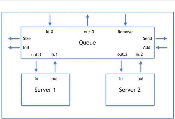
the figure 1.2 presents a system which has the ability to change its struc-ture, by changing its coupled component into a 1-server or 2-server structure. If the server1 in this node is idle, it can be removed and transferred to another node. However, if a 3-server structure is not anticipated and integrated into

sχ, the node cannot have a 3-server structure. In a complex use case where

the combinatorial structure cannot be planned, DSDEVS is not suitable. According to the definition, the set of components is defined, but their state is not. Barros thus defines the new components states after a χ transition to be equal to the same components state before transition (plus time advance) if the component existed or to be the initial state if the component didn’t exist.

Figure 1.2: A DSDEVS exemple: block diagram of a node

1.2.2.2 Parallel Dynamic Structure DEVS

Parallel Dynamic Structure DEVS (DSDE) [Barros 1998] defines a specific component, χ, as for DSDEVS, whose state encodes the structure of the net-work. The current network structure can be obtained at any time from χ state using the structure function γ.

DSDE atomic components syntax defined as PDEVS atomic compo-nents

DSDE coupled components syntax The DSDE component is defined as for DSDEVS:

DSDEN =< XN, YN, χ, Mχ >

However, the model of the executive χ is an extended definition of an atomic model defined as:

Mχ =< Xχ, Sχ, s0,χ, Yχ, γ, Σ∗, δχ, λχ, τχ > where

γ : Sχ → Σ∗ is the structure function

In this definition, χ is the only component allowed to change the network structure. Moreover, the connections between the components of the network are also defined by χ state, i.e. a simple change of connector without affecting the atomic components themselves must be treated as a χ transition.

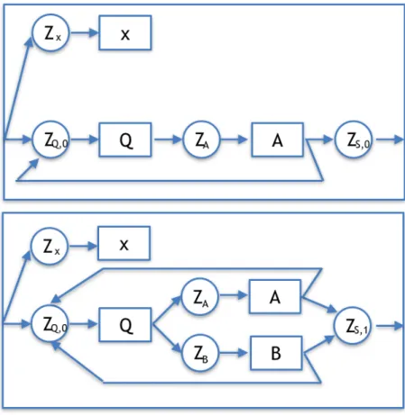
Figure 1.3: A DSDE exemple: one server network change to two sever network

An exemple of a buffered server [Barros 1998] is presented in figure 1.3. It is composed of the buffer Q and the single server A. When the waiting queue is long, it can hire a new server B.

The buffered server is defined by :

S =< XS, YS, χ, Mχ > where

YS = J∗

J = {c0, c1,...,cj,...} is a set of clients

J∗ is a sequence of jobs

Mχ = = (Xχ, s0,χ, Sχ, δχ, τχ) with Xχ = {change} Sχ = {s0,χ, s1,χ} τs0,χ= τs1,χ = ∞ δχ(s0,χ, e, change) = s1,χ δχ(s1,χ, e, change) = s0,χ

γ(s0,χ)=(D0,{Mi,0},{Ii,0},{Zi,0})

γ(s1,χ)=(D1,{Mi,1},{Ii,1},{Zi,1})

where

D0= {Q,A}

D1= {Q,A,B}

MQ,0= MQ,1=(XQ, s0,Q, SQ, YQ, δQ, λQ, τQ)

MA,0= MA,1=(XA, s0,A, SA, YA, δA, λA, τA)

MB,1= (XB, s0,B, SB, YB, δB, λB, τB) IA,0= IA,1=IA={Q} Iχ,0= Iχ,1=Iχ={S } IQ,0= {S, A} IS,0= {A} ZQ,0: XS× XA→ XQ

ZA,0= ZA,1=ZA and ZA: XQ → XA

Zχ,0= Zχ,1=Zχ and Zχ: XS → Xχ

ZS,0: YA → YS

IB,1= {Q} , IS,1= {A, B}, IQ,1= {S, A, B}

ZB: XQ → XB

ZS,1: YA× YB → YS

The network initial structure is presented at the top of figure 1.3 and when the executive receives an order to hire a new server it changes to the state represented in the botton of figure 1.3. The network can return to its initial structure after firing server B.

1.2.2.3 Conclusion on DSDEVS and DSDE

DSDEVS and its parallel version DSDE propose the first approach to dynamic structure systems representation. They describe a model based on different architectural states between which the components can switch.

However, the formalism given to represent these architectural states is either too general or too specific. It can list all the available architectural states by representing them as sets of sets, or provide a specific, limited list of available states. In the second case, the formalism can be adapted to represent a system in which a well-known set of states is reachable. But in the first case, the formalism lacks an expressiveness and relies on the simulation architecture for providing helper functions such as for adding or removing a component.

Moreover, DSDEVS way of taking into account component internal state change is limited. DSDEVS states that, when a new component appears in the simulation, it is automatically in its initial state, while all other components remain in their previous state. However, no traceability is provided to identify which components are new or not.

1.2.3

Dynamic DEVS and its dynamic port extension

The principle of Dynamic DEVS (dynDEVS) as described in [Uhrmacher 2001] is that each atomic component has its own model transitions function ραwhich

controls its own structural transformation. At coupled component level, the equivalent function is the network model transition function ρN. The model

transition functions can pass from one structure to another. However, it does not consider the context management. Uhrmacher later developed ρ−DEVS, a dynDEVS variation supporting dynamic ports.

Under dynamic DEVS, the original definition of DEVS is changed to cap-ture reflectivity by a recursive definition of models. Its transitions may pos-sibly give rise to “new” models. A model changes its structure, i.e., its state space and its behavior pattern.

1.2.3.1 Dynamic DEVS (dynDEVS)

dynDEVS atomic components syntax A dynamic DEVS is a structure:

dynDEV S =df < X, Y, minit, M(minit) > where

X, Y structured sets of inputs and outputs

minit ∈ M(minit) the initial model

M(minit) is the least set having the structure

{< S, sinit, δext, δint, ρα, λ, ta > |

S the set of states sinit ∈ S the initial state δext:Q × X → S the external

transition functions with Q={(s, e) : s ∈ S, 0 ≤ e ≤ ta(s)} δint:S → S the

internal transition function ρα : S → M(minit the model transition function

λ : S → Y the output function ta : S → R+₀ ∪ {∞} the time advance function }

and satisfying the property

∀n ∈ M(minit).∃m ∈ M(minit).n = ρα(sm)withsm ∈ Sm) ∨ n = minit

dynDEVS coupled components syntax Networks (alias coupled mod-els) do not add functionality to atomic models, since each network can be expressed as an atomic model (due to the DEVS closure under coupling prop-erty).

A dynamic network, dynNDEVS, is the structure:

dynN DEV S =df < X, Y, ninit, N (ninit) > where

X, Y structured sets of inputs and outputs

ninit∈ N (ninit) the start configuration

N (ninit) the least set having the structure<

D, ρN, {dynDEV Si}, {Ii}, {Zi,j}, Select >

D the set of component names

ρN :S → N (ninit) the network transition function with S =

×_d∈DL

m∈dynDEV SdS

m

1.2.3.2 ρ-DEVS

This extension [Uhrmacher 2006] introduces dynamic ports and allows for multiple connections. It authorizes the models to enable or disable certain interactions at the same time.

ρ-DEVS atomic components syntax An atomic ρ-DEVS model is the structure:

ρ − DEV S =< minit, M, XSC, YSC, minit >

with minit ∈ M the initial model, XSC, YSC ports to communicate structural

changes, M the least set with the following structure:

< X, Y, S, s0, δint, δext, δcon, ρα, λρ, λ, ta >

λρ : S × XSC → M: model transition

ρ-DEVS coupled components syntax A reflective, higher order network, or coupled components is defined as:

ρ − DEV SN =< ninit, N , XSC, YSC, minit >

N the least set with the following structure < X, Y, C, M C, ρN, ρα > where

C set of components wich are of type ρ-DEVS

M C set of multi-couplings

ρλ : Sn → YSC: structural output function

A multi-coupling mc ∈ M C is defined as a tuple

mc =< {(Csrc.port)|Csrc ∈ C}, {(Ctar.port|Ctar ∈ C}, select >

1.2.3.3 Conclusion on DynDEVS and ρ-DEVS

DynDEVS and its extension deal with the atomic components reconfiguration which was not addressed in DSDE. It adds the atomics the capability to change their inner behavior with no changes on the coupled level. However, despite this interesting additional capability, DynDEVS still lacks details on how the state of the component is handled when facing a reconfiguration.

The ρ-DEVS extension deals with the external interface of atomics when an internal structure change occurs. This aspect is very interesting with regard to the dynamic behavior of components.

1.2.4

Synthesizable DEVS

Synthesizable DEVS (SynDEVS) is proposed by Molter [Molter 2012]. It is a hardware/software co-design flow based on DEVS model of computation. It proposes a co-simulation process with a DEVS-based formalism and dis-tinguish hardware and software partitions during the simulation. It creates a VHDL-based hardware DEVS and a C++-based software DEVS. It considers the development process for a model of computation relying on simulation. However, it focuses neither on hardware nor on software. The definition of the hardware platform relies on a direct DEVS state-machine to Finite State Machine implementation. It considers the actual hardware clock to match the simulation clock.

Moreover, the model structure of SynDEVS is not dynamic. We have been inspired by its design flow approach, but not its formalism.

SynDEVS atomic components syntax SynDEVS atomic component is denoted by a 15-tuple

SynDEV Satomic =< Pin, Pout, X, Y, V, W, vinit, v, S, s0, δint, δext, δcon, λ, τ >

X Y, S, s0, δint, δext, δcon, λ, τ defined as Zeigler’s

V variables

W values for each variable

vinit initial values for each values

v variable assignment functions

SynDEVS coupled components syntax A coupled components, called as parallel components by Gregor Molter:

SynDEV Sparallel =< Pin, Pout, X, Y, M, Cin, Cout, Cinner >

Pin input ports

Pout output ports

X event values for each input port

Y event values for each output port

M inner atomic or parallel components

Cin connections between input ports and inner components

Cout connections between inner components and output ports

1.2.4.1 Conclusion on SynDEVS

SynDEVS deals with hardware/software codesign. It proposes an interesting view of the codesign problem using the DEVS formalism. However, it tries to make the hardware architecture stick very closely to the DEVS state-machine and time representation. In SynDEVS, the hardware clock is the simulation clock. If this aspect brings interesting real-time applications, it restains the applicability and brings lots of constraints which can be avoided when working in, discrete, simulated time.

1.2.5

Reconfigurable DEVS

Reconfigurable DEVS (RecDEVS) [Madlener 2013] considers dynamic hard-ware MoC together with DEVS. RecDEVS proposes a model based on DEVS for final use on reconfigurable hardware like FPGA. In RecDEVS the system executive Cχ is in charge of the structure changes. However RecDEVS takes

into account some hardware specificities from the beginning, like component communication relying on a bus structure with an address notion. This limits the model to an use on the target platform defined by RecDEVS. Thus, there is no separation between PIM and PDM. There are other limits on the meta-model itself, like the fact that a component deletion can only be triggered by the component itself. Eventually, there is no final implementation on FPGA, the workflow only goes to SystemC simulation.

RecDEV S accounts for the various special properties of reconfigurable

hardware architecture, like the bus architecture. Its concept is based on rep-reseting the reconfigurable hardware blocks as DEVS components.

RecDEVS defines an unique identifier ID for each component.

RecDEVS atomic components syntax The difference between a RecDEVS atomic component and a PDEVS component is that the ports and messages are redefined.

CRecDEV S _{=< X}#_{, Y}#_{, S, s}

0, δint, δext, δcon, λ, τ >

S , s0, δint, δext, δcon, λ, τ as PDEVS

X# _{: I × I × Data}

Y# _{: I × I × Data}

I = {C_dID | d ∈ D, ID ∈ N }, a communication between two components is performed by sending a message onto a blobal communication system. Each message consists of a tuple (sender, receiver, data), where sender, receiver ∈

RecDEVS coupled components syntax

NRec =< Xext, Yext, D, Cχ> where

D : Set of all available DEVS components

Cχ : is the network executive which is a DEVS atomic component

RecDEVS dynamic semantics The creation of new RecDEVS compo-nents consists of a fixed sequence of messages as follows:

∗ if the component CID

orig wants to create a new component of type d ∈ D,

it sends a message (CID

orig,Cχ,(new d)) to the network executive.

∗ Cχ receives the message and performs an external transition δext. This

will create a new RecDEVS component Cid

d and add it to the list of

instantiated components

∗ A confirmation message (Cχ, CorigID , (confirm Cdid )) with the address of

the new component is then sent to the originator.

∗ Starting from the reception of the confirmation message, the originator can address the newly created component.

Figure 1.4: A RecDEVS exemple: add a new component

1.2.5.1 Conclusion on RecDEVS

RecDEVS proposes the first simulator aiming at supporting dynamic structure models on partially reconfigurable architectures. Moreover, many interesting notions, such as the identifier adjoined to the component in order to uniquely identify it.

Nevertheless, RecDEVS models have to include low-level, platform-related, description elements. This ties the models deeply with the execution platform,

preventing them from being adapted to other simulators. This goes against the MDA approach in which the models are platform-independent.

Furthermore, the component context aspect is not treated. When dealing with dynamic component, the context is of prominent importance. For exam-ple, we may want to suspend a component at one time and resume it later from the same point. If the component has to be removed meanwhile, this can only be done by supporting context saving and reloading.

1.3

Dynamically

reconfigurable

computing

systems

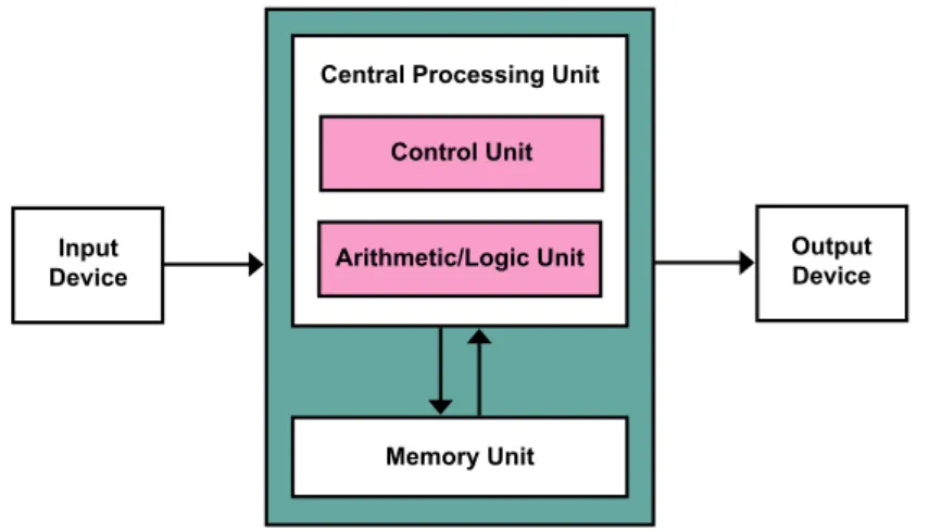
Under earlier Von Neumann architecture by 1950 [Iannucci 1988], as shown in figure 1.5, an electronic digital computer consists in a processing unit, a control unit, a memory, external mass storage and input and output mechanisms. The processing unit is made of an arithmetic and logic unit and processor registers. The control unit contains instruction registers and program counter. The memory stores both data and instructions.

Figure 1.5: Von Neumann Architecture (Image “Von Neumann Architecture”

by Kapooht, available on Wikimedia Commons, CC-BY-SA-3.0) After 60 years of development, the ability of computing using a processing unit arrives at a high level: a system on chip [Xu 2005] has a maximum CPU clock rate up to 3 GHz [Deleganes 2002], compared to the first Intel 4004 at 740 kHz [Aspray 1997]. However, CPU’s are sequential processing devices, even if multi-cores CPUs are developed nowadays, allowing for multiple simul-taneous processings. Compared to a CPU, the parallel nature [Adamski 2005]