HAL Id: tel-03230692
https://tel.archives-ouvertes.fr/tel-03230692
Submitted on 20 May 2021
HAL is a multi-disciplinary open access
archive for the deposit and dissemination of sci-entific research documents, whether they are pub-lished or not. The documents may come from teaching and research institutions in France or abroad, or from public or private research centers.
L’archive ouverte pluridisciplinaire HAL, est destinée au dépôt et à la diffusion de documents scientifiques de niveau recherche, publiés ou non, émanant des établissements d’enseignement et de recherche français ou étrangers, des laboratoires publics ou privés.
centralized and distributed discrete event systems
Hassan Ibrahim
To cite this version:
Hassan Ibrahim. SAT-based diagnosability and predictability analysis in centralized and distributed discrete event systems. Artificial Intelligence [cs.AI]. Université Paris Saclay (COmUE), 2016. English. �NNT : 2016SACLS539�. �tel-03230692�
NNT : 2016SACLS539
Thèse de doctorat
de l'Université Paris-Saclay
préparée à l'Université Paris-Sud
Ecole doctorale n
◦580
Sciences et technologies de l'information et de la communication
(STIC)
Spécialité de doctorat : Informatique
par
M. Hassan Ibrahim
Analyse à base de SAT de la diagnosticabilité et de la
prédictabilité des systèmes à événements discrets centralisés et
distribués
Thèse présentée et soutenue à Orsay, le 16 décembre 2016. Composition du Jury :
M. Stefan Haar Directeur de recherche (Président du jury) INRIA & ENS Cachan
M. Stéphane Lafortune Professeur (Rapporteur) University of Michigan
M. Lakhdar Saïs Professeur (Rapporteur) Université d'Artois
M. Hervé Marchand Chargé de recherche (Examinateur) INRIA
M. Laurent Simon Professeur (co-directeur de thèse) Université de Bordeaux
M. Philippe Dague Professeur (Directeur de thèse) Université Paris-Sud
I want to acknowledge the financial support of this thesis by a scholarship from the Syrian government, in particular from the High Institute of Applied Sciences and Technology (HIAST), and also by the University Paris Sud. I would like to specially thank the responsibles at HIAST for their care of to continue the funding to the maximum possible degree despite the very hard conditions in my beloved Syria.
I would like to thank the reviewers of this thesis, Professors Stéphane Lafortune and Lakhdar Saïs for the valuable time, they have allocated in order to evaluate the quality of this work, despite of their busy schedules. Many thanks also to Professor Stefan Haar and Dr. Hervé Marchand for accepting to be members of my thesis committee.
During this thesis, I had the chance to work with some amazing researchers, from whom I have learned a lot and to whom I would like to acknowledge the results of this thesis. First of all is Professor Philippe Dague, I would like to thank him for his patience, encouragements, guidance and his permanent availability for discussion (even at nights or in the weekends), his passion for science and for work in general is an example that I will never forget. Actually this thesis would not given its fruits without his guidance and his constructive comments during our continuous discussions. I would like to thank also my co-supervisor, Professor Laurent Simon who kindly proposed to supervise this thesis at the beginning and despite of his early move to another university, his comments and feedbacks on my work were always constructive and allowed me to see the work from another perspective to see more and learn more.
I would like to thanks also Alban Grastien and Lina Ye for their interesting discussions and collaboration. Double thanks to Lina for her continuous encouragements and support to keep going on during my hard moments.
I want also to thank all LRI members and especially LaHDAK team members, where I have done this thesis, although my topic was not so compatible with their current research topics but I tried to retain as much as I can from them and their seminars! Thanks also for financing my summer schools and conferences.
Many thanks to my officemates Céline, Camille and Martin for breaking the boredom of the office hours by their friendly conversation, for the knowledge I acquired from them about
France and also for giving me the chance to practice and improve my French with native speakers with very different talking speeds!. I hope that we will keep in touch and that our paths cross again.
Living far from the family in Syria was not so easy, and here is where our friends come to compensate us and to add the flavor of a family to our life. I want to thank from all my heart Wassim and Yara for standing with me and my small family in this last year and especially in these last busy days of my thesis, I wish the best for you and your families!. Thanks also to Haidar, Alessandro for all your support.
I will never forgot to thank my family in Syria, who despite of the hard conditions in Syria did not stop of thinking of us and supporting us in all the ways. My parents, my father-in-law and mother-in-law, my sisters (Maryam and Zeina), my brother (Mohammad) and my cousins (Assil, Awos, Alaa, Rahaf, Ali and Usama), so thank you all again and again! Finally, all my love and thanks to my wife (Hadil) and my son (Jad) for their endless love and support in all my hard days during these thesis, without you I would not ever arrived to this point. You are the hope of my life.
Complex systems are omnipresent in our lives, but subject to failures that it is important to detect or predict. Discrete event system (DES) modeling is a natural way to represent and study such systems formally. Thus a system can be described by a set of states such that its current state is obtained after firing a sequence of events. These events are predefined in a finite set and can be fired spontaneously in the system. Not all these events are observable (measurable) and some of them are considered faulty, thus they model an abnormal change between two system states.
The diagnosis process in DES aims at determining with certainty if the system is currently in a faulty state or in a normal one, i.e., if an abnormal change of a system state has occurred or not. To this end, a system observer has only the sequence of observable events to decide the current status of the system state. However this state might be currently ambiguous (normal or faulty) according to the available observations. Moreover it can be permanently ambiguous! The possibility to disambiguate it using a finite number of observations is called the diagnosability of a faulty event occurrence. The fault is diagnosable if all its occurrences are diagnosable and the system is diagnosable if all its faults are diagnosable. Similarly, the possibility to predict a future occurrence of a fault using its preceding observable events is called the predictability of a faulty event occurrence. Both problems of diagnosability and predictability can be generalized to study the diagnosability or the predictability of a pattern of events, i.e., an extension-closed language represented by a finite state machine.
This thesis considers in its first part the problems of checking event diagnosability, event pre-dictability and pattern diagnosability in centralized and distributed (with observable or unobservable synchronous communication events) discrete event systems, using SAT solvers. Thus we have encoded them as SAT problems, studied incremental SAT variants and provided experimental results that prove the scalability and flexibility of this approach. In the second part, we have introduced the diagnos-ability planning problem. This problem consists in finding a plan of actions (intentional/designful predefined events) that ensures, when applied on a set of potential current system states (called a current belief state), to drive the system in a diagnosable belief state from which it can be left to run freely (without control actions). This problem can arise after an external intervention on the system, like the application of a repair plan after a fault detection.Thus this approach can ensure the possibility to detect the system further faults. We analyzed this problem, proved its PSpace-completeness and proposed three methods to find the intended plan that we compared on a benchmark created for this purpose.
List of figures vii
List of tables ix
1 General Introduction 1
1.1 The Origin of the Story: about Logic, Control, Information and Diagnosability 2
1.2 Contributions . . . 6
1.3 Thesis Organization . . . 7
2 Preliminaries 9 2.1 Introduction to Fault Diagnosis . . . 9
2.2 Modeling Formalism . . . 10
2.2.1 Labeled Transition Systems . . . 11
2.3 Diagnosability . . . 14
2.3.1 General Assumptions . . . 15
2.3.2 Diagnosability Checking in Centralized DES . . . 16
2.3.3 Diagnosability Checking in Distributed DES . . . 19
2.4 SAT Problem . . . 25
2.4.1 SAT Algorithms and Heuristics . . . 28
2.4.2 Succinct Transition Systems . . . 35
2.4.3 SAT-based Diagnosability Encoding . . . 36
3 SAT-Based Diagnosability Analysis in Distributed DES 41 3.1 Motivation/Introduction . . . 41
3.2 Distributed Succinct Transition Systems . . . 43
3.2.1 Modeling . . . 43
3.2.2 Encoding DSLTS Diagnosability as Satisfiability Problem . . . 45
3.2.3 Implementation and Experimental Testing . . . 47
3.3 Diagnosability Checking using Incremental SAT . . . 50
3.3.1 Diagnosability as Incremental Satisfiability . . . 51
3.3.2 Experimental Results . . . 54
3.4 Conclusion . . . 56
4 SAT-Based Predictability Analysis in Centralized and Distributed DES 59 4.1 Motivation/Introduction . . . 59
4.2 Predictability Problem . . . 60
4.2.1 Traditional Predictability Checking in Centralized and Distributed DES 61 4.2.2 SLTS Predictability as Satisfiability . . . 63
4.2.3 DSLTS Predictability as Satisfiability . . . 66
4.2.4 Experimental Results . . . 67
4.3 Predictability Checking Encoding in Incremental SAT . . . 68
4.4 Discussion and Conclusion . . . 71
5 SAT-based Encoding of Pattern Diagnosability in DES 73 5.1 Motivation/Introduction . . . 73
5.2 Definitions . . . 75
5.3 Related Works . . . 76
5.4 SAT Encoding of Pattern Diagnosability in SLTS . . . 78
5.5 SAT Encoding of Pattern Diagnosability in DSLTS . . . 83
5.6 Conclusion . . . 83
6 Diagnosability Planning for Controllable DES 85 6.1 Motivation/Introduction . . . 85
6.2 Diagnosability Planning Problem for Controllable DES . . . 88
6.2.1 Controllable Discrete Event Systems . . . 88
6.2.2 Diagnosability in Controllable DES . . . 89
6.2.3 Planning . . . 91
6.2.4 Problem Definition . . . 91
6.3 Complexity . . . 92
6.4 Solving the Diagnosability Planning Problem . . . 93
6.4.1 Analyzing the Problem . . . 93
6.4.2 Learning and Exploiting Bad and Good pairs . . . 95
6.4.3 General Algorithm . . . 96
6.4.4 Illustrative Example . . . 98
6.6 Related Works . . . 106
6.7 Conclusion and Future Work . . . 107
7 Conclusion 109 7.1 Thesis overview . . . 109 7.1.1 Diagnosability . . . 109 7.1.2 Predictability . . . 110 7.1.3 Pattern Diagnosability . . . 111 7.1.4 Diagnosability Planning . . . 112 7.2 Future Works . . . 112 References 117 Appendix A Synthèse 123
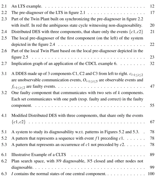
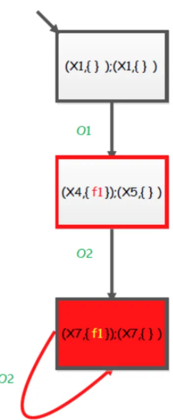
2.1 An LTS example. . . 12 2.2 The pre-diagnoser of the LTS in figure 2.1 . . . 17 2.3 Part of the Twin Plant built on synchronizing the pre-diagnoser in figure 2.2
with itself. In red the ambiguous state cycle witnessing non-diagnosability. 20 2.4 Distributed DES with three components, that share only the events {c1, c2} 21 2.5 The local pre-diagnoser of the first component (on the left) of the system
depicted in the figure 2.4 . . . 22 2.6 Part of the local Twin Plant based on the local pre-diagnoser depicted in the
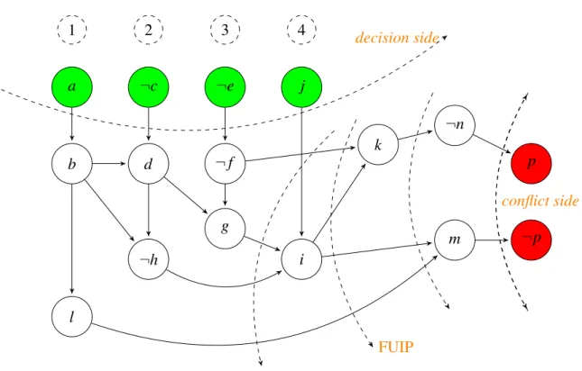
figure 2.5 . . . 23 2.7 Implication graph of an application of the CDCL example 6. . . 32 3.1 A DDES made up of 3 components C1, C2 and C3 from left to right. ci,1≤i≤2
are unobservable communication events, Oi,1≤i≤5 are observable events and
fi,1≤i≤2are faulty events. . . 47
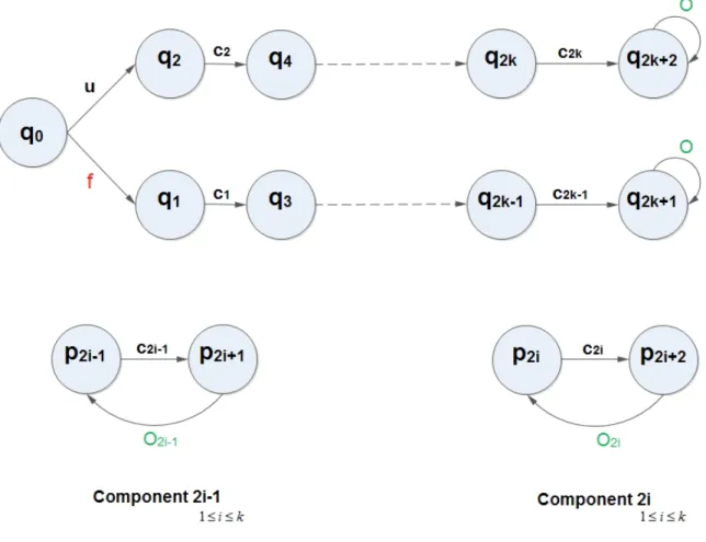
3.2 One faulty component that communicates with two sets of k components. Each set communicates with one path (resp. faulty and correct) in the faulty component. . . 55 4.1 Modified Distributed DES with three components, that share only the events
{c1, c2} . . . 67 5.1 A system to study its diagnosability w.r.t. patterns in Figures 5.2 and 5.3. . 78 5.2 A pattern that represents a sequence with event f 1 preceding c1. . . 78 5.3 A pattern that represents an occurrence of c1 not preceded by c2. . . 78 6.1 Illustrative Example of a CLTS . . . 89 6.2 Plan search space, with N9 diagnosable, N5 closed and other nodes not
diagnosable. . . 99 6.3 I contains the normal states of one central component. . . 100
6.4 Icontains the normal states of two scattered internal components. . . 104 6.5 Changing initial belief state size in a fixed system of (10 × 10) components. 104
3.1 Diagnosability Testing Results on the example of Figure 3.1. . . 49
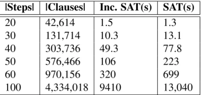
3.2 Results on the faulty component of Figure 3.2. . . 56
3.3 Results on the whole system of Figure 3.2. . . 56
4.1 Diagnosability Testing Results on the example of Figure 4.1. . . 69
4.2 Predictability Testing Results on the example of Figure 4.1. . . 70
6.1 The three methods tested on different grid heights (with width 3) using BFS, where I is made up of the normal states of the central component. . . 101
6.2 The three methods tested on different grid heights (with width 5) using BFS, where I is made up of the normal states of the components at (|lines|/3, 1) and (2|lines|/3, 3). . . 101
6.3 The two learning methods tested on different grid heights (with width 3) using the greedy heuristics, where I is made up of the normal states of the central component. . . 102
6.4 The two learning methods tested on different grid heights (with width 5) using the greedy heuristics, where I is made up of the normal states of the components at (|lines|/3, 1) and (2|lines|/3, 3). . . 102
6.5 The Normal method and the two learning methods with the greedy heuristics tested on a fixed 10 × 10 grid, where I is made up of the normal states of an increasing number of components on the diagonal of the grid (and for the last line all components). . . 103
General Introduction
“If you want new ideas, read old books!"— Ivan Petrovitch Pavlov
This thesis is about diagnosability and predictability analysis in Distributed Discrete Event Systems using a propositional logic approach, in particular using SAT solver. So, what is this? Even if you try to look for the word diagnosability in an Oxford dictionary, you will not get any answer and it may take you, in an any online dictionary, to the word diagnosis, which means “the identification of the nature of an illness or other problem by examination of the symptoms”, which is usually used in a medical context. Translating the word in French will return, if it returns something, the word "diagnosticabilité" not a more meaningful one even for native French speaker!! If you move to predictability maybe you will get more results but most of them will be irrelevant to our predictability meaning here. If you search for diagnosability or predictability analysis in Distributed Discrete Event Systems you will get tens of the scientific articles that we will browse in the next section and chapters and will relate them to our work in this thesis. Finally adding the SAT solver to it in the google search will often give you the work in [Rintanen & Grastien 2007], which is our starting point in this thesis. However, before getting on our work, you may want to see our compilation of some historical points which gives you the intuition or the message of the work from our point of view. This compilation contains mostly historical events taken from Wikipedia pages! connected to show our intuition why the SAT-based approach may work, even if the usage and the formalism used to get the experimental results are not yet discussed. It is only an intuition and you may even re-read this introduction as a conclusion! Last point here, if you are familiar with all the keywords, you may want to proceed directly to the contributions section and come back to this compilation later.
1.1
The Origin of the Story: about Logic, Control,
Infor-mation and Diagnosability
Since the beginnings of humanity on earth, human beings did not stop the interactions with the surrounding nature, firstly, each human being was empowered only by his five senses to do this interaction. He measured the different threats around him to be able to take the decision that keeps him safe to survive. Motivated by his innate curiosity/desire to interact, he developed his tools till creating languages, which allow him to communicate and constructed communities that guaranteed his domination against other species on the planet. After inventing writing, his experiences became more available, endurable (accumulative) and reinforced again his power. Although after the invention of languages humans were crowned on the throne of organisms, however some pioneers from this species continued, and are still continuing, giving the humanity its big cultural strides, through studying the natural phenomena affecting this mankind. They were always guided by their imagination and forte desire to understand and to control this surroundings for the benefits of mankind, especially that they realized how insignificant human beings are, in terms of energetic resources, in comparison to other species, not really recognizing the power of the amazing tool they created, i.e., the languages. For this purpose they have developed different measures continuously to understand this surroundings before controlling it with the less possible effort. Their new ideas started by reading the very old book given by the nature; through it trying then to emulate beings from their surroundings by developing models, lows and rules to describe and simulate these beings and even the natural phenomena.
Hereafter some examples that are related historically to our story are mentioned. Thus, in order to study dynamics of moving objects Isaac Newton invented the laws of physics. Then the laws of thermodynamics were set and the first realization of the so-called system was done by Nicolas Léonard Sadi Carnot in 1824; through organizing some interconnected components such that each component has a functionality that serves to achieve a global mission of the system. Actually it was a body of water vapor that works when heat is applied to it and it was named the working substance in steam engines, thus it can work for a neighbor by pushing it. Rudolf Clausius generalized the picture in 1850 of the working substance by considering the surroundings of the working substance thus it became the system with known limits so we can define its input and output.
In 1854, George Boole introduced Boolean algebra in his book The Laws of Thought which has been fundamental in the development of digital electronics, and is provided in all modern programming languages. It is also used in set theory and statistics. Boolean logic is credited with laying the foundations for the information age.
Actually at that time laws of thermodynamics were not taken directly for granted and prov-ing them was not devoid of adventure and skepticism. Thus solvprov-ing the famous Maxwell’s daemon paradox, that tried to contradict the second law, took many years. This law implies the existence of a quantity called the entropy of a thermodynamic system. Which is used to measure the disorder of a system.
Thus the daemon appeared able to do the job of filtering/classifying gas particles into two classes at free cost. Falsifying this view was in 1929, when Leo Szilard proposed that doing the job by measuring the gas particles cannot be done at free cost which means that the daemon should have negative entropy from the act of acquiring information which would require an expenditure of energy. This negative entropy can be seen as information. In other words, Maxwell’s daemon gets the entropy from the collected information and uses it to decrease the entropy of the “observed” gas. In fact Szilard did not just “save” the second law of thermodynamics but also explained to all humanity how the information can be considered as a form of energy that justifies this kind ability to hold the leadership over this planet!
Later, the work of Szilard was the starting point for Claude Shannon to state the basics of information theory and to Alan Turing to state the computation theory. Thus, Shannon assumed correct computation (encoding, decoding) to get reliable communication and storage over a noisy communication channel, while Turing assumed the correctness of storage and communication to get the computation which is realized using Von Neumann architecture of an electronic digital computer and opened the way for the emergence of computability, functionalism and artificial intelligence.
Algorithmic information theory was introduced in the 1960s by Ray Solomonoff and later was developed independently by Andrey Kolmogorov in 1965 and Gregory Chaitin around 1966 as the subfield of information theory and computer science. It is the information theory of individual objects, using computer science, and concerns itself with the relationship between computation, information, and randomness. The information content or complexity of an object can be measured by the length of its shortest description.
Nowadays humans are controlling systems that they have created everywhere and from all sizes. Thus, the origin of the story is that we want to check if we can control a system at a given price (represented by observations cost) and the cost of resources to do the checking process (represented by the efficiency of our method). In other words, to identify a system situation (or diagnosis). Actually a system is much more than a diagnosis, but diagnosing aims at answering a specific question about the system, it is like projecting all the acquired information about the system on one of two classes. Diagnosability, which as we said above can be seen as the ability to diagnose, is the problem of ensuring that there is at most two classes of diagnoses. It is classifying possibilities into two classes. The ambiguity is always
the third class that raises difficulty and observations are the way to organize the picture for a clearer vision about the system.
Discrete Event System (DES) model is a natural projection of the normal human thinking of the dynamics of a system. Thus we tend to differentiate several stations of a system behavior, let us call them states, and some spontaneously events that take the system’s state to its successor state. In discrete event systems, the output of the diagnosis can be the set of behaviors that explain the observations, where faulty events will be discovered in the results. Diagnosability is the ability to have a precise diagnosis, i.e., given a set of observations paths, have exactly one label of diagnosis, either faulty or correct, consistent with them.
Nowadays systems are omnipresent and they are more and more complex and distributed, the need to control these systems is essential as they are always subject to faults. Thus one wants to know if a system is doing its intended mission (so it is in a normal state otherwise in a faulty one). In order to represent such states in the system, many formalisms can be adopted to model the system like discrete, continuous or hybrid. We adopt here the one which is the closest to the human way of thinking, as we mentioned above, i.e., the discrete one. However, the size of these systems and their distributed nature do not allow them to be fully observable, as such assumption would require very high costs of sensors and measurement process. For this, an abstraction over the system view is applied. However, this lack of information can prevent or complicate diagnosing a fault, i.e., identifying the current system status after having acquired some observation. The problem of the diagnosability of faults means here the ability to detect them after a finite number of observations that proceed their occurrence.
The first introduction to the notion of diagnosability in discrete event systems was by [Sampath et al. 1995]. The authors introduced an approach to test this property by constructing a deterministic diagnoser. However, in the general case, this approach is exponential in the number of states of the system, which makes it impractical.
In order to overcome this limitation the work in [Jiang et al. 2001] introduced the Twin Plantapproach, which uses a special structure called Twin Plant. This approach turns the diagnosability problem into a search for a path with a cycle in a finite automaton, and this reduces its complexity to be polynomial of degree 4 in the number of states (and exponential in the number of faults, but processing each fault separately makes its linear in the number of faults).
Let us mention here that the two previous works were interested in centralized systems with simple faults modeled as distinguished events. The first studies about (surveillance or supervision) patterns were introduced in [Jéron et al. 2006] and [Genc & Lafortune 2006a] which generalize the simple fault event in a centralized DES to handle sequences of events
considered together as a fault, or multiple occurrences of the same fault or of different faults, or more generally any given behavior to be monitored.
The first work that addressed diagnosability analysis in Distributed DES (DDES) was [Pencolé 2004]. A DDES is modeled as a set of communicating Finite State Machines (FSM). Each FSM has its own events set, synchronous communication events being the only ones shared by at least two different FSM. Thus it also depends on the construction of local Twin Plants then synchronizing them incrementally and using some abstraction to avoid constructing the global Twin Plant of the system. The work by [Ye & Dague 2010] has optimized the construction of local Twin Plants. The generalization to patterns in DDES was introduced by [Ye et al. 2010].
After the reduction of diagnosability problem to a path finding problem by [Jiang et al. 2001], it became transferable to a satisfiability problem like it is the case for planning problems [Kautz & Selman 1992]. This was done by [Rintanen & Grastien 2007] which formulated the diagnosability problem (in its Twin Plant version) into a SAT problem, assuming a cen-tralized DES with simple fault events. The authors represented the studied transition system by a succinct representation (cf. section 2.4.2). In fact, the main difficulty in diagnosability algorithms is how to reduce the amount of information that must be acquired to retrieve the diagnosability decision which in turn is related to the difficulty of states number explosion. SAT solvers, which are very powerful tools for checking efficiently the satisfiability of propo-sitional/Boolean logical formulas, are now ubiquitous in artificial intelligence and they can deal with such problems. Such propositional formulas consist of n different Boolean variables participating partially or totally in each of m different clauses, each clause being a disjunction of its participating variables. They help to break the diagnosability question into smaller questions to check if the system description is not violating specific constraints. SAT solvers exploit the statistical approaches and the logical reasoning powers. Their heuristics allow them to compile the tested formula into a simpler description and to introduce randomness in its browsing which can reduce the complexity of deciding if it is satisfiable or not.
Actually the results presented in [Rintanen & Grastien 2007] show a good scalability in comparison with the Twin Plant approaches which the authors said to be impractical for systems with number of states larger than 10000 (actually, the literature contains almost no benchmark or experimental results of the Twin Plant approach and does not propose code availability, so real comparison is difficult). And as we mentioned above this approach considered only centralized DES. This motivated us to consider this approach our starting point, and try to add communication events to consider the distributed DES case and to study the effect of employing incremental SAT mode in both centralized and distributed cases through providing the experimental results of our study, which will be presented in Chapter 3.
From another side, we noticed that many similar problems like predictability analysis which consists in verifying the existence of an observable sequence that reveals with certainty that the fault will occur (see Chapter 4) and pattern diagnosability (see Chapter 5) can be encoded using similar techniques without passing by sophisticated structures used in the literature to deal with such cases.
Our contribution can be informally summarized by saying that we can answer efficiently each of these “ability to know” problems about large systems by “speaking logically” with a SAT Solver, which will intelligently summarize our language into a “small” number of well ordered dependent questions to deduce the answer. This is instead of building a sophisticated structure which requires a larger amount of information to be constructed and then checking a necessary and sufficient condition to decide the problem.
1.2
Contributions
The first part of this thesis is based on an existing approach to check diagnosability in centralized discrete event systems using SAT solvers; this approach is recalled in chapter 2 and our contributions in this part are presented in chapters 3,4,5. Thus, we reviewed the following problems in the literature and provided for each one a propositional logic formalism that is implemented and tested using the SAT solvers technology:
• Diagnosability of simple faulty events in distributed discrete event systems. We extend in chapter 3 the existing formalism in order to consider the synchronous communication events and we show how our encoding is smooth enough such that changes in this encoding are just by adding synchronization formulas without changing the internal encoding of each component. This encoding pushes the synchronization cost to the SAT solver and can consider observable and unobservable communications simultaneously. The flexibility will be exploited for dealing with other similar problems. We show how scalable this approach is through experimental results, which show clearly in particular the efficiency to prove non-diagnosability. However, proving diagnosability in SAT has not the same efficiency, the same concern (SAT vs. UNSAT result) appears in many problems that are reduced to SAT. We propose an approach that mitigates this problem using the incremental mode of SAT solvers, hence we modify the problem encoding to adopt this mode then we test this encoding on an artificial benchmark in centralized and distributed DES and we show its benefits on performance and scalability.
• Predictability of event occurrence in centralized and distributed DES. We exploit in chapter 4 the flexibility of adding and removing constraints in order to model the
predictability problem as a SAT one. This property is stronger than diagnosability and it consists in verifying the existence of a prefix that precedes the event f under consideration such that it reveals with certainty that f will occur each time after it has been seen. We test our encoding and show the scalability of this approach. Then we propose an encoding making use of incremental SAT to exploit the learned constraints about the system behavior, this can help in a more efficient verification which is also automated.
• Pattern Diagnosability. We propose in chapter 5 an encoding for the problem of pattern diagnosability, which generalizes the diagnosability of a specific event to consider any formal extension-closed rational language of events. Actually we have implemented this part but not yet tested it.
The second part of this thesis is presented in Chapter 6 where we introduce the problem of diagnosability planning in controllable DES. This problem, not yet considered in the literature to the best of our knowledge, consists in finding a plan of actions (taken from given elementary control actions) that, when applied on a given belief state (a set of potential current states), drives the system into a diagnosable belief state in order to be able to let the system run from its new initial belief state freely, i.e., without any control but however with guaranteed diagnosability. This problem may appear after a repair plan which leaves the system in a set of potential states from where the diagnosability of the system has not been yet ensured. It is also interesting, when possible, to replace the active diagnosability by diagnosability planning as a monitoring approach in order to reduce the diagnosis interactions with a running system that may add potential cost and affect the availability of the awaited services from the system, e.g., in monitoring power networks. In this part our contributions are the following:
• Formalizing the diagnosability planning problem. • Analyzing and proving its complexity class.
• Proposing three methods to solve the problem efficiently.
• Implementing and testing these methods on an artificial benchmark that we created for this purpose.
1.3
Thesis Organization
This thesis consists of seven chapters; five main chapters in addition to this introduction chapter and the conclusion and future works chapter. The second chapter reviews the state
of the art mainly about the diagnosability problem in centralized and distributed DES, in particular it reviews the Labeled Transition System formalism used in the literature to study this problem showing the main approaches. Then we recall in some detail the starting point of this thesis which is the work of [Rintanen & Grastien 2007] which introduced the succinct transition systems that we used to encode the different cases studied here. The third chapter presents our first contribution which is the extension of the existing approach to consider communication events in the formalism then to adopt the encoding to be processed by an incremental SAT solver. In the fourth chapter we consider the predictability property and we encode it using the succinct transition systems into a SAT problem in both centralized and distributed structures. The fifth chapter is devoted to present our encoding of the pattern diagnosability problem as a SAT problem. The second part of the thesis is presented in the sixth chapter where we introduce the problem of diagnosability planning in controllable DES, this part is not strictly disjoint from the first part as we will use the Twin Plant structure recalled in chapter 2, however we do not use SAT technology in this part even if it is mentioned in the future work sections in the last chapter where we conclude.
Preliminaries
In this chapter we provide the preliminaries required to follow this thesis, that will be cited in the next chapters whenever needed. It contains the formal definitions for the system model that we adapted in our study, like labeled transitions systems in centralized and distributed versions. We recall also the diagnosability problem definition and review how it is addressed in the literature. The basics to understand Satisfiability problem will follow, then we recall the succinct transitions systems in their centralized version and show how they have been used to encode the diagnosability problem in SAT.
2.1
Introduction to Fault Diagnosis
Diagnosis task is mainly using the available observations to explain the difference between the expected behavior of a system and its real behavior which may contain some faults. Systems are around us everywhere in our life, and as they are always subject to faults, therefore fault diagnosis is an important domain that will be always needed to ensure the safe availability of these systems. Examples of diagnosis application can be found in domains such as transportation from vehicles to spacecrafts, infrastructure like water or power networks and in software and hardware testing in addition to many complex systems. This wide appearance motivated from many years a lot of works to study the automatic approaches to do system fault diagnosis [Bavishi & Chong 1994, Sampath et al. 1996, Sampath et al. 1998, Ushio et al. 1998, Debouk et al. 2000, Grastien et al. 2007]. They all try to deal with the main problem which is the compromise between the number of possible diagnoses to the faulty system and the number of observations which must be given to make the decision. The diagnosis problem is NP-hard and one always needs to cope with an explosion in the number of system model states.
In general faults can be classified according to their lasting time in transient, intermittent or permanent faults. A transient fault occurs accidentally usually after an external interference then disappears before detecting it leaving some effects on the system. An intermittent fault leaves the system in an alternating state between normal and abnormal; like a malfunctioning device in a situation that does not respect its operating conditions of temperature and voltage, or because of the interaction among not fully compatible devices. A permanent fault leaves the system in a faulty state until its reparation, this can be an effect of a physical damage that needs to be repaired. We are interested in this thesis in permanent faults.
In model based diagnosis, faults could be modeled by states, so the diagnosis question would be whether the system is currently, using the current observation, in a faulty or a normal state. They can be also modeled as faulty events assigned to some transitions of the system, and so the diagnosis question will be whether a faulty event occurred or not, after regarding the set of available observation coming from the system’s sensors. We are interested here in faults represented as faulty events.
The problem is that the diagnosis question must be answered precisely in order to take the appropriate action; for example in case of an affirmative answer, i.e. the fault has oc-curred, one can proceed to isolate the faulty components of the system and later repair them. However, in a definitive negative answer the system is ensured to be running correctly which is the normal purpose of a system. Otherwise, one can wait to acquire more observation if the current state is undetermined, i.e., can be reached with either a faulty behavior or a normal one. However, the diagnosis decision maybe always uncertain, and thus running a diagnosis algorithm may not be accurate. For example, two sets of observations provided by different sets of sensors or at different times may lead to different diagnoses, one faulty and the other normal. This uncertainty raises the problem of diagnosability which is an essential property to be ensured while designing the system model. It simply means the ability to get a precise diagnosis. After that, the model based diagnosis will be used in applications to explain any anomaly, with a guarantee of correctness and precision at least for each anticipated fault in the model.
2.2
Modeling Formalism
First of all, we define what is a system, following the IEEE definition “A system is a combination of components that act together to perform a function not possible with any of the individual parts”. To this end the system is represented by a model, which represents the evolution from one state to a successive one through transitions. A state of the system, or
simply a state, describes the system current status, usually using a vector of state variables which are identified to this purpose. Transitions can be synchronized to a time clock and so each state will represent the system status at a specific time-step, or can be assigned to some event, from an asynchronous set of events, in this case a state will hold the required information to represent the last event’s effects which led to the current state. Transitions can also be modeled using a combination of the event and a time tag to represent the event’s time occurrence or some temporal condition related to this event.
In this thesis we use timeless model, so transitions are assigned only to a set of events which are asynchronous in the centralized case and will have some synchronous events that connect the different components in the distributed case.
In the fault diagnosis domain, three types of systems are considered, the continuous systems, the discrete systems and the hybrid systems. We are interested in discrete systems and in particular in Discrete Event Systems (DES) which are discrete-states, events-driven systems, that is, their states evolution depends entirely on the occurrence of asynchronous discrete events over time in the centralized case and on both synchronous and asynchronous discrete events in the distributed case.
The discretization of states and events is widely used to represent dynamics of a system in an abstract manner due to its direct reflection to the human way of thinking and visualizing. Even continuous systems can be qualitatively abstracted to discrete ones in some ways. Actually this discretization facilitates modeling, analyzing and designing systems in order to do further steps like synthesizing, controlling these systems and evaluating their performance or optimizing them. The most popular computation models used to study the diagnosis problem are the Petri Nets (PN) and the Finite State Machines (FSM), or more generally the Labeled Transition Systems (LTS), which we will adopt as an input model due to its simplicity, However this model will be translated into a succinct representation in order to use SAT Solvers in this thesis.
2.2.1
Labeled Transition Systems
Labeled transition systems are formal models that are widely used to design and to represent real systems through abstracting their behaviors by sequences of transitions; thus they reflect how the system progresses between its different states respecting the design rules. In other words, the behavior of the system is represented by the language generated by the finite state machine. In their graphical representation, usually we denote states by circles and transitions by arrows that connect these circles, events appear as labels over the arrows.
x1 x5 x2 x4 x3 x6 x7 f1 O1 c1 O1 c1 c1 c1 O2 c1 Fig. 2.1 An LTS example.
Example 1 (LTS example). The figure 2.1 represents an LTS system with 7 states, two main types of events: observable like {O1, O2} and unobservable like { f 1, c1} with f 1 a faulty event.
We adopt the labeled transition system as a modeling formalism and we define it here following [Sampath et al. 1995] .
Definition 1. @ A Labeled Transition System (LTS) is a tuple T = ⟨Q, Σ, δ , q0⟩ where: • Q is a finite set of states,
• Σ = Σo∪ Σu∪ Σf is a finite set of events,
• δ ⊆ Q × Σ × Q is the transition relation, • q0is the initial state.
with Σothe set of observable correct events, Σuthe set of unobservable correct events and Σf
the set of unobservable faulty events.
Demanding only one initial state q0is actually not a limitation: if there are several ones, one creates a unique new one and connects it by unobservable transitions to each of the previous ones. δ is trivially extended recursively to words in Σ⋆(the Kleene closure of Σ): δ ⊆ Q × Σ⋆× Q. Formally speaking, we denote by L(T ) the prefix-closed language generated by T , which is a subset of Σ⋆. Thus the system behaviors are represented by the set of words
of this language: L(T ) = {σ ∈ Σ⋆|∃qs∈ Q, (q0, σ , qs) ∈ δ }. We call a path ρsin the system,
any alternating sequence of states and events obtained from the initial state q0and ending with a state qs ∈ Q: ρs = q0 e1 → q1 e2 → · · · en → qs, with e1, . . . , en∈ Σ, q0, q1, . . . , qs∈ Q and
∀i ∈ {0, . . . , n − 1}, (qi, ei+1, qi+1) ∈ δ . We denote the length of a path ρs by |ρs|.
A path ρs defines a (part of) system behavior σs, that can be viewed as a possible run and is
called a trajectory of the system: σsis the abstraction of ρson its sequence of events between
the initial state q0and the last state qs, i.e., σs= e1. . . en∈ Σ⋆is the trajectory corresponding
to ρs . Clearly this abstraction is not one-to-one in a non-deterministic system, thus the same
sequence of events, or trajectory, can be assigned, in general, to more than one path. We call the projection of such a sequence on its observable events an observable sequence σo; it can
be obtained by applying the instance Poof the general projection operator, Pa(.) : Σ⋆→ Σ⋆a,
where Σais the intended subset of events to retain, i.e., on which to abstract. Pa(.) is defined
as follows: Pa(.) =
Pa(ε) = ε, ε is the empty event, Pa(e) = ε, if e /∈ Σa,
Pa(e) = e, if e ∈ Σa,
Pa(eσ ) = Pa(e)Pa(σ ), where e ∈ Σ and σ ∈ Σ⋆.
(2.2.1)
As a result, the set of possible system runs that can be related back to an observable sequence σo is defined like this: Po−1(σo) = {σ ∈ Σ⋆|Po(σ ) = σo}. One can notice that
differentiating from each other the sets of faulty and non-faulty paths in a system, based on its observations, is highly related to the sizes of these sets of possible trajectories, which in their turn depend on the degree of non-determinism in the system that can be reduced each time a new observations arrives.
We denote the post-language of L(T ) after the trajectory σ by L(T )/σ , it represents the possible continuation of σ in the transition system T . L(T )/σ = {t ∈ Σ⋆|σ .t ∈ L(T )}.
Operations on Labeled Transition Systems
In order to study the diagnosability problem we will need to define formally some operations on the LTS, like synchronizing two LTS and performing a delay closure on a LTS.
Definition 2. (Synchronization) Given two LTS, T1= ⟨Q1, Σ1, δ1, q01⟩ and T2= ⟨Q2, Σ2, δ2, q02⟩,
we define their synchronization T1||ΣsT2, on a predefined synchronization set of events
Σs⊆ Σ1∩ Σ2, as a new LTS T1||ΣsT2= ⟨Q1× Q2, Σ1∪ Σ2, δ1||2, (q 0
1, q02)⟩ with δ1||2defined as
follows:
• ((q1, q2), σ , (q′1, q2)) ∈ δ1||2if σ ∈ Σ1\ Σsand (q1, σ , q′1) ∈ δ1.
• ((q1, q2), σ , (q1, q′2)) ∈ δ1||2if σ ∈ Σ2\ Σsand (q2, σ , q′2) ∈ δ2.
If we restrict the transition relation δ1||2 only to the first item, i.e., we accept only the synchronization set of events Σs in the result, then the operation is called a product. This
simply can happen when we synchronize two copies of the same system on their common vocabulary.
Definition 3. (Delay Closure) Given an LTS T = ⟨Q, Σ, δ , q0⟩, its delay closure with respect
to Σd, where Σd⊆ Σ, is ∁Σd(T ) = (Qd, Σd, δd, q0), where:
• (q, σ , q′) ∈ δdif σ ∈ Σd and ∃s ∈ (Σ\Σd)∗, (q, sσ , q′) ∈ δ .
• Qd= {q0} ∪ {q ∈ Q | ∃q′∈ Qd, ∃σ ∈ Σd, (q′, σ , q) ∈ δd}.
Thus, this operation eliminates transitions labeled by events not in Σd and is identical to
the classical silent transitions elimination in asynchronous automata.
2.3
Diagnosability
Diagnosability of the considered systems is a property defined to verify the possibility to distinguish any possible faulty behavior in the system from any other behavior without this fault (i.e., correct or with a different fault) within a finite time after the occurrence of the fault. A fault is diagnosable if it can be surely identified from the partial observation available in a finite delay after its occurrence. The first introduction to the notion of diagnosability was by [Sampath et al. 1995]. The authors studied diagnosability of LTS, which is defined in definition 1. They formally defined diagnosability like the following:
Definition 4. (Diagnosability) A fault f is diagnosable in a system T iff (if and only if)
∃k ∈ N, ∀sf ∈ L(T ), ∀t ∈ L(T )/sf, |t| ≥ k ⇒ ∀p ∈ L(T ), (Po(p) = Po(sf.t) ⇒ f ∈ p.
In this formula, sf denotes any word in Σ⋆f. The above definition states that for each trajectory sf ending with fault f in T , for each t that is an extension of sf in T with enough events, every trajectory p in T that is equivalent to sf.t in terms of observation should contain in it f .
In other words, the fault f is non-diagnosable iff it exists a pair of observation-equivalent infinite trajectories, one with f and the other without f . We call such a pair a critical pair. The absence of such a pair will provide information about fault signature. Finding such a pair will help in positioning the sensors to manage the observations requirements in order to increase diagnosability and ensure robust fault detection and identification.
2.3.1
General Assumptions
Following other studies about diagnosability we adopt the following set of assumptions to be hold in all this thesis.
Assumption 1. (Liveness) The language L(T ) of the trajectories of the studied transition system is live.
This means that for any state, there is at least one transition issued from this state. This assumption ensures that the post-language of L(T ) after any trajectory is never empty, so contains arbitrarily long sequences.
Assumption 2. (Convergence) The language L(T ) of the trajectories of the studied transition system is convergent.
This means that there is no cycle made up only of unobservable events. As studying diagnosability relies on the observations, so accepting infinite behaviors of the system without getting any observation makes the study meaningless.
A system T is said to be diagnosable iff any fault f ∈ Σf is diagnosable in T . In order
to avoid exponential complexity in the number of faults processed during diagnosability analysis, only one fault at a time is considered to check its diagnosability.
Assumption 3. (Fault uniqueness) There exists only one fault event f (Σf = { f }), without
restriction on the number of its occurrences.
This is actually not a restriction. It just means that each fault will be processed separately and successively for checking its diagnosability. During this process, other faults are con-sidered as unobservable correct events, allowing to get linear complexity in the number of faults.
This assumption is actually not necessary if one is interested only in detecting without ambiguity in finite time after its occurrence any fault that happened. But in general, the purpose of this detection is to trigger repair or reconfiguration actions because the fault is assumed to be still present, i.e., to be permanent. We will see later that diagnosability can be extended from the detection of simple events to the detection of complex surveillance patterns, and that it is easy to model intermittent faults with such patterns.
Other assumptions about system and fault modeling will be added when needed in the other chapters.
Next we review the main works done to check diagnosability in centralized and distributed DES. Other works can be seen as variations or optimization on these works and we will mention them in the next chapters in their appropriate places in this thesis.
2.3.2
Diagnosability Checking in Centralized DES
The main difficulty in diagnosability checking algorithms is related to the states number explosion since [Sampath et al. 1995] introduced an approach to test the diagnosability property by constructing a deterministic diagnoser (hence the potential exponential number of states), starting from a non-deterministic pre-diagnoser, and searching for a critical pair of paths, i.e., two arbitrarily long paths which are equivalent from an observation point of view and only one of them contains the fault. The existence of a critical pair witnesses the non-diagnosability while its absence proves the diagnosability of the studied fault. In the following, we recall the definition of these two structures and how such a critical pair can be found.
The pre-diagnoser is a structure that can be obtained by abstracting a system by its observations, while keeping in its states the trace of the fault occurrence. Formally it is defined like the following:
Definition 5. (Pre-Diagnoser) The pre-diagnoser of the system T = ⟨Q, Σ, δ , q0⟩ is an observable LTS, denoted by D = (QD, ΣD, δD, q0D), where:
• QD⊆ Q × 2Σf is the set of states (q, ℓ) with q ∈ Q and l ⊆ Σf that are reachable by δD
from q0D(see below);
• ΣD= Σois the set of observable events;
• δD⊆ QD× ΣD× QDis the set of transitions defined by: δD= {((q, ℓ), e, (q′, ℓ′))
∈ QD× ΣD× QD|∃ a path ρ = (q u1 −→ q1... um −→ qm−→ qe ′) in T , with uk∈ Σu∪ Σf, ∀k ∈ {1, ..., m}, e ∈ Σoand ℓ′= ℓ ∪ ({u1, . . . , um} ∩ Σf);
• q0D= (q0, /0) is the initial state.
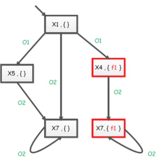
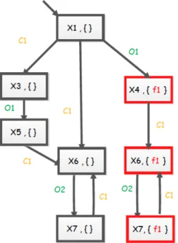
In the pre-diagnoser, we only keep the observable events and attach the fault information to each retained state as a fault label. Precisely, for a unique fault event f , if f has occurred from the initial state up to a given state, then the fault label for this state is { f }. Otherwise, it is empty. And as we consider only permanent faults, all reachable states from a state with a fault label { f } will hold the same label. Figure 2.2 shows the pre-diagnoser of the system in Figure 2.1.
Fig. 2.2 The pre-diagnoser of the LTS in figure 2.1
After having built the pre-diagnoser, the deterministic diagnoser can be obtained by determinizing this structure, which consists in gathering all states that are reachable from a state by the same observable event in one state, while keeping the fault information in each state of the grouped state. We define the deterministic diagnoser as follows:
Definition 6. (Deterministic Diagnoser) Let T = ⟨Q, Σ, δ , q0⟩ be an LTS and D = (QD, ΣD,
δD, q0D) its pre-diagnoser, we denote its deterministic diagnoser by Dd= (QDd, ΣDd, δDd, q 0 Dd),
where:
• QDd ⊆ 2
QDis the set of states that are reachable by δ
Dd from q 0
Dd (see below);
• ΣDd = ΣD= Σois the set of observable events;
• δDd : QDd× ΣDd → QDd is the transition function defined by:
δDd(qd, σ ) = S
qD∈qd∧(qD,σ ,q′D)∈δD{q ′ D};
• q0D
d = q 0
D= (q0, /0) is the initial state.
Since each state in this deterministic diagnoser is an aggregation of states from the states of the pre-diagnoser, which in their turn hold a unique fault label { f } or empty, then a state q1∈ QDd could hold different fault labels. Actually we have, in a general abstraction, three
possible cases:
• F-certain state: in which all grouped (pre-diagnoser) states are with a fault label { f }. This means it can be reached only by passing by a fault occurrence.
• N-certain state: where all grouped (pre-diagnoser) states are with an empty fault label. This means it cannot be reached by passing by a fault occurrence.
• F-uncertain state: where only a sub-part of the grouped (pre-diagnoser) states has the fault label { f } while the other part has the empty fault label.
We recall that a critical pair consists of two infinite paths (in the meaning of cycle), only one of them has the faulty event and they are equivalent in terms of observation. We call a cycle in Dd, an F-undetermined cycle iff:
• all its states are F-uncertain states;
• it has a corresponding cycle in the pre-diagnoser made up of only states with fault label { f };
• it has a corresponding cycle in the pre-diagnoser made up of only states with fault label empty.
In order to search for a critical pair of trajectories in the deterministic diagnoser structure, we can restrict the search for a cycle which is F-undetermined since the determinism of the structure ensures the synchronization of the observations.
It is worth to notice that not each cycle of F-uncertain states in this structure is surely an F-undetermined cycle, while the second and third conditions together imply the first one.
However, in the general case, this approach is exponential in the number of states of the system, which makes it impractical for large systems. A polynomial algorithm to check diagnosability is proposed in [Jiang et al. 2001, Yoo & Lafortune 2002]. The authors introduced a new structure which is called Twin Plant. In order to build this structure we start from the pre-diagnoser for a given system, then we synchronize the pre-diagnoser with itself based on the observable events, i.e., each observable event should be synchronized, to obtain all pairs of trajectories issued from the initial state with the same observations.
Definition 7. The Twin Plant of the system T is the observable LTS T P = D ∥Σo D, where Dis the pre-diagnoser of T .
As we said before, a synchronization process between two copies of the system on its set of events, is equal to a product operation. Each state of the Twin Plant is a pair of pre-diagnoser states that provide two possible diagnoses with the same observations. Given a Twin Plant state, if the fault f is contained in exactly one of the two associated pre-diagnoser states, which means that the occurrence of f is not certain up to this Twin Plant state with the same observations, it is called an ambiguous state with respect to f . An ambiguous state cycle is a cycle containing only ambiguous states. We define a critical path as a path in the Twin Plant issued from the initial state and made up of a prefix followed by an ambiguous state cycle. It corresponds exactly to a critical pair. So, after that, we verify the diagnosability by searching for such a critical path.
Lemma 1 ([Jiang et al. 2001, Yoo & Lafortune 2002]). A system is non-diagnosable iff its Twin Plant contains a critical path.
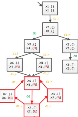
This result is illustrated on the figure 2.3 where the presence of the critical path ((x1, {}); (x1, {}))−→ ((x4, { f 1}); (x5, {}))O1 −→ ((x7, { f 1}); (x7, {}))O2 −→ ((x7, { f 1}); (x7, {})) inO2 the Twin Plant of the LTS example of the figure 2.1 proves that this system is not diag-nosable.
2.3.3
Diagnosability Checking in Distributed DES
A distributed Discrete Event System, or DDES, is a system with a set of communicating components, each one of them can be represented as an LTS and they share a set of events among each other. Under the assumption of a global observation of the system, the author of [Pencolé 2004] proposed the first approach to check diagnosability of Distributed Discrete Event Systems. He considered communications to be correct events that are not observable. Formally speaking, he defined a DDES as a set of m local models Ti, 1 ≤ i ≤ m, sharing
synchronous communication events, where a local model is defined as follows:
Definition 8. A local Labeled Transition System (lLTS) is a tuple Ti= ⟨Qi, Σi, δi, q0i⟩
where:
• Qiis a finite set of states,
• Σi= Σio∪ Σiu∪ Σif∪ Σic is a finite set of events occurring in Ti,
Fig. 2.3 Part of the Twin Plant built on synchronizing the pre-diagnoser in figure 2.2 with itself. In red the ambiguous state cycle witnessing non-diagnosability.
• q0i is the initial state.
with Σio a finite set of observable correct local events, Σiu a finite set of unobservable
correct local events, Σif a finite set of unobservable faulty local events and Σic a finite set
of communication events, the only ones to be shared by at least another local model of a neighboring component of Ti.
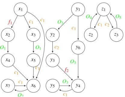
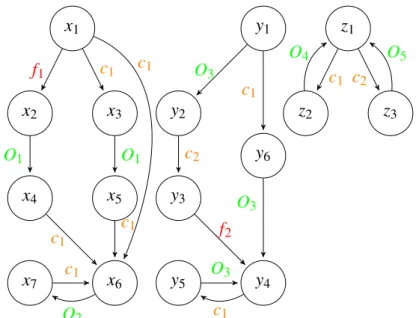
Figure 2.4 depicts a system with three components, that share only the communication events {c1, c2}.
Assumption 5. (Global observation) The system is globally observed.
This means that the observations in the system are globally ordered among the different components of a distributed system.
Assumption 6. (Synchronous communication) The communication events between the different components are synchronous.
x1 x5 x2 x4 x3 x6 x7 y1 y2 y3 y4 y5 y6 z1 z2 z3 f1 O1 c1 O1 c1 c1 c1 O2 c1 O 3 c2 f2 c1 O3 O3 c1 c1 c2 O4 O5
Fig. 2.4 Distributed DES with three components, that share only the events {c1, c2}
Assumption 7. (Communication correctness) The communication events between the different components are correct.
Notice that assuming communication events correct is not a restriction but a matter of modeling: if some communication event may be faulty, then the communication channel involved has just to be modeled as a new component by itself, containing at least one faulty local event.
Under the above assumptions, the problem of diagnosability in DDES is the one defined following the definition 4. Thus, it is to verify if the studied faults are diagnosable in the global system model (or a sub-part of it), which is the product of the local models synchronized on the communication events and on which delay closure with respect to these communication events is then applied: T =∁Σc(||ΣcTi), where Σc= ∪iΣic and Σo= ∪iΣio,
Σu= ∪iΣiu, Σf = ∪iΣif. But one wants this verification to be achieved incrementally, starting
at the level of the components without prior building of the global model.
The author of [Pencolé 2004] introduced an incremental diagnosability test which avoids building the Twin Plant for the whole global system if not needed. For this one starts by building a local Twin Plant for the faulty component to test the existence of a local critical path. If such a path does not exist, we know the system is diagnosable. But, if such a path exists, one should build local Twin Checkers of the neighboring components, i.e., those components which share communication events with the faulty one. The local Twin Checker is a structure similar to the local Twin Plant, i.e., where each path in it represents a pair of behaviors with the same observations, except that there is no fault information in it since it
is constructed from non-faulty components. After constructing local Twin Checkers, one tries to solve the ambiguity resulting from the existence of a critical path in the local Twin Plant, by synchronizing this local Twin Plant with the local Twin Checker of one neighbor on their communication events. In other words, one is trying to distinguish the faulty path from the correct one by exploiting the observable events in the neighboring components. Thus, the occurrences of observable events that are consistent with the occurrences of the communication events could solve the ambiguity. The process is repeated until the diagnosability is answered, which necessarily happens in the worst case when the whole system is visited. Another important contribution in this work was to delete the unambiguous parts after each synchronization on the communication events, in order to reduce the amount of information transferred to the next check (if needed).
The figure 2.5 depicts the local pre-diagnoser of the first component (on the left) of the system depicted in the figure 2.4 and the figure 2.6 part of its local Twin Plant. This one displays a local critical path, proving that the fault f1is not locally diagnosable in the first
component.
Fig. 2.5 The local pre-diagnoser of the first component (on the left) of the system depicted in the figure 2.4
The sizes of the considered parts of each local Twin Plant (or Twin Checker), also called local verifier, is reduced in the work of [Schumann & Pencolé 2007], where the authors describe the diagnosability problem as a distributed search problem. Thus, the global behavior is determined based on the local Twin Plants without computing any part of the
Fig. 2.6 Part of the local Twin Plant based on the local pre-diagnoser depicted in the figure 2.5
global Twin Plant. They propagate the fault information from the faulty component to other components by passing through a computable set of possibly non-diagnosable states in the different local Twin Plants of the different components depending on the connectivity between them and the faulty component. As a result, every state that is not possibly non-diagnosable is certainly non-diagnosable and so is deleted from the local Twin Plant, which leads to a reduced local Twin Plant. After that, the diagnosability of a fault is decided based on the set of distributed Twin Plants. Thus the fault is diagnosable iff none of the reduced Twin Plants contains an observable possibly non-diagnosable cycle (OPNC). A reduced Twin Plant is firstly obtained from the Twin Plant of each component in the system, then reduced Twin Plants are pairwise incrementally synchronized in order to remove remaining OPNCs to prove the diagnosability if possible, otherwise the approach gives a synthetic view of the non-diagnosability by returning all indistinguishable behaviors in the system. Thus one can deduce from the non-diagnosable states all possible critical pairs in the system. This approach is also adaptable to the available resources, thus it can stop when it runs out of memory and returns the current set of Twin Plants with OPNCs which contains all possible reasons for a potential non-diagnosability and which tells also that any set of the original components of the system which participated in any of the current reduced Twin Plants is not sufficient to diagnose the fault.
The work by [Ye & Dague 2010] has optimized the construction of local Twin Plants, by exploiting the fact that one distinguishes two behaviors (faulty and normal) and one synchronizes at two levels (observations first and communications later). The authors improved the construction of the Twin Plants proposed by [Pencolé 2004] by exploiting the different origin of the communication events (left and right copies) at the observation synchronization level to assign them directly to the two behaviors studied (left copy to the faulty behavior and right copy to the normal one). This helped in deleting the redundant information, then in abstracting the amount of information to be transferred later to next steps if the diagnosability is not answered.
Online/Offline Diagnosability Checking and Complexity
As we said before, the main problem while verifying diagnosability is to deal with states number explosion. This verification is usually done in an offline mode, in that the Twin Plant is first constructed, then a critical path is searched in it. Some recent approaches are proposed using Petri nets [Liu et al. 2014] to do the verification on-the-fly while construct-ing the Twin Plant and later by buildconstruct-ing a hybrid diagnoser for verifyconstruct-ing diagnosability [Boussif et al. 2015] by combining enumerative and symbolic representations, passing by a symbolic observer graph [Haddad et al. 2004], in order to build a deterministic diagnoser where on-the-fly technique can be used to reduce the required time and memory resources in diagnosability verification. However, approaches that use the non-deterministic pre-diagnoser are still, to the best of our knowledge, to be done in an offline mode.
The complexity of the Twin Plant approach proposed in [Jiang et al. 2001] is polynomial of the 4th degree, in terms of states number. This can be seen easily, from its definition, where the number of states in the pre-diagnoser is bounded by (|Q| × 2|Σf|), then the number
of states in the Twin Plant is bounded by (|Q|2× 22|Σf|), which allows a search space of
(|Q|4× 24|Σf|× |Σ
o|). Thus finding a critical path in the Twin Plant is polynomial in the
number of system states and exponential in the number of faults. Therefore, we consider one fault at a time while checking diagnosability of the system, as we mentioned in assumption 3. The worst case while checking diagnosability appears when the studied system is actually diagnosable. It implies proving the nonexistence of a counter-example witnessing non-diagnosability, i.e., all possibilities need to be tested as for proving the nonexistence of a plan in a planning problem, and usually in this case some approximations are used to avoid exploring all the search space, but we do not consider such approximations in this thesis. Testing diagnosability was proved to be NLOGSPACE-hard for enumerative representations, and PSPACE-hard for succinct (symbolic) representations [Rintanen 2007]. However, when using succinct representations, one can apply more abstract reasoning through using modern
efficient tools like BDD (Binary Decision Diagram) tools or model checkers and SAT solvers. Actually the reduction of the diagnosability problem to a path finding problem by [Jiang et al. 2001] made the problem transferable to a satisfiability problem like what is done in planning problems [Kautz & Selman 1992]. The authors in [Rintanen & Grastien 2007] formulated the diagnosability problem (in its Twin Plant version) into a SAT problem assuming a centralized DES with simple fault events. The work in this thesis can be considered as extensions and improvements over what they have done. We will review succinct transition systems used by their work in subsection 2.4.2.
2.4
SAT Problem
The satisfiability problem, or simply SAT problem, is a central theoretical problem in com-puter science, actually it is the canonical NP-problem [Cook 1971] in this field, It consists in answering the following question: given Boolean variables and a conjunction of a set of clausesfrom these variables, which forms a propositional formula in the so called Conjunc-tive Normal Form, denoted by CNF, is there a possible assignment of all these variables (or some of them), such that the logical formula takes the value True for this assignment.
Let us first define some of the terms in the last sentence. First, a Boolean variable, also called a propositional variable, is a symbol of 0-ary predicate which takes its values in the set {True, False} or simply {1, 0} of logical truth values. An assignment (resp. partial assignment) is a valuation of the variables (resp. of some of them). An assignment satisfying the given formula is called a model for this formula. A formula that owns a model is said to be satisfiable. A formula is built over a set of propositional variables by using the following logical operators or connectives:
• the binary conjunction operator AND, denoted by ∧, • the binary disjunction operator OR, denoted by ∨, • the unary negation operator, denoted by ¬,
• the binary implication operator, denoted by →, • the binary equivalence operator, denoted by ↔.
Actually, the operators above are not independent and we can restrict these operators to, e.g., only the disjunction and the negation operators, the other connectives being easily expressible