A ROBUST AND AUTOMATED FE-BASED METHOD FOR FIXTURELESS DIMENSIONAL METROLOGY OF NON-RIGID PARTS USING AN IMPROVED NUMERICAL INSPECTION FIXTURE
V. Sabri*a, S. Sattarpanahb, S.A. Tahana, J.C. Cuillièreb, V. Françoisb, X.T. Phama
ABSTRACT
Dimensional inspection is an important element in the quality control of mechanical parts that have deviations from their nominal (CAD) model resulting from the manufacturing process. The focus of this research is on the profile inspection of non-rigid parts which are broadly used in the aeronautic and automotive industries. In a free-state condition, due to residual stress and gravity loads, a non-rigid part can have a different shape compared with its assembled condition. To overcome this issue, specific inspection fixtures are usually allocated in industry to compensate for the displacement of such parts in order to simulate the use state and accomplish dimensional inspections. These dedicated fixtures, their installation, and the inspection process consume a large amount of time and cost. Therefore, our principal objective has been to develop an inspection plan for eliminating the need for specialized fixtures by digitizing the displaced part’s surface using a contactless (optical) measuring device and comparing the acquired point cloud with the CAD model to identify deviations. In our previous work, we developed an approach to numerically inspect the profile of a non-rigid part using a non-rigid registration method and finite element analysis. To do so, a simulated displacement was performed using an improved definition of boundary conditions for simulating unfixed parts. In this paper, we will improve on the method and save time by increasing the accuracy of displacement boundary conditions and using automatic node insertion and finite element analysis. The repeatability and robustness of the approach will be also studied and its metrological performance will be analyzed. We will apply the improved method on two industrial non-rigid parts with free-form surfaces simulated with different types of displacement, defect, and measurement noise (for evaluation of robustness).
Keywords: quality control, geometric / dimensional inspection, geometric dimensioning and Tolerancing (GD&T), profile tolerance, registration, non-rigid / flexible / deformable / compliant part, assembly conditions, dimensional metrology.
* Corresponding Author
a. Products, Processes, and Systems Engineering Laboratory (P2SEL), Department of Mechanical Engineering, Ecole de Technologie Superieure (ÉTS), Montreal, QC, Canada
b. Équipe de Recherche en Intégration Cao-Calcul (ERICCA), Department of Mechanical Engineering, Université du Québec à Trois-Rivières, Trois-Rivières, QC, Canada
POSTPRINT VERSION. The final version is published here :
Sabri, V., Sattarpanah, S., Tahan, S., Cuillière, J. C., François, V., & Pham, X. (2017). A robust and automated FE-based method for fixtureless dimensional metrology of non-rigid parts using an improved numerical inspection fixture. In International Journal of Advanced Manufacturing Technology (Vol. 92, pp. 2411-2423): Springer Nature.
1 INTRODUCTION
Dimensional inspection plays a significant role in the quality control of mechanical parts since it usually consumes a large portion of production lead time. By means of Geometric Dimensioning and Tolerancing (GD&T), geometric specifications and product design are specified with respect to functionality. To verify if the specifications defined at the design phase are respected, the GD&T inspection procedure is applied. Using a reliable, efficient, and automated inspection process will result in decreased product life cycle time and improved industrial competition [1]. The dimensional inspection, in the case of rigid parts, has significantly improved and the developed methods are generally applied within the industry [2], whereas the dimensional inspection of non-rigid parts with free-form surfaces is still an ongoing and challenging field of research.
In mechanical engineering applications, surfaces are allocated a profile tolerance to control manufacturing variations [2]. A surface profile should be controlled based on the norms established by the ASME Y14.5-2009 standards (section 8) [3]. According to these standards (or ISO 1101:2004, ISO-GPS standards [4]), unless otherwise specified, all tolerances should be applied in a free-state condition. Exemptions are agreed to this rule for non-rigid parts that may deform significantly from their defined tolerances due to their weight (gravity) or the release of residual stresses resulting from manufacturing processes [3, 5].
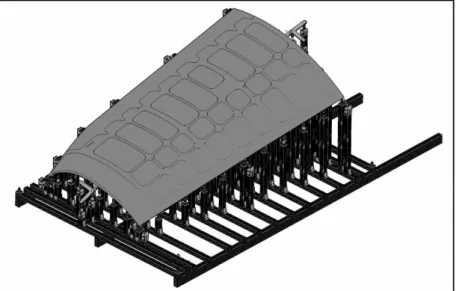
To overcome the above-mentioned issue, specialized inspection fixtures with complex installations are usually used within the industry to compensate for the displacements in order to simulate the use state and perform dimensional inspections of non-rigid parts. These dedicated fixtures are costly, heavy, and complex (Figure 1). The installation and inspection processes are extremely time-consuming which reduces competitiveness. The mentioned standards also agree with the application of reasonable load (not exceeding the load expected under normal assembly conditions) to displace non-rigid parts to conform to the defined tolerances. The solution is to develop an inspection technique for eliminating the need for specialized fixtures by digitizing the displaced part’s surface using a contactless (such as optical) measuring device and comparing the obtained point cloud with the nominal model to identify deviations.
Figure 1: A costly, heavy, and complex fixture dedicatedly installed for the dimensional metrology of a non-rigid plate mounted on it, Bombardier Aerospace Inc.
To compare the digitized data (point cloud) with the nominal (CAD) model, it is essential to dispose these two data sets in a joint coordinate system. This procedure is termed registration. In modern technologies, registration is mathematically defined using the translation and the rotation of the Design Coordinate System (DCS) with respect to the
Measurement Coordinate System (MCS). In application, registration can be done in two stages: searching for the correspondence relationship between nominal and digitized surfaces; and, defining an optimum transformation matrix between the DCS and MCS. The rigid registration methods are applied only for rigid parts. In flexible parts, the registration problem requires the application of a non-rigid registration method on top of finding a rigid mapping. The difference between rigid and non-rigid registrations is that a non-rigid registration can align two different shapes (for example, a line with a curve) [6, 7]. Numerous methods have been developed for rigid and non-rigid registration such as the Iterative Closest Point (ICP) algorithm [8] and its variants for rigid registration; the Multi-Dimensional Scaling (MDS) method [9], and the Coherent Point Drift (CPD) algorithm [10] for non-rigid registration applied in medical imaging, animation, etc. However, for the registration of a non-rigid mechanical part, the situation is different due to the result of its compliance behavior.
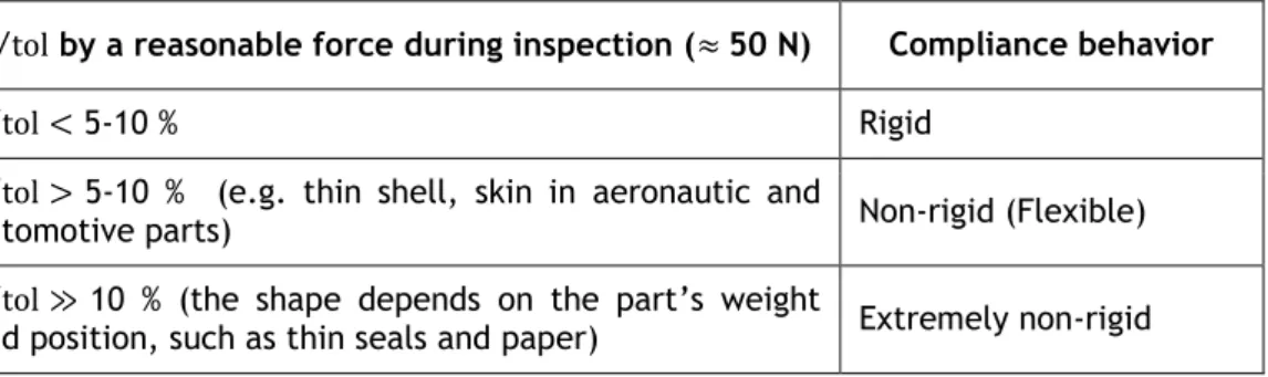
Compliance behavior of a compliant (flexible) part is a vital issue to study while specifying tolerances and assessing the geometric and dimensional specifications for the part. This element is a relative concept based on the relation between an imposed force and its resulting displacement [11]. Based on the displacements of parts stemming from a reasonable force (50 N) during dimensional inspection, the parts are considered rigid / non-rigid (flexible) / extremely non-non-rigid (see Table 1). For quantifying the flexibility of a mechanical part from an industrial point of view, another method was proposed by Aidibe and Tahan [12]. Their quantifying method is based on the ratio between the maximum displacement (δ) induced by a certain force and the profile tolerance of the non-rigid part. Our research is on typical non-rigid mechanical parts used in the aeronautic and automotive industries.
Table 1: The ratio 𝛅 𝐭𝐨𝐥⁄ in each zone induced by a force during inspection and their
compliance behaviour
δ tol⁄ by a reasonable force during inspection (≈ 50 N) Compliance behavior
δ tol⁄ < 5-10 % Rigid
δ tol⁄ > 5-10 % (e.g. thin shell, skin in aeronautic and
automotive parts) Non-rigid (Flexible)
δ tol⁄ ≫ 10 % (the shape depends on the part’s weight
and position, such as thin seals and paper) Extremely non-rigid
A review of previous research on the fixtureless dimensional inspection of non-rigid parts is discussed in the next section. In this paper, we present an improved version of a previous approach proposed by our team [13]. This new approach is improved mainly with respect to the displacement boundary conditions used in FE-based non-rigid registration and to the automation of node insertion. This improved inspection method is described in section 3. Case studies along with an evaluation of repeatability and an analysis of metrological performance are presented in section 4. The paper ends with a conclusion.
2 REVIEW OF PREVIOUS RESEARCH
Ascione and Polini [14] discussed the dimensional inspection of non-rigid parts with free-form surface using inspection fixtures combined with Coordinate Measuring Machine (CMM). Abenhaim et al. [11] presented a review of previous research on the fixtureless inspection of non-rigid parts and proposed a classification of the specification methods used for the GD&T of non-rigid parts under the ASME and ISO standards. In the following, we will introduce the primary methods, based on a simulated displacement approach, developed for the dimensional inspection of non-rigid parts without the use of inspection fixtures.
A first attempt at the fixtureless inspection of non-rigid parts was undertaken in 2006 by Weckenmann et al. [15, 16]. The authors proposed the virtual distortion compensation method in which they virtually displaced the distorted manufactured part into the nominal model by displacing the point cloud acquired using a contactless measuring device. A triangle surface mesh was generated from the point cloud and transformed into a finite element analysable (FEA) model. Afterwards, the positioning process was simulated using information about the assembly features’ deviation from the actual (measured) to the ideal (nominal) position. In this method, human intervention is needed to recognize the correlation between some determined points and assembly conditions in order to define the boundary conditions of the FEA problem. Hence, boundary conditions can be improved to simulate a real model of the positioning system. Moreover, converting the digitized data (point cloud) into a FE model is a time-consuming process loaded with uncertainties. One year later in 2007, Weckenmann et al. [17] improved on the shortcomings of their previous work by displacing a CAD model towards the measurement data in the virtual reverse deformation method. They enforced the boundary conditions on the CAD model using the known position of the fixation points on the scanned part. Thus, a pre-processing of the digitized data is not required. Through this method, they decreased inspection time and achieved more precise results. The FE simulation of the displacement boundary conditions on the geometrically ideal CAD model is evidently more accurate. Nevertheless, this method still required human intervention to find the corresponding relationship between the CAD model and the measurement data. Furthermore, the modelling of the boundary conditions in the FE dataset needs to be improved to simulate the unfixed part.
Analogous to the virtual reverse deformation method, Jaramillo et al. [18, 19] presented an approach which requires less calculation power, using the Radial Basis Functions (RBFs) to minimize the finite element mesh density required to correctly predict part behavior. Recently in [20], they improved upon their method by performing the registration of flexible part using only partial views from areas that needed inspected. They applied an interpolation technique based on RBFs to estimate positions of the missing fixation points since the partially digitized data may not contain all of them.
Gentilini and Shimada [21] proposed an approach for the shape inspection of a flexible assembly part by virtually mounting it into the assembly. First, the dense measured mesh is smoothed and reduced to become suitable for FEA. Material properties, if not available, are defined by a calibration process. Then, specific displacement boundary conditions are defined and applied for the FE simulation of the assembly process. Once FEA is performed, quality inspection of the simulated post-assembly shape is done using visualization tools. Moreover, the virtual post-assembly shape is compared with the real one for an evaluation of method accuracy. This method can predict the final assembled shape of a flexible part, but it has the drawbacks mentioned in the virtual distortion compensation method. The polygonal mesh data suffers from uncertainties, noise and a high quantity of polygons, therefore it needs post-processing steps, smoothing and decimation.
In 2012, Radvar-Esfahlan and Tahan [22] presented the Generalized Numerical Inspection Fixture (GNIF) method based on the distance preserving property of non-rigid parts: the shortest path (geodesic distance) between any two points on the surfaces does not change during an isometric displacement in spite of large displacement. By taking advantage of this property, the algorithm looks for some correspondence between the scanned part and the CAD model. The authors used the Multidimensional Scaling (MDS) approach in order to find a correspondence between two metric spaces (CAD model and scanned part). Then, finite element non-rigid registration (FENR) was executed knowing some boundary conditions. The dimensional deviations between the displaced CAD model and the digitized data can be identified after the FENR. Correspondence search is completely automatic. The GNIF dealt with a very general case of non-rigid inspection. The authors used the borders for FENR in the absence of assembly conditions. This situation may not conform to assembly conditions and real use state. Boundary conditions for the simulated displacements can be improved
based on assembly conditions. The authors in [23] robustified the GNIF method by filtering out points that cause incoherent geodesic distances. The improved method is able to handle parts with missing digitized data sets.
In contrast to the aforementioned methods, Abenhaim et al. [24] proposed the Iterative Displacement Inspection (IDI) method that is not based on the FEA module. This method iteratively displaces the meshed CAD model until it matches to the digitized data. The IDI algorithm is based on optimal step non-rigid ICP algorithms [25] which combine rigid and non-rigid registration methods. Also, an identification method was developed for distinguishing surface deviations from the part’s displacement. This method displaces the CAD mesh regarding its smoothness and prevents covering surface defects and measurement noise during the mapping process. Aidibe et al. [26] improved the identification module of the IDI algorithm by proposing the application of a maximum-normed residual test to automatically set the identification threshold. However, the IDI method has certain drawbacks. Due to a lack of FE analysis, the method depends on identifying some flexibility parameters which are reliant on thickness. In addition, they use the same number of nodes in the two data sets.
Aidibe and Tahan [12] presented an approach that integrates the curvature properties of manufactured parts with the extreme value statistic test as an identification method for comparing two data sets and to recognize profile deviation. This approach was tested on simulated typical industrial sheet metal with satisfactory results in terms of error percentage in defect areas and in the estimated peak profile deviation. As the fundamental of the algorithm is based on the Gaussian curvature comparison, application of the method is limited to relatively-flexible parts where small displacements are predictable. The authors in [27] proposed the IDB-ACPD method for optimization of the CPD algorithm in order to adapt it to the relatively-flexible parts problem, introducing two criteria: the stretch criterion between the nominal model and the aligned one; and the Euclidian distance criterion between the aligned nominal model and the scanned part.
Abenhaim et al. [28] introduced a method that registers the point cloud to the nominal model using information recuperated from the FE model of the CAD model. This is done by embedding a FE-based transformation model into a boundary displacement constrained optimization. This optimization problem tries to minimize a distance-based similarity criterion between points in unconstrained areas whereas this criterion between points in constrained areas is kept in a specified contact distance, and simultaneously, the restraining forces are limited. The latter allows for the inspection of non-rigid parts for which their functional requirements require limiting the restraining forces imposed during assembly. In addition, the point cloud does not need to be pre-processed into a FE model. Also, there is no need for manual identification of fixation positions in the point cloud. Furthermore, as long as the point cloud includes the restraining areas, a partial view of the part can be enough for the method.
An automatic fixtureless inspection approach based on filtering corresponding sample points was presented in [29], wherein corresponding sample points that are in defect areas are automatically filtered out, based on curvature and von Mises stress criteria. This tends to a more accurate inspection of non-rigid parts.
Recently in [30], an approach was proposed to evaluate shape deviations of flexible parts, using optical scanners, in a given measuring configuration for which the setup is known (whatever configuration, independent from the assembly conditions). The CAD model was displaced by the FE simulation of the part’s displacement due to its own gravity considering the known configuration used for the measurement. Having applied to a simple part, the form deviations were recognized by subtracting the simulated geometrical displacements to the measured geometrical displacements. They used the known configuration for the part’s optical measurement based on which the displacement vector for the FE simulation at each
node of the CAD mesh was calculated using the intersection of a cylindrical neighborhood of its normal vector and the point cloud.
3 PROPOSED APPROACH
Searching for correspondence between two data sets, as a primary step, seems to be the best idea in registration problems, according to the literature. As mentioned in the previous section, the GNIF method based on the isometric displacement [22] has some advantages that encourage us to use it to search for corresponding points between two data sets. In our previous work [13], we developed an approach to numerically inspect the profile of a non-rigid part using a non-non-rigid registration method and finite element analysis. To do so, a simulated displacement was performed using an improved definition of displacement boundary conditions for simulating unfixed parts. The developed method was implemented on two industrial non-rigid parts with free-form surfaces simulated with different types of displacement, defect, and measurement noise (for one case). In the current paper, we will improve our method and save the time using the automatic node insertion and finite element analysis. Also, repeatability and robustness of the improved approach will be studied for all the cases. We will apply the improved method on two industrial non-rigid parts; one from the previous work (case B) and a new one (case C). In addition, for repeatability and robustness evaluation, Gaussian measurement noise will be introduced three times to each case (24 times for 8 cases). Therefore, the improved method will be studied on a total of 32 cases.
The Generalized MDS method of non-rigid registration, applied in the GNIF approach, represents the corresponding points on the data sets based on the barycentric coordinate system [22]. To use these points for future purposes, their barycentric coordinates have to be converted into Cartesian coordinates. Using Equations 1 and 2 in [13], the Cartesian coordinates of the corresponding points in each data set can be calculated.
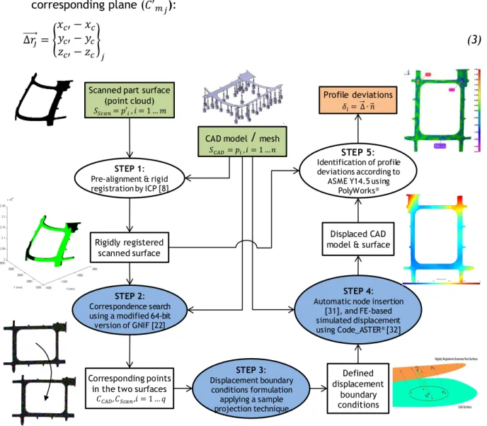
Figure 2 schematically shows the different steps of our approach. First, we displace the scanned part surface (𝑆𝑆𝑐𝑎𝑛 = 𝑝′𝑖 , 𝑖 = 1, … , 𝑚) close enough to the CAD surface (𝑆𝐶𝐴𝐷= 𝑝𝑖 , 𝑖 = 1, … , 𝑛) (pre-alignment) to achieve a satisfactory result for rigid registration using ICP [8]. Then, the pre-aligned surface is rigidly registered to the CAD surface (2D triangle mesh) by using the ICP algorithm. The next step is to apply the modified 64-bit version of the GNIF method to find a set of correspondent pairs between the two surfaces (Equation 1). We have modified the GNIF code, in MATLAB®, and converted the 32-bit version into a 64-bit version to achieve the capability of dealing with high density data sets. In the 32-bit version, the GNIF code can be only applied on meshes with less than 10,000 nodes; whereas using the modified 64-bit version, we can search for correspondence, and consequently apply the proposed method, on any case study with an enormous number of nodes.
𝐶𝐶𝐴𝐷 = {𝑝𝑖|𝑖 = 1, … , 𝑞} 𝐶𝑆𝑐𝑎𝑛= {𝑝′𝑖|𝑖 = 1, … , 𝑞}, 𝑞 ≪ 𝑚, 𝑛 (1) To define a set of displacement boundary conditions for simulating the displacement from the CAD model to the rigidly registered scanned part surface, the constrained areas on the CAD model, such as fixation positions (e.g. hole) or contact surfaces (e.g. target datums) according to ASME Y14.5, are first recognized [21]. Then, the corresponding points (with the Cartesian coordinates) inside each constrained area (with the index of 𝑗), and consequently their correspondents in the scanned data, are identified among all the correspondents obtained by the GNIF method:
𝐵𝑗= {𝑝𝑖 ∈ 𝐶𝐶𝐴𝐷|𝑖 = 1, … , 𝑠𝑗≪ 𝑞}, 𝐵′𝑗= {𝑝𝑖′ ∈ 𝐶𝑆𝑐𝑎𝑛|𝑖 = 1, … , 𝑠𝑗≪ 𝑞} (2) Next, for each area and its corresponding area on the scanned surface, we define a centre of mass by fitting a plane through the identified corresponding points (𝐵𝑗, 𝐵′𝑗). To register each pair of the identified correspondents in the two data sets by simulated displacement using finite element analysis, the displacement boundary conditions should be defined by local translation law [21]:
the centre of mass (𝐶𝑚𝑗) is translated to the corresponding centre of mass on the corresponding plane (𝐶′𝑚𝑗): ∆𝑟𝑗 ⃗⃗⃗⃗⃗ = { 𝑥𝑐′− 𝑥𝑐 𝑦𝑐′− 𝑦𝑐 𝑧𝑐′− 𝑧𝑐 } 𝑗 (3)
Scanned part surface (point cloud)
𝑆𝑆𝑐𝑎𝑛= 𝑝′𝑖 , 𝑖 = 1 … 𝑚
CAD model
/
mesh𝑆𝐶𝐴𝐷= 𝑝𝑖 ,𝑖 = 1 …𝑛
Rigidly registered scanned surface
STEP 2:
Correspondence search using a modified 64-bit version of GNIF [22]
STEP 1:
Pre-alignment & rigid registration by ICP [8]
Corresponding points in the two surfaces
STEP 3: Displacement boundary conditions formulation applying a sample projection technique Defined displacement boundary conditions STEP 4:
Automatic node insertion [31], and FE-based simulated displacement using Code_ASTER®[32]
Displaced CAD model & surface
STEP 5:
Identification of profile deviations according to
ASME Y14.5 using PolyWorks®
Profile deviations 𝑖= ∆ 𝑛
𝐶𝐶𝐴𝐷,𝐶𝑆𝑐𝑎𝑛,𝑖 = 1 … 𝑞
Figure 2: Flowchart of the proposed approach
In the previous paper [13], the displacement vectors were calculated based on the difference between the coordinate of each sample point (centre of mass) on the CAD model and its corresponding sample point on the scanned model. However, the generated sample points for CAD and scanned models based on the presented method are not necessarily located on the pertinent CAD or scanned mesh; this is a source of error in finite element calculation. In the current paper, to increase accuracy of the FE calculation and consequently the non-rigid inspection result, the generated centres of mass are projected individually on their related CAD or scanned models. To this end, each generated sample point is moved along its normal direction respect to the mesh surface to coincide with the related mesh triangulation. Then, the displacement vectors are calculated accordingly based on the difference between the coordinate of each projected sample point on the CAD model and its corresponding projected sample point on the scanned part. Therefore using the sample projection technique, the accuracy of the method is improved in step 3.
Having defined the displacement boundary conditions, the finite element analysis can be performed between the two data sets based on the simulated displacement approach to distinguish between displacements and deviations. The goal is to find the maximum profile deviation on each defect comparing the scan data and the displaced CAD model ( 𝑚𝑎𝑥 in Figure 3). To this aim, the determined centres of mass are inserted into the CAD mesh, and then the CAD model is displaced towards the scanned surface applying the defined
displacement boundary conditions to the inserted centres of mass. In our previous work [13], this node insertion process was performed manually. In the present paper, the nodes (projected centres of mass instead of original ones) are inserted into the CAD mesh automatically using a classical Delaunay point insertion method [31]. Then, each displacement vector is calculated as explained before in the step 3 of the algorithm. Applying FE analysis, the CAD model is deformed towards the scanned model by applying the displacement vectors as the displacement boundary conditions on the projected and inserted sample points on the CAD model. The FEA is performed by applying a new and open source method [32]. In other words, the step 4 of the algorithm is also improved, and we save time and cost.
We have successfully implemented the methodology using several tools. Mesh generation, mesh transformations, and FEA have been done using the research platform developed by our research team [32]. This platform is based on C++ code, on Open CASCADE® libraries and on Code_Aster® as FEA solver. Typically, noise generation and point projection as well as FEA takes almost 1 minute on a computer with Intel® Core™ i7 at 3.60 GHz processor in 31.3 GB RAM.
Finally, the profile deviations ( 𝑖) are identified based on the shortest 3D distance between each point of the scanned data and the displaced CAD surface, as recommended by ASME Y14.5-2009 [3], using PolyWorks® Software. Then on each defect, the maximum profile deviation ( 𝑚𝑎𝑥) is estimated. CAD Model Displaced CAD Model Scanned Part Defect on the Sanned Part Displacement Vectors
Figure 3: Simulated displacement, identification of profile deviations ( ) and estimation of maximum profile deviation ( ) on a defect
4 CASE STUDIES, REPEATABILITY EVALUATION, AND METROLOGICAL PERFORMANCE ANALYSIS
We evaluate our proposed approach on two industrial non-rigid part models (case A and case B) typical in aerospace industries. Parts are illustrated in Figure 4. For each model, different virtual parts with different (but known) displacements and deviations (e.g. bumps) are simulated, and their point clouds are extracted. To simulate the parts, we apply two types of displacement: torsional (typical of displacement due to residual stresses) or, flexural (typical of displacement due to gravity). Two types of defect area (small or big) were simulated with different amplitudes (1, 1.5, 2, or 3 mm) on each model (A and B): ASF, AST, ABF, ABT, BSF, BST, BBF, BBT (Case A or B, S: small defects, B: big defect, F: flexural displacement, T: torsional displacement). There is one defect in the cases with big area defects, and there are three or four defects with different amplitudes in the cases with small area defects. The meshing in all the cases is triangular surface mesh with 5mm size. The number of nodes in the CAD model in case B is 9816, and in case A is 29776. Thus, a correspondence search in case C became possible with the modified 64-bit version of the GNIF code in MATLAB®.
Case B Case A
Figure 4: Non-rigid parts mounted on conformation's jigs, Bombardier Aerospace Inc.; dimensions (mm) of case A: 1750 × 1430, and case B: 1153.4 × 38.6; the material is
aluminium alloy 7050-T7451.
The automatic node insertion technique and FE solver in the step 4 makes us able to evaluate repeatability and study robustness of the approach. Gaussian measurement noise 𝑁(0, 𝜎𝑛𝑜𝑖𝑠𝑒) is introduced three times on each of the above-mentioned simulated cases (24 times for 8 cases) where 𝜎𝑛𝑜𝑖𝑠𝑒 = 0.01, 0.02, 0.03 𝑚𝑚 that is a typical value of the measurement noise for a non-contact scanning device. The noises are generated as random numbers from the normal distribution with mean and standard deviation parameters. These random numbers are added to the nodes coordinate of the scanned mesh in the normal direction respect to the mesh surface. Therefore, the proposed approach is totally applied on 32 simulated case studies: 8 original (noise-free) cases, and 24 cases with noise.
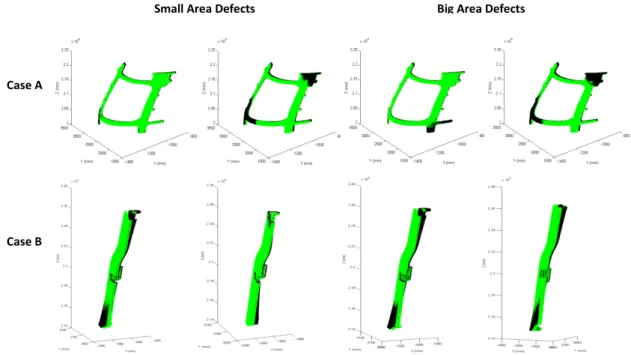
In each case, the pre-alignment and the rigid registration using the ICP algorithm are performed first. Figure 5 shows the simulated parts after this step. Using the modified 64-bit version of the GNIF method, the correspondents between the CAD surface and the rigidly registered surface are identified (Figure 6). To compare the capability of corresponding search between the 32b and the 64b versions of the GNIF algorithm, the calculation time for each original case, on a computer with Intel® Core™ i7-3770 at 3.40 GHz processor in 16.0 GB RAM, is mentioned in Table 2. The number of correspondence sample points is 1000 in the cases B and 2000 in the cases A. There is an insignificant time difference between the 32b and the 64b versions in the case B which is the smaller case (9816 nodes in the CAD model). The main difference is in the case A (29776 nodes in the CAD model) where the 32b version of the GNIF algorithm is inapplicable for the calculation.
Case B
Small Area Defects Big Area Defects
Case A
Figure 5: Simulated parts with different (but known) displacements and deviations, after pre-alignment and ICP rigid registration (step 1)
Case A Case B
CAD model
Scanned Part
Figure 6: Correspondence search by the modified GNIF (step 2) – Examples: ABF and BST Table 2: Capability and calculation time of corresponding search compared between the
32b and the 64b versions of the GNIF algorithm
Cases Calculation time (minutes) 32b GNIF 64b GNIF ASF Inapplicable 126 AST Inapplicable 156 ABF Inapplicable 98 ABT Inapplicable 96 BSF 17 20 BST 23 20 BBF 16 17 BBT 26 19
Knowing the constrained areas and the corresponding points, the displacement boundary conditions are formulated taking advantage of the sample projection technique as described earlier. The projected centres of mass are inserted into the CAD mesh using the automatic node insertion method [31]. Having defined the displacement boundary conditions, using the recently developed FE-based platform [32], the CAD mesh is modified and displaced to the rigidly registered scanned surface (for registration purpose) applying the linear elastic FEA method (Figure 7).
Case A Case B
Figure 7: FE-based simulated displacement using Code ASTER® [32] (step 4) – Examples: ABF and BST
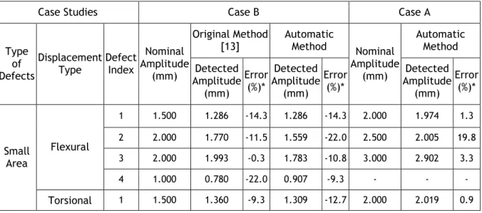
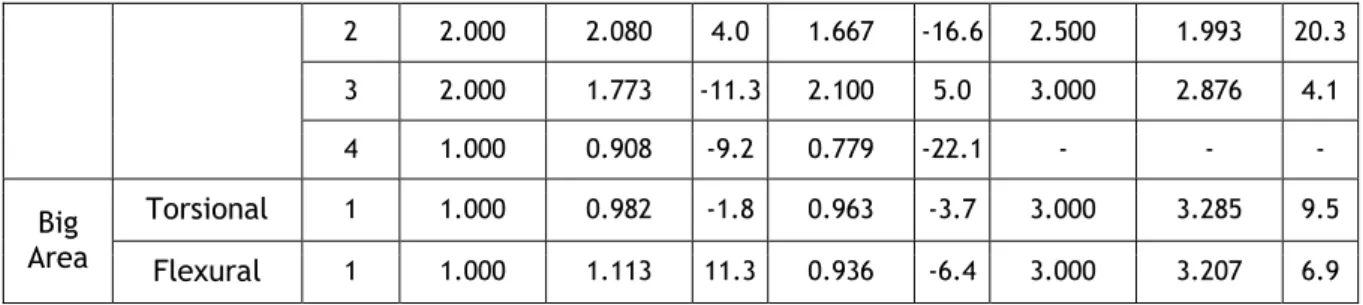
Comparing the displaced CAD surface and the rigidly registered scanned surface, the known deviations are recognized, using PolyWorks®. Table 3 summarizes the amplitude results by the automatic method in each defect compared between the nominal amplitude and the detected (estimated) amplitude in the original noise-free cases A and B. These values, as well as defect positions and areas, are illustrated in Figure 8 (Case A) and Figure 9 (Case B) using the inspection color maps in PolyWorks®. There is a comparison between the results of the original and the automatic method in the noise-free case B in Table 3 as well. For repeatibility evaluation, Table 4 is dedicated to the results of defect’s amplitude in the cases A and B with added noise for repeatability evaluation. The maximum displacement in all of the cases is around 10 mm.
Table 3: Results of defect amplitudes in cases A and B (noise-free), and a comparison between the original and the automatic method in case B
Case Studies Case B Case A
Type of Defects Displacement Type Defect Index Nominal Amplitude (mm) Original Method
[13] Automatic Method Nominal Amplitude (mm) Automatic Method Detected Amplitude (mm) Error (%)* Detected Amplitude (mm) Error (%)* Detected Amplitude (mm) Error (%)* Small Area Flexural 1 1.500 1.286 -14.3 1.286 -14.3 2.000 1.974 1.3 2 2.000 1.770 -11.5 1.559 -22.0 2.500 2.005 19.8 3 2.000 1.993 -0.3 1.783 -10.8 3.000 2.902 3.3 4 1.000 0.780 -22.0 0.907 -9.3 - - - Torsional 1 1.500 1.360 -9.3 1.309 -12.7 2.000 2.019 0.9
2 2.000 2.080 4.0 1.667 -16.6 2.500 1.993 20.3 3 2.000 1.773 -11.3 2.100 5.0 3.000 2.876 4.1 4 1.000 0.908 -9.2 0.779 -22.1 - - - Big Area Torsional 1 1.000 0.982 -1.8 0.963 -3.7 3.000 3.285 9.5 Flexural 1 1.000 1.113 11.3 0.936 -6.4 3.000 3.207 6.9
* Error percentage in the result of defect amplitude
Table 4: Results of defect amplitudes in cases A and B with added noise for repeatability evaluation (𝑵(𝟎, 𝛔𝐧𝐨𝐢𝐬𝐞 ))**
Case Studies Case A Case B
Type of
Defects Displacement Type Defect Index
Nominal Amplitude (mm) Detected Amplitude (mm) Error (%) Nominal Amplitude (mm) Detected Amplitude (mm) Error (%) Small Area Flexural 1 2.000 1) 2.011 2) 1.982 3) 1.990 Av) 1.994 1) 0.5 2) 0.9 3) -0.5 Av) -0.3 1.500 1) 1.212 2) 1.272 3) 1.253 Av) 1.246 1) -19.2 2) -15.2 3) -16.5 Av) -16.9 2 2.500 1) 2.004 2) 2.008 3) 2.001 Av) 2.004 1) -19.8 2) -19.7 3) -20.0 Av) -19.8 2.000 1) 1.614 2) 1.569 3) 1.560 Av) 1.581 1) -19.3 2) -21.5 3) -22.0 Av) -20.9 3 3.000 1) 2.935 2) 2.902 3) 2.924 Av) 2.920 1) -2.2 2) -3.3 3) -2.5 Av) -2.6 2.000 1) 1.772 2) 1.743 3) 1.792 Av) 1.77 1) -11.4 2) -12.8 3) -10.4 Av) -11.5 4 - - - 1.000 1) 0.905 2) 0.900 3) 0.873 Av) 0.893 1) -9.5 2) -10.0 3) -12.7 Av) -10.7 Torsional 1 2.000 1) 2.041 2) 2.018 3) 2.050 Av) 2.036 1) 2.0 2) 0.9 3) 2.5 Av) 1.8 1.500 1) 1.075 2) 1.044 3) 1.069 Av) 1.063 1) -28.3 2) -30.4 3) -28.7 Av) -29.1 2 2.500 1) 1.992 2) 1.996 3) 1.994 Av) 1.994 1) -20.3 2) -20.2 3) -20.2 Av) -20.2 2.000 1) 1.424 2) 1.412 3) 1.569 Av) 1.468 1) -28.8 2) -29.4 3) -21.5 Av) -26.6 3 3.000 1) 2.873 2) 2.867 3) 2.890 Av) 2.876 1) -4.2 2) -4.4 3) -3.7 Av) -4.1 2.000 1) 2.042 2) 2.089 3) 1.978 Av) 2.036 1) 2.1 2) 4.4 3) -1.1 Av) 1.8 4 - - - 1.000 1) 0.859 2) 0.867 3) 0.885 Av) 0.870 1) -14.1 2) -13.3 3) -11.5 Av) -13.0
Big Area Flexural 1 3.000
1) 3.289 2) 3.270 3) 3.283 Av) 3.280 1) 9.6 2) 9.0 3) 9.4 Av) 9.4 1.000 1) 0.928 2) 0.919 3) 0.914 Av) 0.921 1) -7.2 2) -8.1 3) -8.6 Av) -8.0 Torsional 1 3.000 1) 3.253 1) 8.4 1.000 1) 1.033 1) 3.3
2) 3.159 3) 3.193 Av) 3.201 2) 5.3 3) 6.4 Av) 6.7 2) 1.081 3) 1.062 Av) 1.033 2) 8.1 3) 6.2 Av) 5.9 ** σnoise𝑖= 𝑖 × 0.01𝑚𝑚, i = 1,2,3
Flexural Displacement Torsional Displacement
Small Defects
Flexural Displacement
Big Defects
Torsional Displacement
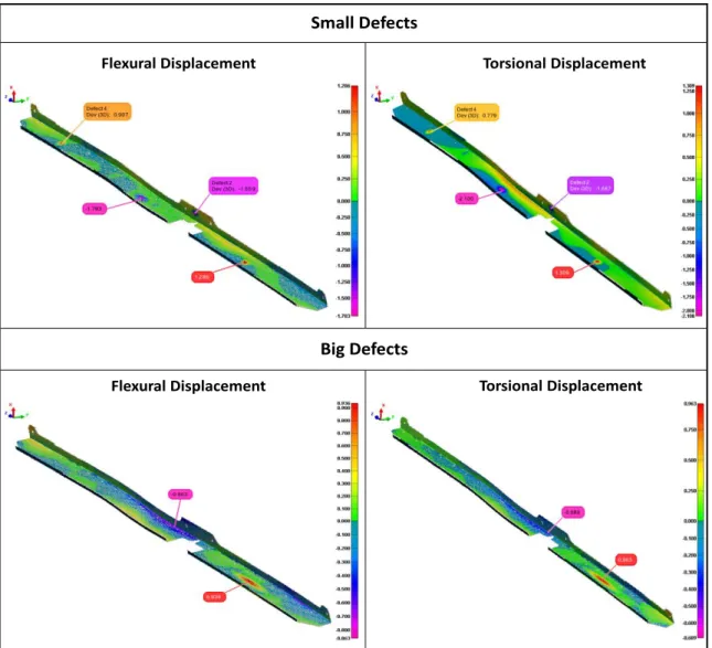
Figure 8: Defect amplitudes (mm), positions and areas, using inspection color map – Case A (original, noise-free)
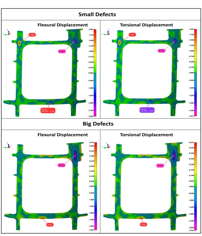
Torsional Displacement Small Defects Flexural Displacement Big Defects Torsional Displacement Flexural Displacement
Figure 9: Defect amplitudes (mm), positions and areas, using inspection color map – Case B (original, noise-free)
The error percentage generally decreases by improving the definition of boundary conditions. A precise and complete definition of boundary conditions leads to precise results. Also, the accuracy of the correspondence searching method (the modified GNIF method in our paper) definitely affects the results. The modified 64-bit version of the GNIF algorithm lets us to deal with large flexible parts with very dense point clouds. Satisfactory results can be achieved in a very short time compared to the original approach, by taking advantage of the recently developed platform for automatic node insertion and FE solver. To explain the various values of the algorithmic error in different (and even the same) defects, uncertainty sources should be identified. Regarding the different steps of the algorithm, the developed method’s accuracy is limited by the uncertainty of these elements: the correspondence search, the displacement boundary condition formulation, and the FE solver. The only known source of error is the Gaussian measurement noise added numerically for the simulation of scanned parts to study the method’s robustness. The algorithmic error is the combination of the mentioned uncertainty errors whose values are not known or predictable to us. A validation research is needed to study and quantify these uncertainties. Figure 10 illustrates the different uncertainty sources in the presented approach.
𝜎 = 0,01, 0,02, 0,03 𝑚𝑚 𝜎 =
𝜎 =
𝜎 = Gaussian measurement noise
Correspondence search Displacement boundary condition formulation FE solver mm mm
Figure 10: Different uncertainty sources in the developed algorithm
Figure 11 represents Box Plots for the results of the maximum error (%) relative to 𝜎𝑛𝑜𝑖𝑠𝑒 in each case A and B. Comparing the results in different values of 𝜎𝑛𝑜𝑖𝑠𝑒, the developed algorithm can be considered repeatable and robust to the typical measurement noise forasmuch as there is an insignificant difference between intervals respect to the different values of 𝜎𝑛𝑜𝑖𝑠𝑒. This is because the centres of mass (based on which the displacement vectors for the FE simulation are calculated) are defined as the average of the neighborhood points in each area. Therefore, the noise is quite averagely compensated in a centre of mass.
A small bias is seen in the case B that could be because of some reasons such as the part’s high length relative to its width and maybe insufficient or inaccurate definition of displacement boundary conditions and areas. This bias is not significant in the case A that is not too long relative to its width, and the boundary conditions in which are defined, in quantity and quality, better than in the case B.
CASE A
CASE B
Figure 11: Box Plots for the results of the maximum algorithmic error on profile deviation (%) relative to 𝝈𝒏𝒐 𝒔𝒆 in the cases A and B
5 CONCLUSION
In the present paper, an automatic method for the profile inspection of flexible parts was developed to eliminate the need for dedicated inspection fixtures. This approach was studied and evaluated on two industrial non-rigid part models from our industrial partner, Bombardier Aerospace Inc. To compare a point cloud (extracted from a simulated part
containing known displacement and deviations) with the CAD model, a pre-alignment and a rigid registration (using the ICP method) were done first. Then, correspondents between the two data sets were found applying our modified 64-bit version of the GNIF method. Next, knowing the constrained areas such as contact surfaces and fixation areas on the CAD model, planes were fitted through the points inside each area as well as their correspondents on the digitized data. Then, the displacement boundary conditions were completely defined by local translation laws for finite element simulation. The deviation amplitudes, areas, and positions were identified comparing the scanned data with the displaced CAD model. In this paper, the improved method was applied on two industrial flexible parts with free-form complex surfaces. A definition of boundary conditions, and consequently, an identification of deviations were improved using our approach. If the boundary conditions are completely and exactly defined, more precise results will inevitably be achieved. The 64-bit version of the GNIF algorithm made us able to apply the method on large flexible parts with dense point clouds (e.g. the case C). Accuracy of the algorithm was improved by using a sample projection technique for the formulation of displacement boundary conditions. Time was saved, compared to the original approach, using an automatic node insertion technique and FE solver. The latter allowed us to study repeatability of the proposed method by introducing Gaussian measurement noise three times on each case. Metrological performance of the approach was analysed using Box Plots that proved the robustness of the method to the typical measurement noise according to the results of the repeatability evaluation. Our research advances to implement this approach on real point clouds acquired from part surfaces in order to improve the definition of, and to consider different kinds of, boundary conditions.
6 ACKNOWLEDGMENTS
The authors would like to thank the National Sciences and Engineering Research Council (NSERC) and our industrial partners for their support and financial contribution.
7 REFERENCES
1. Gao, J., N. Gindy, and X. Chen, An automated GD&T inspection system based on non-contact 3D digitization. International journal of production research, 2006. 44(1): p. 117-134.
2. Li, Y. and P. Gu, Inspection of free-form shaped parts. Robotics and Computer-Integrated Manufacturing, 2005. 21(4-5): p. 421-430.
3. ASME-Y14.5, ASME Y14.5-2009, in Dimensioning and tolerancing2009, The American Society of Mechanical Engineers National Standard: The American Society of Mechanical Engineers, New York.
4. ISO-1101:, ISO 1101:2004, in Geometrical product specifications (GPS)—geometrical tolerancing—tolerances of form, orientation, location and run-out2004, International Organization for Standardization (ISO): Geneva.
5. ISO-10579:, ISO 10579:2010, in Geometrical product specifications (GPS)— dimensioning and tolerancing—non-rigid parts2010, International Organization for Standardization (ISO): Geneva.
6. Abenhaim, G.N., et al., A novel approach for the inspection of flexible parts without the use of special fixtures. Journal of Manufacturing Science and Engineering, 2011. 133(1).
7. Li, Y. and P. Gu, Free-form surface inspection techniques state of the art review. Computer-Aided Design, 2004. 36(13): p. 1395-1417.
8. Besl, P.J. and N.D. McKay, A method for registration of 3-D shapes. IEEE Transactions on pattern analysis and machine intelligence, 1992. 14(2): p. 239-256.
9. Borg, I. and P.J.F. Groenen, Modern multidimensional scaling: Theory and applications. 2005: Springer Verlag.
10. Myronenko, A. and S. Xubo, Point Set Registration: Coherent Point Drift. Pattern Analysis and Machine Intelligence, IEEE Transactions on, 2010. 32(12): p. 2262-2275. 11. Abenhaim, G.N., A. Desrochers, and S.A. Tahan, Nonrigid parts’ specification and
inspection methods: notions, challenges, and recent advancements. The International Journal of Advanced Manufacturing Technology, 2012. 63(5-8): p. 741-752.
12. Aidibe, A. and A. Tahan, The inspection of deformable bodies using curvature estimation and Thompson-Biweight test. The International Journal of Advanced Manufacturing Technology, 2014: p. 1-15.
13. Sabri, V., et al., Fixtureless profile inspection of non-rigid parts using the numerical inspection fixture with improved definition of displacement boundary conditions. The International Journal of Advanced Manufacturing Technology, 2016. 82(5): p. 1343-1352.
14. Ascione, R. and W. Polini, Measurement of nonrigid freeform surfaces by coordinate measuring machine. The International Journal of Advanced Manufacturing Technology, 2010. 51(9-12): p. 1055-1067.
15. Weckenmann, A. and A. Gabbia, Testing formed sheet metal parts using fringe projection and evaluation by virtual distortion compensation, in Fringe 2005, W. Osten, Editor. 2006, Springer Berlin Heidelberg. p. 539-546.
16. Weckenmann, A. and J. Weickmann, Optical inspection of formed sheet metal parts applying fringe projection systems and virtual fixation. Metrology and Measurement Systems, 2006. 13(4): p. 321-334.
17. Weckenmann, A., J. Weickmann, and N. Petrovic. Shortening of Inspection Processes by Virtual Reverse Deformation. in Proceedings of the CIRP 4th International Conference and Exhibition on Machines and Design and Production of Dies and Molds. 2007. Cesme, Izmir, Turkey.
18. Jaramillo, A.E., P. Boulanger, and F. Prieto. On-line 3-D inspection of deformable parts using FEM trained radial basis functions. in IEEE 12th International Conference on Computer Vision Workshops (ICCV Workshops). 2009. Kyoto, Japan: IEEE.
19. Jaramillo, A.E., P. Boulanger, and F. Prieto, On-line 3-D system for the inspection of deformable parts. The International Journal of Advanced Manufacturing Technology, 2011. 57(9-12): p. 1053-1063.
20. Jaramillo, A., F. Prieto, and P. Boulanger, Fast dimensional inspection of deformable parts from partial views. Computers in Industry, 2013(0).
21. Gentilini, I. and K. Shimada, Predicting and evaluating the post-assembly shape of thin-walled components via 3D laser digitization and FEA simulation of the assembly process. Computer-Aided Design, 2011. 43(3): p. 316-328.
22. Radvar-Esfahlan, H. and S.A. Tahan, Nonrigid geometric metrology using generalized numerical inspection fixtures. Precision Engineering, 2012. 36(1): p. 1-9.
23. Radvar-Esfahlan, H. and S.-A. Tahan, Robust generalized numerical inspection fixture for the metrology of compliant mechanical parts. The International Journal of Advanced Manufacturing Technology, 2014. 70(5-8): p. 1101-1112.
24. Abenhaim, G.N., et al., A Novel Approach for the Inspection of Flexible Parts Without the Use of Special Fixtures. Journal of Manufacturing Science and Engineering, 2011. 133(1): p. 011009-11.
25. Amberg, B., S. Romdhani, and T. Vetter. Optimal Step Nonrigid ICP Algorithms for Surface Registration. in IEEE Conference on Computer Vision and Pattern Recognition. 2007. Minneapolis, MN, USA.
26. Aidibe, A., A. Tahan, and G. Abenhaim, Distinguishing profile deviations from a part’s deformation using the maximum normed residual test. WSEAS Transactions on Applied and Theoretical Mechanics, 2012. 7(1): p. 18-28.
27. Aidibe, A. and A. Tahan, Adapting the coherent point drift algorithm to the fixtureless dimensional inspection of compliant parts. The International Journal of Advanced Manufacturing Technology, 2015: p. 1-11.
28. Abenhaim, G.N., et al., A virtual fixture using a FE-based transformation model embedded into a constrained optimization for the dimensional inspection of nonrigid parts. Computer-Aided Design, 2015. 62: p. 248-258.
29. Sattarpanah Karganroudi, S., et al., Automatic fixtureless inspection of non-rigid parts based on filtering registration points. The International Journal of Advanced Manufacturing Technology, 2016. 87(1): p. 687-712.
30. Thiébaut, F., et al., Evaluation of the shape deviation of non rigid parts from optical measurements. The International Journal of Advanced Manufacturing Technology, 2017. 88(5): p. 1937-1944.
31. Borouchaki, H., P.L. George, and S.H. Lo, Optimal delaunay point insertion. International Journal for Numerical Methods in Engineering, 1996. 39(20): p. 3407– 3437.
32. Cuillière, J.-C. and V. Francois, Integration of CAD, FEA and Topology Optimization through a Unified Topological Model. Computer-Aided Design and Applications, 2014. 11(5): p. 493-508.