HAL Id: hal-00925313
https://hal.inria.fr/hal-00925313
Submitted on 7 Jan 2014
HAL is a multi-disciplinary open access
archive for the deposit and dissemination of
sci-entific research documents, whether they are
pub-lished or not. The documents may come from
teaching and research institutions in France or
L’archive ouverte pluridisciplinaire HAL, est
destinée au dépôt et à la diffusion de documents
scientifiques de niveau recherche, publiés ou non,
émanant des établissements d’enseignement et de
recherche français ou étrangers, des laboratoires
Energy efficiency in HPC with and without knowledge
of applications and services
Mohammed El Mehdi Diouri, Ghislain Landry Tsafack Chetsa, Olivier Glück,
Laurent Lefevre, Jean-Marc Pierson, Patricia Stolf, Georges da Costa
To cite this version:
Mohammed El Mehdi Diouri, Ghislain Landry Tsafack Chetsa, Olivier Glück, Laurent Lefevre,
Jean-Marc Pierson, et al.. Energy efficiency in HPC with and without knowledge of applications and
services. International Journal of High Performance Computing Applications, SAGE Publications,
2013, 27 (3), pp.232-243. �10.1177/1094342013495304�. �hal-00925313�
Energy efficiency in HPC with and without
knowledge of applications and services
M. E. M. Diouri
1, G. L. Tsafack Chetsa
1,2, O. Gl¨
uck
1, L. Lef`evre
1,
J.-M. Pierson
2, P. Stolf
2, and G. Da Costa
21
INRIA Avalon Team, LIP Laboratory (UMR CNRS, ENS,
INRIA, UCB), Ecole Normale Sup´erieure de Lyon, Universit´e de
Lyon, France, Email: {mehdi.diouri, ghislain.landry.tsafack.chetsa,
olivier.gluck, laurent.lefevre}@ens-lyon.fr
2
IRIT (UMR CNRS), University of Toulouse, 118 Route de
Narbonne, F-31062 Toulouse CEDEX 9, France, Email: {pierson,
stolf, dacosta}@irit.fr
Abstract
The constant demand of raw performance in high performance com-puting often leads to high performance systems’ over-provisioning which in turn can result in a colossal energy waste due to workload/application variation over time. Proposing energy efficient solutions in the context of large scale HPC is a real unavoidable challenge. This paper explores two alternative approaches (with or without knowledge of applications and services) dealing with the same goal: reducing the energy usage of large scale infrastructures which support HPC applications. This article describes the first approach ”with knowledge of applications and services” which enables users to choose the less consuming implementation of ser-vices. Based on the energy consumption estimation of the different imple-mentations (protocols) for each service, this approach is validated on the case of fault tolerance service in HPC. The approach ”without knowledge” allows some intelligent framework to observe the life of HPC systems and proposes some energy reduction schemes. This framework automatically estimates the energy consumption of the HPC system in order to apply power saving schemes. Both approaches are experimentally evaluated and analyzed in terms of energy efficiency.
1
Introduction
High performance computing (HPC) systems are used to run a wide range of scientific applications from various domains including cars and aircraft design, prediction of severe weather phenomena and seismic waves. To enable this,
there is a constant demand of raw performance in HPC systems which often leads to their over-provisioning which in turn can result in a colossal energy waste due to workload/application variation over time. Energy consumption becomes a major problem as we live now in an energy-scarce world; and HPC centers have an important role to play due to the rise of scientific needs. This is evidenced by the Green5001
list, which provides a ranking of the greenest HPC systems around the world as opposed to the Top5002
which emphasizes the performance of those systems. Consequently, designing energy efficient solutions in the context of large scale HPC is a real unavoidable challenge.
This article explores two approaches for supporting energy efficiency in HPC systems, the first approach assumes complete knowledge of applications and services whereas the second does not. However, they are complementary and serve the same goal: intelligently estimating resource and energy usage before applying green levers (shutdown/slowdown) in order to reduce the electrical usage of large scale HPC infrastructures.
In the era of petascale and yet to come exascale infrastructures, design-ing scalable, reliable, and energy efficient applications remains a real challenge. HPC applications along with associated services (fault tolerance, data manage-ment, visualization...), can become difficult to program and optimize. Thanks to the programmer’s expertise about designed applications and services, we can avoid over provisioning of resources during the life of HPC infrastructures.
Designers seeking to reduce the energy usage should be helped in choosing adequate protocols, services and the best implementations of their applications with regards to the targeted infrastructure. In other words, evaluating and estimating the energy impact of applications and services can help users in choosing a more energy efficient version of the application at hand. This paper presents a methodology and a framework which allows energy usage estimations of a set of HPC services. Thanks to these estimations, the framework can help users to determine the least consuming version of the services depending on their application requirements. To validate our framework, real experiments on a set of protocols of the fault tolerance service are proposed and analyzed.
Alternatively, one can suggest that designing large scale HPC applications and services is becoming too complex and difficult. Exploring autonomous solu-tions able to propose and apply energy reduction solusolu-tions must be investigated. Several scientific applications throughout their life-cycle exhibit diverse behav-iors also known as phases. These phases are not only similar because of their resource utilization pattern, the energy consumed by the application in different phases is likely to be different as well.
As a second major contribution of this paper, we present and implement an on-line methodology for phase detection and identification in HPC systems without having any knowledge of the running applications. The approach tracks phases, characterizes them and takes advantage of our partial phase recognition technique. It automatically applies power saving schemes in order to improve
1
Green500 Lists: http://www.green500.org 2
energy efficiency of the HPC system. Validations with a set of selected applica-tions are presented and analyzed.
The remainder of the paper is organized as follows: section 2 describes con-sidered approach when some knowledge is available on applications and services. This section focuses on the Fault Tolerance service in HPC. Section 3 analyses the alternative approach where energy efficiency can be obtained in an auto-matic external approach when no knowledge is available on the applications. Finally, section 4 concludes this paper.
2
Energy efficiency in HPC with knowledge of
applications and services
Large scale HPC applications need to meet with several challenges (fault tol-erance, data processing, etc.). In order to overcome these challenges, several services need to be run harmoniously together with extreme-scale scientific ap-plications.
In our study, we identify the following services:
• Checkpointing: Performed during the normal functioning of the applica-tion, it consists in storing a snapshot image of the current application state;
• Recovery: In case of failure, it consists in restarting the execution of the application from the last checkpoint;
• Data exchanges: Scattering data over several processes; Broadcasting data to all processes; Gathering data over several processes; Retrieving a spe-cific data among all processes;
• Visualizing the application logs in real time;
• Monitoring the hardware resources that are involved in the extreme-scale system.
For each service presented above, several implementations are possible. Even if our approach aims to cover all kinds of applications and all the services, this section focuses on the checkpointing service as an example [1]. As concerns checkpointing, applications can be run either with coordinated, uncoordinated, or hierarchical checkpointing. These protocols rely on checkpointing and in order to obtain a coherent global state, this checkpointing is associated with message logging in uncoordinated protocols [2] and with process coordination in coordinated protocols [3]. Hybrid protocols propose to use coordinated protocol within the same cluster and message logging for messages exchanged between clusters [4]. In uncoordinated protocols, the crashed processes are re-executed from their last checkpoint image to reach the state immediately preceding the crashing state in order to recover a coherent state with non crashed processes
[5]. In coordinated protocols, all the processes must rollback to the previous coherent state, meaning to the last full completed coordinated checkpointing.
The less energy consuming fault tolerance protocol is not always the same depending on the executed application and on the execution context. Thus, to consume less energy is to let the user choose the less consuming protocol. To this end, we propose to take into account the application features and the user requirements in order to provide an energy estimation of the different imple-mentations of the services required by the user [6].
Making an accurate estimation of the energy consumption due to a specific implementation of a given service is really complex as it depends on several parameters that are related not only to the protocols but also to the applica-tion features, and to the hardware used. Thus, in order to accurately estimate the energy consumption due to a specific implementation of a fault tolerance protocol, our energy estimator needs to take into consideration all the proto-col parameters (checkpointing interval, checkpointing storage destination, etc.), all the application specifications (number of processes, number and size of ex-changed messages, volume of data written/read by each process, etc.) and all the hardware parameters (number of cores per node, memory architecture, type of hard disk drives, etc.). We consider that a parameter is a variable of our estimator only if a variation of this parameter generates a significant variation of the energy consumption while all the other parameters are fixed. In order to take into consideration all the parameters, our estimator incorporates an automated calibration component.
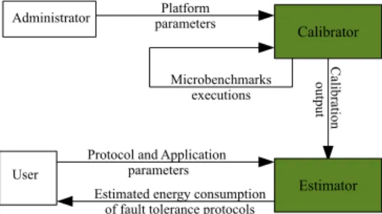
Figure 1 shows the components of our estimator framework and their inter-actions. As an input, the estimator component gathers information related to the execution context and to the application the user would like to run. As an output, the calibrator component provides the calibration data on which our framework relies on to estimate the energy consumption of services.
Finally, in order to achieve important energy savings, we propose to shut-down or slowshut-down resources during their idle and active waiting periods. The shutdown approach is promoted only if the idle or active waiting period is long enough, greater than the minimum threshold from which it becomes gainful to turn off a resource and turn it on again [7]. The shutdown and slowdown approaches are proposed at the component level, meaning that we consider to switch off or slowdown CPU/GPU cores, network interfaces, storage medium.
2.1
Calibration approach
The goal of the calibration process is to gather energy knowledge of all the identified operations (e.g. checkpointing, coordination, logging, etc.) according to the hardware used in the supercomputer. Indeed, the energy consumption of a fault tolerance protocol may be different depending on the hardware used. The goal of our calibration approach is to take into consideration in our energy estimations the specific hardware used.
A basic operation is a task op which is characterized by a constant power consumption. To this end, a set of simple benchmarks extract the energy
con-sumption Eop of the basic operations encountered in the different versions of a
same service. The energy consumption of a node i performing a basic operation opis: Eiop= P
op i · t
op i .
topi is the time required to perform op by the node i. Piop is the power
consumption of the node i during topi . Thus, for each node i, we need to get the
power consumption Piop, and the execution time t op
i of each basic operation.
The power consumption of an operation op is: Piop= P idle
i + ∆P
op i .
Pidle
i is the power consumption when the node i is idle and ∆P op
i is its extra
power consumption due to the basic operation. In our paper [8], we showed that Pidle
i may be different even for identical nodes. Thus, we calibrate Piidleby
measuring the power consumption of each node while it is idle. In addition, we measure ∆Piop for each node i and during each basic operation op. In order to
measure ∆Piopexperimentally, we isolate each basic operation by instrumenting
the implementation of each version of the service that we consider, and we use a power meter which provides up power measurements with a high sampling rate (e.g, 1 measurement per second).
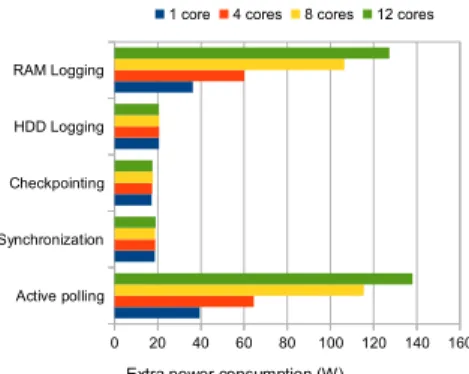
To put it into perspective, we provide the calibration results of a cluster con-stituted of 16 nodes Dell R720. Each node contains 2 Intel Xeon CPU 2.3 GHz, with 6 cores each; 32 GB of memory; a 10 Gigabit Ethernet network; a SCSI hard disk with a storage capacity of 598 GB. First, we measure the idle power consumption of each node (Figure 2), then we measure the extra power con-sumption ∆Piopof all the basic operations found in the fault tolerance protocols
(Figure 3). In order to collect such power measurements, we used an energy-sensing infrastructure of external power meters from the SME Omegawatt. This energy-sensing infrastructure enables to get the instantaneous consumption in Watts, at each second for each monitored node [9]. As each node has 12 cores each, we calibrated the extra power cost by assuming that 1, 4, 8 or 12 processes are running the same operation at the same time.
Protocol and Application parameters C al ibr at ion out put
Estimated energy consumption of fault tolerance protocols
Calibrator Platform parameters Estimator User Administrator Microbenchmarks executions
Figure 1: Estimator components and interactions Figure 2 confirms that Pidle
i is different for identical nodes. This highlights
the need to perform such power calibration even for nodes within the same clus-ter. Figure 3 shows the mean extra power measurements over all the nodes. Compared to the average values plotted in Figure 3, the variances are very low.
1 2 3 4 5 6 7 8 9 10 11 12 13 14 15 16 93 94 95 96 97 98 99 100 101 102 Cluster nodes
Idle power consumption (W)
Figure 2: Idle Power Measurements
Active polling Synchronization Checkpointing HDD Logging RAM Logging 0 20 40 60 80 100 120 140 160 1 core 4 cores 8 cores 12 cores
Extra power consumption (W)
Figure 3: Mean Extra Power Mea-surements
This suggests that ∆Piop is almost the same for the nodes of the cluster that
we monitored. Figure 3 also shows that the most power consuming operations are the RAM logging and the active polling that occurs during the coordina-tion if processes are not synchronized. We also notice that for these two basic operations, the extra power consumption varies with the number of cores per node that perform the same operation. This is because more cores are running intensively for these two operations.
For each operation op, topi depends on different parameters. For a given node
i, the time required for checkpointing a volume of data, of for logging a message is: topi = t access i + t transf er i = t access i + Vdata rtransf eri (1)
taccessi is the time to access the storage media where the checkpoint will be
stored. ttransf eri is the time to write a data on a given storage media. r transf er i
is the transmission rate of the storage media. taccess i and r
transf er
i are almost
constant when we consider volumes of data of the same order of magnitude. The coordinated checkpointing at the system level requires an extra synchro-nization between the processes. Therefore, the time for a process coordination is: topi = t polling i + t synchro= V data rtransf eri + t synchro (2)
tsynchro is the time to exchange a marker among all the processes. tsynchro
depends on the number of processes to synchronize and the number of processes per node. tpollingi is the time necessary to finish transfers of inflight messages at
the coordination time.
In order to calibrate topi , our estimator automatically runs a simple
bench-mark that measures the execution time for different varying parameters, namely Vdata.
In order to take into consideration the eventual contention that may occur on the same storage media, we also perform this calibration for different numbers of processes per node which are running the same operation at the same time. We perform this calibration process for all the different storage medium (RAM, HDD, SSD, ...) that are available in the supercomputer.
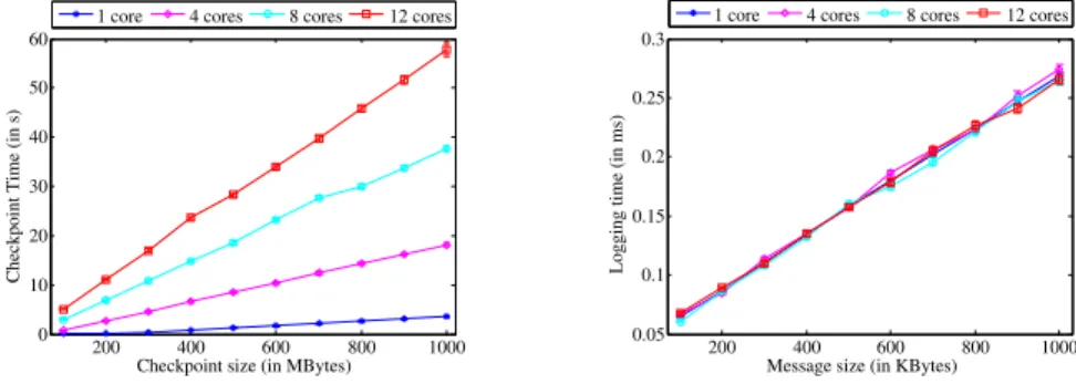
Figures 4, 5 and 6 present the calibration of topi for the 16-nodes cluster
considering different basic operations: checkpointing on HDD, message logging on RAM and process synchronization. In Figures 4 and 5 are also represented the standard deviations (error bars) due to the computation of the average values over all the nodes of our cluster. These standard deviations are invisible since the differences between the checkpointing and logging times all over the nodes are insignificant.
200 400 600 800 1000 0 10 20 30 40 50 60
Checkpoint size (in MBytes)
Checkpoint Time (in s)
1 core 4 cores 8 cores 12 cores
Figure 4: tcheckpoint calibration
200 400 600 800 1000 0.05 0.1 0.15 0.2 0.25 0.3
Message size (in KBytes)
Logging time (in ms)
1 core 4 cores 8 cores 12 cores
Figure 5: tlogging calibration
1 2 3 4 5 6 7 8 9 10 11 12 13 14 15 16 0 0.005 0.01 0.015 0.02 0.025 0.03 0.035 0.04 Number of nodes
Synchronization Time (in s)
1 core 4 cores 8 cores 12 cores
Figure 6: tsynchrocalibration
From Figure 4, we notice that when several cores are logging at the same time, the execution time is higher: simultaneous accesses on HDD create I/O contentions. That is the reason why we need to calibrate the execution time for different numbers of processes per node. As concerns message logging on RAM, we observe in Figure 5 that logging time does not vary when the number of cores per node is changed. This is because there is no contention when several cores do RAM access simultaneously.
Figure 6 shows that the synchronization time is slightly higher when we consider more processes per node. Synchronizing processes that are on the same node requires much less time than processes on distinct nodes. This is due to the network transmission rate that is much lower than the transmission rate within the same node.
2.2
Estimation methodology
Once this calibration is completed, our framework can estimate the energy con-sumption of the different versions of the studied service. For each operation op, topi depends on different parameters related to the application and the
execu-tion context. This informaexecu-tion is collected from the user as an input by the calibrator.
To estimate the energy consumption of checkpointing, the estimator com-ponent collects from the user the total memory size required by the application to run, the total number of nodes and the number of processes per node. From this information, the estimator computes the mean memory size Vmem
mean required
by each node. The estimator also collects the number of checkpoints to perform during the application execution. In addition, it collects from the calibrator the checkpoint times corresponding to the calibrated checkpoint sizes. The es-timator calculates the checkpoint times tcheckpointi corresponding to Vmeanmem. As
shown in Section 2.1, most of the execution time models are linear. Therefore, if Vmem
mean is not the size recorded by the calibrator, the estimator computes the
equation that gives tcheckpointi according to V mem
mean, and adjusts the equation
us-ing the linear least squares method [10]: y = αx+β. In the case of checkpointus-ing operation, α is taccess
i while β is 1
rtransf eri . x is V data.
To estimate the energy consumed by message logging, the estimator collects from the user the number of processes per node, the total number and size of the messages sent during the application. From this information, it computes the mean volume of data Vmean
data sent (so logged) by each node. Similarly to
check-pointing, it collects from the calibrator the logging time ti
logging corresponding
to Vmean
data for each node and according to the number of processes per node.
To estimate the energy consumed by coordination, the estimator uses the mean message size Vmean
message as the total size of messages divided by the total
number of messages. It also uses the number of checkpoints C, the total number of nodes N and the number of processes per node that are provided for message logging and checkpointing estimations. From the calibration output, it collects the synchronization time tsynchrocorresponding to the number of processes per
node and the total number of nodes specified by the user. tsynchrocorresponds
to one synchronization among all the processes. Similarly to checkpointing, the estimator calculates the message transfer time ti
polling corresponding to the
mean message size Vmean message.
The estimated energy of one basic operation op (checkpointing, logging, polling or synchronization) is:
Eop=PNi=1E op i = PN i=1P op i · t op i
The total estimated energy consumption of checkpointing is obtained by multiplying Echeckpoint by the number of checkpoints C. The estimated energy
of all coordinations is calculated as follows:
Ecoordinations= C · (Epolling+ Esynchro).
To estimate the energy consumed by hierarchical checkpointing, the estima-tor collects from the user the composition of each cluster (i.e the list of processes in each cluster).
We can obtain the overall energy estimation of the entire checkpointing pro-tocol from the sum of the sub-components energy consumptions. Indeed, check-pointing is a common basic operation for both coordinated, uncoordinated and hierarchical protocols. If we add the energy consumed by the checkpointing to the energy consumption of message logging, we obtain the overall energy con-sumption of uncoordinated checkpointing. If we add the energy concon-sumption of checkpointing to the energy consumption of coordinations, we obtain the overall energy consumption of coordinated checkpointing.
2.3
Validation of the estimation framework
In this section, we want to compare the energy consumption obtained by our estimator once the calibration is done (but before running the application) to the real energy consumption measured by our energy sensors during the application execution. For these experiments, we use the same cluster as the one described in Section 2.1.
We consider 4 HPC applications running over 144 processes (i.e. 12 nodes with 12 cores per node): CM13
with a resolution of 2400x2400x40 and 3 NAS 4
in Class D (SP, BT and EP). For each application, we measure the total energy consumption of one application execution with and without the basic opera-tions activated in the fault tolerance protocols. To this end, we instrumented the code of fault tolerance protocols and we obtain the energy consumption of each operation. Each energy measurement is done 30 times and we compute the average value. For checkpointing measurements, we consider a checkpoint interval of 120 seconds.
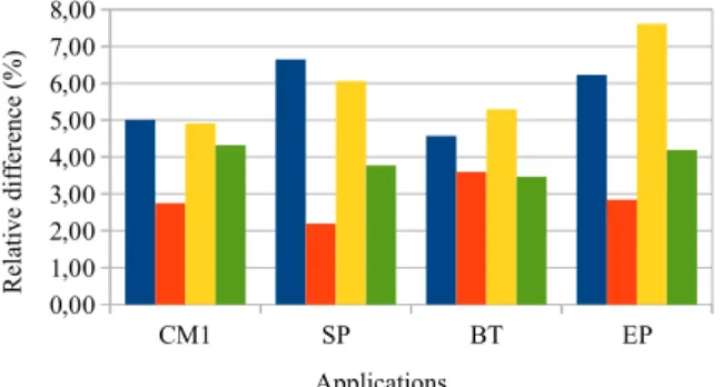
In Figure 7, we compare our energy estimations to real measurements, the relative differences between the estimated and the measured energy consump-tions are low. Indeed, the worst relative difference that we obtain is 7.5 %. This shows that our energy estimations are accurate. This estimation error may be attributed partly to the proposed estimation method but also partly to the measurement error. By providing the average values over 30 measurements, we aimed at reducing the impact of the measurement error.
In Figure 8, we plot the estimated energy consumption computed by our framework for each basic operation and for each application considered. Figure 8 shows that energy consumption of one operation is not the same from one
3
Cloud Model 1: http://www.mmm.ucar.edu/people/bryan/cm1/ 4
ng CM1 SP BT EP 0,00 1,00 2,00 3,00 4,00 5,00 6,00 7,00 8,00
RAM Logging HDD Logging Coordination Checkpointing
Applications R el at ive d if fe re nc e ( % )
Figure 7: Relative difference (in %) between the estimated and the measured energy consumption 51,48 Joules 09,51 Joules 945515,62 CM1 SP BT EP 0,0 50,0 100,0 150,0 200,0 250,0 300,0 4 ,3 4 3 ,6 2 3 ,0 0 ,4 2 3 ,2 1 7 9 ,0 1 1 1 ,2 2 ,4 2 ,3 4,6 2 ,6 4,3 2 5 3 ,8 2 0 8 ,9 1 2 4 ,1 1 2 ,1
RAM Logging HDD Logging Coordination Checkpointing
Applications E st im at ed ene rgy c ons um p ti on ( kJ )
Figure 8: Estimated energy consumption (in kJ) of high-level operations
application to another. For instance, the energy consumption of RAM logging in SP is more than the one in EP. In addition, HDD checkpointing in CM1 is 20 times more than in EP.
2.4
Determination of the least consuming version of a
given service
The results presented in section 2.3 allow us to address the following question: how our estimator framework can help selecting the lowest energy consuming version of the considered service ? To answer this question, the case of the checkpointing service is also taken as an example.
As mentioned before, both uncoordinated and coordinated protocols rely on checkpointing. Checkpointing is combined with message logging in uncoor-dinated protocols and with coordination in cooruncoor-dinated protocols. Therefore,
to compare coordinated and uncoordinated protocols from an energy consump-tion standpoint, we compare the extra energy consumpconsump-tion of coordinaconsump-tion to message logging.
From one application to another the lowest energy consuming protocol is not always the same (see Figure 8). Indeed, for BT, SP and CM1, the less energy consuming protocol is the coordinated protocol since the volume of data to log for these applications is relatively important whereas it is the coordinated protocol with RAM logging for EP. We also notice that for applications we considered, the uncoordinated protocol with HDD logging is always more energy consuming than the coordinated protocol. By providing such energy estimations before executing the HPC application, we can select the best fault tolerant protocol in terms of energy consumption.
3
Energy efficiency in HPC without knowledge
of the applications
High performance computing (HPC) systems users generally seek better perfor-mance for their applications; consequently, any management policy that aims at reducing the energy consumption should not degrade performance. To mitigate performance degradation while improving energy performance, it is mandatory to understand the behavior of the system at hand at runtime. Put simply, opti-mization proposed is closely related to the behavior of the system. For instance, scaling the CPU frequency down to its minimum when running CPU-bound workloads may cause significant performance degradation, which is unaccept-able. Thus, to efficiently optimize a HPC system at runtime, it is necessary to identify the different behaviors known as phases during execution. In this section, we discuss our phase identification approach along with management policies.
The rational behind this work is that it is possible to improve energy perfor-mance of a system with nearly no perforperfor-mance degradation by carefully selecting power saving schemes to apply to the system at a given point in time. Several classical well known techniques set the CPU frequency according to estimated usage of the processor over a time period [11, 12, 13, 14, 15]. We believe that actions on the system at runtime can result in energy savings provided they are carefully selected. For instance, adjusting the frequency of the processor or the speed of the network interconnect (NIC), switching off memory banks, spinning down disks, and migrating tasks among nodes of the system, are ways of adjusting the system to the actual demand (or applications’ requirements) at runtime.
From what precedes, choosing the appropriate lever (power saving scheme) is critical; an effective way of choosing between the different levers is to first characterize phases or system’s behaviours so that similar phase patterns can easily be identified with each other. So doing, a set of power saving schemes deemed efficient both in terms of energy and performance for a given phase can
be used for recurring phases. This is accomplished by associating a set of levers to each characterized phase. Details with regards to phase characterization are provided in Section 3.1.
Once phases are characterized, the next step boils down to identifying (still at runtime) recurring phases in order to apply adequate power saving schemes. To accomplish this, we use an approach which we refer to as partial phase recognition. Instead of trying to recognize a complete phase prior to adjusting the system (which might lead to an unexpected outcome, for the phase is already finished), we decide to adjust the system when a certain fraction of a phase has been recognized. This technique is clearly giving false positives (an ongoing phase is recognized as part of a known phase in error), but we argue that the adjustment of the system is beneficial at least for a certain time. When the ongoing phase diverges too much from the recognized phase, another phase can be identified or a new phase characterized. Phase identification and partial recognition are detailed in Section 3.2.
3.1
Phases tracking and characterizing
Our methodology relies on the concept of execution vector (EV) which is similar to power vectors (PV) [16]. An execution vector is a column vector whose entries are system’s metrics including hardware performance counters, network byte sent/received and disk read/write counts. For convenience, we will refer to these system’s metrics as sensors in the rest of the paper. Sensors related to hardware performance counters represents the access rate to a specific hardware register over a given time interval. Likewise, network and disk related sensors monitor network and disk activities respectively. We refer to the literature for selecting sensors related to hardware performance counters, these include: number of instructions, last level cache accesses and misses, branch misses and predictions, etc. The sampling rate corresponding to the time interval after which each sensor is read depends on the granularity. While a larger sampling rate may hide information regarding the system’s behavior, a smaller sampling rate may incur a non negligible overhead. In this work we use a sampling rate of one second. In addition, each execution vector is timestamped with the time at which it is sampled.
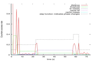
The Manhattan distance between two points in an n-dimensional space is the distance between them if a grid-like path is followed. It offers the advantage that it does not depend on the translation of the coordinate axes with respect to a coordinate axis, i.e., it weights more heavily differences in each dimension. Properties just mentioned motivate our use of the Manhattan distance as the resemblance or similarity metric between execution vectors. This similarity is used to cluster EVs along the execution time-line as follows: two consecutive EVs along the execution time-line belong to the same group or are similar if the Manhattan distance between them is bellow a similarity threshold (denoted as ST in the following). We define the similarity threshold as a percentage of the maximum known distance between all consecutive execution vectors (along the execution time line). For example, given a similarity threshold of 10%, two
0 0.2 0.4 0.6 0.8 1 0 10 20 30 40 50 60 70
Counters access rate
time (s) distance threshold br misses cache ref cache misses step function: indicates phase changes
Figure 9: Phase identification using similarities between consecutive EVs; steps of the step function indicate phase changes.
consecutive EVs belong to the same group if the Manhattan distance between them is less than 10% of the maximum existing distance between all consecutive execution vectors.
Knowing that the behaviour of the system is relatively stable during a phase and assuming that stability is translated into execution vectors sampled during the phase, we define a phase as any behaviour delimited by two successive Man-hattan distances exceeding the similarity threshold. Therefore, let’s consider the graphic of Figure 9, where the x-axis represents the execution time-line; with a similarity threshold of 15%, we can observe 5 phases as indicated by the step function. Note that the threshold varies throughout the system’s life time since the maximum existing vector is re-initialized once a phase is detected. It can be seen in Figure 9 that a phase change is detected when the Manhattan distance between two consecutive EVs exceeds the threshold (which is 15% of the maximum distance between consecutive EVs from the moment at which the last EV of the previous phase was sampled). We can also observe that these phases correspond to variations reported in the access rate of plotted per-formance counters (only a few perper-formance counters is plotted for the sake of clarity). For this experiment, the system was running a synthetic benchmark which successively runs IS and EP from NPB-3.3 [17].
The rationale behind phase tracking is the use of characteristics of known phases for optimizing similar phases. An effective phase characterization is therefore needed. To this end, once a phase is detected, we apply principal component analyses (PCA) on the dataset composed of EVs pertaining to that phase. We next keep five sensors among those contributing the least to the first principal axis (FPA) of PCA. Those five sensors serve as characteristic of the corresponding phase. PCA is a variable reduction procedure, and is used for identifying variables that shape the underlying data. In principal compo-nent analysis, the first principal compocompo-nent explains the largest variance, which
0 % 20 % 40 % 60 % 80 % 100 % WRF-ARW BT SP LU
Normalized energy consumption
performance phase-detect on-demand
(a) Average energy consumed by each application under different configu-rations. 0 % 20 % 40 % 60 % 80 % 100 % WRF-ARW BT SP LU Normalized performance
(b) Normalized performance of each application under different configurations (less than 100% means perfor-mance degradation).
Figure 10: Phase tracking and partial recognition guided processor adaptation results (They are averaged over 20 executions of each workload under each system configuration; they are normalized with respect to baseline execution “on demand”.).
intuitively means that it contains the most information and the last principal component/axis the least. Therefore, we assume that the most important vari-ables are those that contribute the most to the first principal component or axis. In other words, the most-contributing variables shape the underlying data, as opposite to the least-contributing variables which do not. But the fact that the least contributing variables do not shape the underlying data is also interesting because they eventually shape what is not in the underlying data. Thus, rely-ing on this, we assume that information regardrely-ing what the system did not do during a phase can be easily retrieved from sensors contributing the least to the first principal axis of PCA (since they are meaningless to that phase). A phase
is therefore characterized by the 5 sensors among those contributing the least to the FPA of PCA. These 5 sensors are not always the same, since the least contributing sensors depend on the activity of the system during the phase. In addition, we summarize each newly detected phase using the closest vector to the centroid of the group of vectors sampled during that phase. The closest vector to the centroid of the group of EV sampled during a phase is referred to as its reference vector.
3.2
Partial phase recognition and system adaptation
A phase cannot be detected unless it is finished, in which case any system adaptation or optimization accordingly is no longer worthwhile. The literature recommends phase prediction. Predicting the next phase permits adapting the system accordingly. Although phase prediction is very effective in some cases, it is not relevant in this context, for we do not have any a priori knowledge of applications sharing the platform. To overcome this limitation, we use partial phase recognition.
Partial phase recognition consists of identifying an ongoing phase (the phase has started and is not yet finished) Pi with a known phase Pj only considering
the already executed part of Pi. The already executed part of Pi expressed
as a percentage of the length (duration) of Pj is referred to as the recognition
threshold RT . Thus, with a RT % recognition threshold, and assuming that the reference vector of Pj is EVPj and that its length is nj, an ongoing phase Pi is identified with Pj if the Manhattan distance between EVPj and each EV pertaining to the already executed part of Pi (corresponding in length to RT %
of nj) are within the similarity threshold ST .
As an use case of our phase tracking methodology, we use the coupling of phase tracking and partial phase recognition to guide on-the-fly system adapta-tion considering the processor. We define three computaadapta-tional levels according to the characteristics of the workload: ”high” for compute intensive workload, ”medium” for memory intensive workloads and ”low” for non memory/non com-pute intensive workloads.
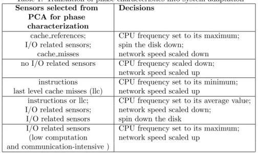
As mentioned earlier in this paper, principal component analysis (PCA) is applied to vectors belonging to any newly created phase for selecting five sensors which are used as phase characteristics. These characteristics are translated into system adaptation as detailed in Table 1. Let’s comment a few entries of that table: workloads/applications with frequent cache references and misses are likely to be memory bound. In our case, having these sensors (cache reference and cache misses) selected from PCA indicates that the workload is not memory bound. If in addition that workload does not issue a high I/O rate (presence of I/O related sensors in the first column), then we assume that it is CPU-bound; consequently, the frequency of the processor can be scaled to its maximum, the disk sent to sleep and the speed of the interconnect scaled down. For the second line of Table 1, the characteristics do not include any I/O related sensor, this implies that the system was running an I/O intensive workload; thus, the processor’s speed can be set to its minimum. Note in passing that changing the
Table 1: Translation of phase characteristics into system adaptation Sensors selected from Decisions
PCA for phase characterization
cache references; CPU frequency set to its maximum; I/O related sensors; spin the disk down;
cache misses network speed scaled down no I/O related sensors CPU frequency scaled down;
network speed scaled up
instructions CPU frequency set to its minimum; last level cache misses (llc) network speed scaled up
instructions or llc; CPU frequency set to its average value; I/O related sensors; network speed scaled down;
I/O related sensors spin down the disk
I/O related sensors CPU frequency set to its maximum; (low computation network speed scaled up
and communication-intensive )
disk’s state from sleep to active does not appear in Table 1, this is because the disk automatically becomes active when accessed.
3.3
Experimental validations
Our evaluation support is a fifteen nodes cluster set up on the Grid5000 [18] french large scale experimental platform. Each node is an Intel Xeon X3440 with 4 cores and 16 GB of RAM with frequencies ranging from 1.20 GHz to 2.53 GHz. In our experiments, low computational level always sets the CPU frequency to the lowest available (1.20 GHz), whereas high and medium computational levels set the CPU frequency to the highest available (2.53 GHz) and 2.00 GHz respectively. Each node uses its own hard drive which supports active, ready and standby states. Infiniband-20G is used for interconnecting nodes. The Linux kernel 2.6.35 is installed on each node where perf event is used to read the hardware monitoring counters. MPICH is used as MPI library. Lower-Upper Gauss-Seidel solver (LU), Scalar Penta-diagonal solver (SP), and Block Tri-diagonal solve (BT) from NPB-3.3 and a real life application, the Advance Research WRF (WRF-ARW) [19] model, are used for the experiments. Class C of NPB benchmarks are used (compiled with default options). WRF-ARW is a fully compressible conservative-form non-hydrostatic atmospheric model. It uses an explicit time-splitting integration technique to efficiently integrate the Euler equation. We monitored each node power usage with one sample per second using a power distribution unit.
To evaluate our management policy, we consider 3 basic configurations of the monitored cluster: (i) On-demand configuration in which the Linux’s“on-demand” CPU frequency scaling governor is enabled on all the nodes of the
cluster; (ii) the ”performance” configuration sets each node’s CPU frequency scaling governor to “performance”; (iii) the “phase-detect” configuration cor-responds to the configuration in which we detect phases, identify them using partial recognition and apply green levers accordingly. Figure 10(a) presents the normalized average energy consumption of the overall cluster for each ap-plication under the three cluster’s configurations. Whereas Figure 10(b) shows their execution time respectively. The results are normalized with respect to the baseline execution (on demand) and averaged over 20 executions of each workload in each configuration. Figure 10(a) and Figure 10(b) indicate that our management policy (phase-detect) consumes in average 15% less energy than ”performance” and ”on-demand” while offering the same performance for the real life application WRF-ARW. For LU, BT and SP the average energy gain ranges from 3% to 6%. Overall, the maximum amount of possible energy sav-ings depends on the workload at hand and was 19% for WRF-ARW. We are currently investigating whether we can do better with complete knowledge of the application.
From Figure 10(b), we notice a performance loss of less than 3% for LU and BT (performances are evaluated in terms of execution time). Bad performance with benchmarks come from the fact that some phases were wrongly identified as being memory intensive. Nevertheless, these results are similar to those observed in earlier work [20]. In addition, these applications do not offer much opportunities for saving energy without degrading performance. Contrarily, the numerical weather forecast model (WRF-ARW) has load imbalance which can help to reduce its energy consumption without a significant impact on its performance (in terms of execution time) [21, 22].
Above results demonstrate the effectiveness of our system’s energy manage-ment scheme based on phase detection and partial recognition. Our system performs better than a Linux’s governor because Linux’s on-demand governor will not scale the CPU frequency down unless the system’s load decreases below a threshold. The problem at this point is that the CPU load generally re-mains very high for memory intensive workloads/phases that do not require the full computational power. In this particular scenario, network and disk bound phases are too short (from milliseconds to a few seconds) and are often consid-ered as boundaries of memory or compute intensive phases. For this reason, we turned our focus to the processor. Therefore, the energy reduction mainly come from scaling the CPU down in phases suspected to be memory bound.
4
Conclusion
Energy efficiency is becoming one of the mandatory parameters that must be taken into account when operating HPC systems. In this paper, we describe and analyze some approaches to reduce the energy consumed by high perfor-mance computing systems at runtime. HPC applications and services becoming increasingly complex and difficult to program in the era of petascale and yet to come exascale; application designers have to face with resource usage, stability,
scalability and performance.
This paper shows the importance of helping users in making the right choices in terms of energy efficient services. We present a framework that estimates the energy consumption of fault tolerance protocols. In our study, we consider the three families of fault tolerance protocols: coordinated, uncoordinated and hi-erarchical protocols. To provide accurate estimations, the framework relies on an energy calibration of the execution platform and a user description of the execution settings. Thanks to our approach based on a calibration process, this framework can be used in any energy monitored supercomputer. We showed in this paper that the energy estimations provided by the framework are accu-rate. By estimating the energy consumption of fault tolerance protocols, such framework allows selecting the best fault tolerant protocol in terms of energy consumption without pre-executing the application. A direct application of our energy estimating framework is the energy consumption optimization of fault tolerance protocols.
Additionally, proposing solutions that could apply power saving schemes (shutdown or slowdown of resources) without human intervention and knowledge is a promising approach for automatic large scale energy reduction. This paper proposes an approach based on (i) phase detection which attempts to detect system phases or behavior changes; (ii) phase characterization which associates a characterization label to each phase (the label indicates the type of workload); (iii) finally, phase identification and system reconfiguration attempt to identify recurring phases and make reactive decisions when the identification process is successful. Such approach allows additional energy gains.
Future works will cover the estimation and calibration of a larger set of services (data exchanges, visualization, monitoring). We also plan to investigate combined solutions in order to automatically improve HPC systems deploying energy efficient applications and services.
Acknowledgment
This work is supported by the INRIA large scale initiative Hemera focused on ”developing large scale parallel and distributed experiments”. Experiments pre-sented in this paper were carried out using the Grid’5000 experimental testbed, being developed under the INRIA ALADDIN development action with support from CNRS, RENATER and several Universities as well as other funding bodies (see https://www.grid5000.fr).
References
[1] M. E. M. Diouri, O. Gl¨uck, L. Lef`evre, and F. Cappello, “Ecofit: A frame-work to estimate energy consumption of fault tolerance protocols for hpc applications,” in 13th IEEE/ACM International Symposium on Cluster,
[2] A. Guermouche, T. Ropars, E. Brunet, M. Snir, and F. Cappello, “Unco-ordinated checkpointing without domino effect for send-deterministic mpi applications,” in 25th IEEE International Symposium on Parallel and
Dis-tributed Processing, IPDPS 2011, Anchorage, Alaska, USA, 16-20 May, 2011, pp. 989 –1000.
[3] K. M. Chandy and L. Lamport, “Distributed snapshots: Determining global states of distributed systems,” ACM Trans. Comput. Syst., vol. 3, no. 1, pp. 63–75, 1985.
[4] T. Ropars, A. Guermouche, B. U¸car, E. Meneses, L. V. Kal´e, and F. Cap-pello, “On the use of cluster-based partial message logging to improve fault tolerance for mpi hpc applications,” in 17th International Conference on
Parallel Processing, Euro-Par 2011, Bordeaux, France, August 29 - Septem-ber 2, 2011, pp. 567–578, Springer-Verlag.
[5] A. Bouteiller, T. H´erault, G. Krawezik, P. Lemarinier, and F. Cappello, “Mpich-v project: A multiprotocol automatic fault-tolerant mpi,”
IJH-PCA, vol. 20, no. 3, pp. 319–333, 2006.
[6] M. E. M. Diouri, O. Gl¨uck, and L. Lef`evre, “Towards a novel smart and energy-aware service-oriented manager for extreme-scale applications,” in
1st International Workshop on Power-Friendly Grid Computing (PFGC),
co-located with the 3rd International Green Computing Conference, IGCC
2012, San Jose, CA, USA, June 4-8, 2012, pp. 1–6, 2012.
[7] A.-C. Orgerie, L. Lefevre, and J.-P. Gelas, “Save Watts in your Grid: Green Strategies for Energy-Aware Framework in Large Scale Distributed Sys-tems,” in ICPADS 2008 : The 14th IEEE International Conference on
Parallel and Distributed Systems, Melbourne, Australia, December 2008.
[8] M. E. M. Diouri, O. Gl¨uck, L. Lef`evre, and J.-C. Mignot, “Your cluster is not power homogeneous: Take care when designing green schedulers!,” in
4th IEEE International Green Computing Conference, Arlington, Virginia, USA, 27-29 June 2013, IGCC’13, 2013.
[9] M. Dias de Assuncao, J.-P. Gelas, L. Lef`evre, and A.-C. Orgerie, “The green grid5000: Instrumenting a grid with energy sensors,” in 5th International
Workshop on Distributed Cooperative Laboratories: Instrumenting the Grid (INGRID 2010), (Poznan, Poland), May 2010.
[10] C. Rao, H. Toutenburg, A. Fieger, C. Heumann, T. Nittner, and S. Scheid, “Linear models: Least squares and alternatives.,” Springer Series in
Statis-tics, 1999.
[11] B. Rountree, D. K. Lownenthal, B. R. de Supinski, M. Schulz, V. W. Freeh, and T. Bletsch, “Adagio: making dvs practical for complex hpc applica-tions,” in Proceedings of the 23rd international conference on
[12] V. W. Freeh, N. Kappiah, D. K. Lowenthal, and T. K. Bletsch, “Just-in-time dynamic voltage scaling: Exploiting inter-node slack to save energy in mpi programs,” J. Parallel Distrib. Comput., vol. 68, no. 9, pp. 1175–1185, 2008.
[13] C. Isci, G. Contreras, and M. Martonosi, “Live, runtime phase monitoring and prediction on real systems with application to dynamic power man-agement,” in Proceedings of the 39th Annual IEEE/ACM International
Symposium on Microarchitecture, MICRO 39, (Washington, DC, USA),
pp. 359–370, IEEE Computer Society, 2006.
[14] K. Choi, R. Soma, and M. Pedram, “Fine-grained dynamic voltage and frequency scaling for precise energy and performance tradeoff based on the ratio of off-chip access to on-chip computation times,” Trans. Comp.-Aided
Des. Integ. Cir. Sys., vol. 24, pp. 18–28, Nov. 2006.
[15] M. Y. Lim, V. W. Freeh, and D. K. Lowenthal, “Adaptive, transparent frequency and voltage scaling of communication phases in mpi programs,” in Proceedings of the 2006 ACM/IEEE conference on Supercomputing, SC ’06, (New York, NY, USA), ACM, 2006.
[16] C. Isci and M. Martonosi, “Identifying program power phase behavior using power vectors,” in In Workshop on Workload Characterization, 2003. [17] D. H. Bailey et al, “The NAS parallel benchmarks—summary and
prelimi-nary results,” in Supercomputing ’91: Proceedings of the 1991 ACM/IEEE
conference on Supercomputing, (New York, NY, USA), pp. 158–165, ACM,
1991.
[18] F. Cappello et al, “Grid’5000: A large scale, reconfigurable, controlable and monitorable grid platform,” in 6th IEEE/ACM International Workshop on
Grid Computing, Grid’2005, (Seattle, Washington, USA), Nov. 2005.
[19] W. C. Skamarock, J. B. Klemp, J. Dudhia, D. O. Gill, D. M. Barker, W. Wang, and J. G. Powers, “ A Description of the Advanced Research WRF Version 2,” NCAR Technical Note, June 2005.
[20] C. Lively, X. Wu, V. Taylor, S. Moore, H.-C. Chang, and K. Cameron, “Energy and performance characteristics of different parallel implementa-tions of scientific applicaimplementa-tions on multicore systems,” Int. J. High Perform.
Comput. Appl., vol. 25, pp. 342–350, Aug. 2011.
[21] G. Chen, K. Malkowski, M. T. Kandemir, and P. Raghavan, “Reducing power with performance constraints for parallel sparse applications,” in
IPDPS, IEEE Computer Society, 2005.
[22] H. Kimura, M. Sato, Y. Hotta, T. Boku, and D. Takahashi, “Emprical study on reducing energy of parallel programs using slack reclamation by dvfs in a power-scalable high performance cluster,” in CLUSTER, IEEE, 2006.