HAL Id: inria-00563717
https://hal.inria.fr/inria-00563717
Submitted on 7 Feb 2011
HAL is a multi-disciplinary open access
archive for the deposit and dissemination of
sci-entific research documents, whether they are
pub-lished or not. The documents may come from
teaching and research institutions in France or
abroad, or from public or private research centers.
L’archive ouverte pluridisciplinaire HAL, est
destinée au dépôt et à la diffusion de documents
scientifiques de niveau recherche, publiés ou non,
émanant des établissements d’enseignement et de
recherche français ou étrangers, des laboratoires
publics ou privés.
Towards an Optimal Positioning of Multiple Mobile
Sinks in WSNs for Buildings
Leila Ben Saad, Bernard Tourancheau
To cite this version:
Leila Ben Saad, Bernard Tourancheau. Towards an Optimal Positioning of Multiple Mobile Sinks in
WSNs for Buildings. International Journal On Advances in Intelligent Systems, IARIA, 2009, 2 (4),
pp.411-421. �inria-00563717�
Towards an Optimal Positioning of Multiple Mobile Sinks in WSNs for Buildings
Leila Ben Saad, Bernard Tourancheau
LIP UMR 5668 of CNRS-ENS Lyon-INRIA-UCB Lyon Lyon, France
{Leila.Ben.Saad, Bernard.Tourancheau}@ens-lyon.fr
Abstract
The need for wireless sensor networks is rapidly growing in a wide range of applications specially for buildings automation. In such networks, a large number of sensors with limited energy supply are in charge of relaying the sensed data hop by hop to the nearest sink. The sensors closest to the sinks deplete their energy much faster than distant nodes because they carry heavy traffic which causes prematurely the end of the network lifetime. Employing mobile sinks can alleviate this problem by distributing the high traffic load among the sensors and increase the network lifetime. In this work, we aim to find the best way to relocate sinks inside buildings by determining their optimal locations and the duration of their sojourn time. Therefore, we propose an Integer Linear Program for multiple mobile sinks which directly maximizes the network lifetime instead of minimizing the energy consumption or maximizing the residual energy, which is what was done in previous solutions. We evalu-ated the performance of our approach by simulation and compared it with others schemes. The results show that our solution extends significantly the network lifetime and balances notably the energy consumption among the nodes.
Index Terms
Wireless Sensor Networks, Sinks positioning, Mobile sinks, Network lifetime, Integer Linear Programming.
1. Introduction
Recent years have witnessed an increasing need for wire-less sensor networks (WSNs) in a wide range of applications specially for buildings automation. In fact, the WSNs can be used as a way to reduce the waste of energy inside buildings by reporting essential information from the in-door environment allowing, for instance, to turn off the unnecessary electric appliances in the rooms. Nevertheless, wireless sensor networks deployment inside buildings is a very challenging problem[1]. Such networks are composed of low cost tiny devices with sensing, data processing and communication capabilities. These sensors have a short oper-ational life because they are equipped with a limited number
of batteries supplying energy. Moreover, it is usually imprac-tical and even impossible to replace or recharge them. The sensors, which are densely deployed in the area of interest, measure and monitor their indoor environment (temperature, humidity, light, sound, etc.,) and collaborate to forward these measurements towards the nearest resource-rich collector, referred to as the sink node. The sensor nodes which are far away from the sink use multi-hops communication. This mean of communication makes the sensors near the sinks deplete their energy much faster than distant nodes because they carry the packets of sensors located farther away in addition to their own packets. Therefore, what is known as a hole appears around the sinks and makes distant nodes unreachable and unable to send their data. Consequently, the network lifetime ends prematurely.
More and more efforts have been done recently to im-prove the lifetime of WSNs. Many communication proto-cols have been proposed including among others topology control[2][3], routing[4][5] and clustering[6]. However, fur-ther improvement can be achieved if we relocate the sinks in order to change over time the nodes located close to them. Thus, this can solve the energy hole problem and guarantee balanced energy consumption among the nodes.
In this work, our purpose is to determine where to place multiple sinks inside buildings, how long they have to stay in certain locations and where to move them to extend optimally the network lifetime. To answer these questions, we propose an Integer Linear Program (ILP) for multiple mobile sinks whose objective function directly maximizes the network lifetime instead of minimizing the energy con-sumption or maximizing the residual energy, which is what was done in previous solutions[7][8].
The contribution of our work concerns not only the defi-nition of an ILP which determines the optimal locations of multiple mobile sinks but also shows that relocating mobile sinks inside a whole network is more efficient than relocating mobile sinks inside different clusters. Simulation results show that with our proposed solution, the network lifetime is extended and the energy consumption is more balanced among the nodes. Moreover, the lifetime improvement that can be achieved when relocating 3 sinks in a network with hundred sensors is almost 230 % in our experiments. Such results can provide useful guidelines for real wireless sensor network deployment.
The rest of this paper is organized as follows. In Section 2, we review the previously proposed approaches to solve the energy hole problem and extend the network lifetime in WSNs. Section 3 describes the system model including the major assumptions. Section 4 presents the formulation of our proposed ILP for multiple mobile sinks. Section 5 evaluates the performance of the proposed solution and presents the experimental results. Section 6 concludes the paper.
2. Related Work
In order to improve the network lifetime of WSNs, many researchers looked for approaches that help to solve the energy hole problem. Several solutions proposed to place more sensor nodes around the sink[9][10][11]. This solution is called nonuniform node distribution and consists in adding nodes to the areas with heavier traffic in order to create different node densities. However, these solutions are not always feasible in practice and result in unbalanced sensing coverage over different regions of the network.
Another way of optimizing the network lifetime is to use multiple sinks instead of one in order to decrease the average of packets that has to pass through the nodes close to the sinks. The location of these sinks has a great influence on the network lifetime. For this reason, many works focused on the optimal placement of multiple static sinks in WSNs. The majority of the sinks placement problem formulations are NP-complete depending on the assumptions and network model. Therefore to reduce this complexity, approximation algorithms were used[12] and heuristics were adopted to reduce the energy dissipation at each node[13]. In [14], the problem was formulated by a linear programming model to find the optimal positions of static sinks and the optimal traffic flow rate of routing paths in WSNs.
Most of the optimal multi-sinks positioning approaches described previously contribute to increase the network lifetime. Nevertheless, it was proved in [15] that using a mobile sink is more efficient than a static one and achieves further improvements in network lifetime by distributing the load of the nodes close to the sink. Furthermore, the sink mobility has many other advantages. In fact, it can improve the connectivity of the isolated sensors and may guarantee the sink security in case of malicious attacks.
The majority of related works studied the mobility of a single sink[15][16][17][18][19][20]. But, very few re-searches focused on the mobility of multiple sinks. In [17], the solution of repositioning a single sink is extended to a network with several sinks by dividing it into several clusters. Each sink can only move in its cluster.
There are basically three categories of sink mobility. Mobile sink may move in a fixed path[15], may take a random path[21] or may move in optimal locations in terms of network lifetime and energy consumption.
The authors of the paper [15] suggested that the sink moves on the periphery of the network to gather the data of the sensors deployed within a circle. The authors of [21] proposed to use ”Data Mules” which move randomly on the sensor field and collect data from the nodes.
An often used way to determine the locations of mobile sinks in the third category is to develop an algorithm. Some proposed algorithms make a moving decision of sinks according to the complete knowledge of the energy distribution of the sensors. In [22], the sinks move towards the nodes that have the highest residual energy. But, this strategy requires that the sensors send periodically to the sink additional information about their energy level to allow the sink to found out the nodes which have the highest energy. By doing so, a lot of energy will be wasted.
Some others algorithms find the locations of mobile sinks by solving a mathematical model[23][24]. In [23], the algorithm minimizes the average distances between sensors and nearest sinks. In [24], the algorithm selects the locations of sinks in the periphery of the network in such way that the difference between the maximum and the minimum residual energy of nodes is minimized.
To find the optimal locations of mobile sinks, some pro-posals formulated the problem as an Integer Linear Program ILP. In [8], the proposed ILP maximizes the minimum residual energy over all nodes. In [7], the proposed ILP minimizes the energy consumed at each node.
Most of proposed approaches to determine the locations of multiple mobile sinks in WSNs are centered on energy minimization. In our work, a different formulation of the problem is proposed, where the ILP proposed directly max-imizes the network lifetime instead of minimizing the energy consumption or maximizing the residual energy. To us, this is closer to the need of sensors deployment in building monitoring for instance.
3. System Model
In order to deploy sensors and sinks inside buildings, we made the following assumptions for the system model.
3.1. Network Model
- All sensors are statically placed in a bi-dimensional grid of same size cells constructed from the building plan as shown in Figure 1.
- All sensors have a limited initial energy supply and a fixed transmission range equal to the distance between two nodes (i.e, cell size).
- Each sensor regularly generates the same amount of data.
- The number of sinks is fixed and known beforehand. - The sinks can be located only in feasible sites where
Figure 1. 10x10 Grid of cells with 100 sensors - The sinks keep moving in the grid from one feasible
site to another one until the network lifetime end. - The network lifetime is defined as the time until the
first sensor dies (i.e, it uses up its residual energy). - The sinks should stay at a feasible site for at least a
certain duration of time. At the end of this duration, they may stay or change of location.
- The traveling time of sinks between feasible sites is considered negligible for analytical simplicity.
- The sensor nodes which are not co-located with any sinks inside the grid, relay their generated data via multiple hops to reach the nearest sink.
- An ideal MAC layer with no collisions and retransmis-sions is assumed.
- In our assumptions, only the energy consumption for communication is considered due to the fact that com-munication is the dominant power consumer in a sensor node.
3.2. Routing and Path Selection
The sensor nodes which are not co-located with any sinks inside the grid send their generated data hop by hop to the nearest sink. When a sensor node is located in the same horizontal or vertical line of the nearest sink position, there is only one shortest path between the two nodes. Otherwise, there are multiple shortest paths. In our routing protocol like in [18], we route ”per dimension”. We consider only the two paths along the perimeter of the rectangle, i.e., paths 1 and 2 in Figure 2. These two routes are considered equivalent.
3.3. Power Consumption
To calculate the power consumption, we consider the same realistic model as in [25]. Therefore, the power expended to transmit a L1-bit/s to a distance d is:
PTx= L1γ1+ L1γ2d
β (1)
Figure 2. Path selection
where γ1 is the energy consumption factor indicating the
power consumed per bit by the sensor to activate transceiver circuitry, γ2 is the energy consumption factor indicating the
power consumed per bit by the transmit amplifier to achieve an acceptable energy per bit over noise spectral density and
β is the path loss exponent. The power expended to receive L2-bit/s in the same radio model is:
PRx = L2α (2)
where α is the energy consumption factor indicating the power consumed per bit at receiver circuit. Thus, the total energy consumed by a sensor node per time unit is:
Ptotal= PTx+ PRx = L1(γ1+ γ2d
β) + L
2α (3)
4. Integer Linear Programming Formulation
The WSN is represented by the graph G(V, E), where
V = S ∪ F and E ⊆ V × V . S represents the set of
sensors nodes, F represents the set of feasible sites and
E represents the set of wireless links. We distinguish two
scenarios with mobile sinks. The first one is when there are multiple sinks moving in the entire network. The second one is when there are multiple sinks moving separately inside different clusters.
4.1. Mobile sinks moving in the entire network
The parameters and variables used to describe the problem are the following:
• Parameters
- m is the number of sinks.
- T (s) is the minimum duration of common time units for which the sink should stay at a certain feasible site.
- e0 (J) is the initial energy of each sensor.
- eT (J/bit) is the energy consumption coefficient for
transmitting one bit.
- eR(J/bit) is the energy consumption coefficient for
receiving one bit.
- gr (bit/s) is the rate at which data packets are
- rk
ij (bit/s) is the data transmission rate from node
i to node j where the nearest sink stays at node k.
- Nk
i is the set of i’s neighbors whose their nearest
sink is at node k. - pk1k2...km
i (J/s) is the power consumed in sending
and receiving data by sensor node i when the first sink is located at node k1, the second sink is
located at node k2etc. and the m-th sink is located
at node km.
- pk
i (J/s) is the power consumed in sending and
receiving data by sensor node i when the nearest sink is located at node k, k ∈ F .
• Variables
- Z (s) is the network lifetime.
- lk1k2...km is an integer variable which represents the number of times when the first sink is located at node k1, the second sink is located at node k2
etc. and the m-th sink is located at node km for
a duration of time T , k1∈ F , k2∈ F and km∈ F .
max Z = X k1∈F X k2∈F ... X km∈F T lk1k2...km (4) X k1∈F X k2∈F ... X km∈F T lk1k2...km pk1k2...km i ≤ e0, i ∈ S (5) lk1k2...km ≥ 0, k1∈ F, k2∈ F, ..., km∈ F (6)
The equation (4) maximizes the network lifetime and determines the sojourn times of all sinks at feasible sites. The equation (5) assures that the energy consumed in receiving and transmitting data by each sensor node doesn’t exceed its initial energy. This energy is computed when the first sink is located at node k1, the second sink is located at node k2
etc. and the m-th sink is located at node km.
The power pk1k2...km
i is computed as following:
pk1k2...km
i = pki (7)
where k=N earestSink(k1, k2, ..., km, i), N earestSink is
a function which returns the nearest sink node to sensor node
i. This sink node is determined by choosing the shortest path
as presented in Section 3.2.
In our model, the energy consumption coefficient for transmitting a bit denoted by eT and the energy consumption
coefficient for receiving a bit denoted by eR are constant:
eT = γ1+ γ2dβ (8)
eR= α (9)
From the equation (3), the total power consumed at a sensor node is:
Ptotal= eTL1+ eRL2 (10) Therefore, the pk i is calculated as follows[18]: pki = eR X j:i∈Nk j rkji+ eT X j∈Nk i rkij, i ∈ S, k ∈ F, i 6= k (11) pk i = eT gr, i ∈ S, k ∈ F, i = k (12)
At each node, the total of outgoing packets is equal to the total incoming packets plus the data packets generated[18]:
X j:i∈Nk j rkji+ gr= X j∈Nk i rijk, i ∈ S, k ∈ F (13)
Using the two equations (11) and (13), we obtain:
pki = eR X j:i∈Nk j rjik+eT( X j:i∈Nk j rjik+gr), i ∈ S, k ∈ F, i 6= k (14)
4.2. Mobile sinks moving separately in clusters
In this section, we formulate an ILP for a network divided in different clusters. The movement of the sinks is restricted to their cluster.
The variables and parameters that differ from section 4.1: - Zj (s) is the network lifetime of the cluster j, j ∈
{1, 2, ..., m}
- lk is an integer variable which represents the number
of times when the sink is located at node k, k ∈ Fj for
a duration of time T . - pk
i (J/s) is the power consumed in sending and receiving
data by sensor node i when the sink is located at node
k, k ∈ Fj.
- Fj is the set of feasible sites of cluster j, j ∈
{1, 2, ..., m} and F = ∪ Fj.
- Sj is the set of sensor nodes of cluster j, j ∈
{1, 2, ..., m} and S = ∪ Sj.
For each cluster j, j ∈ {1, 2, ..., m} max Zj = X k∈Fj T lk (15) X k∈Fj T lkpki ≤ e0, i ∈ Sj (16) lk ≥ 0, k ∈ Fj (17)
The lifetime of network, which is the time until the first sensor dies, is determined by the following equation:
Z = min
5. Simulation and Results
To evaluate the performance of the proposed ILP, we built a simulator in Java environment with variable number of sensors and sinks deployed on different grid sizes.
In order to determine the network lifetime and the opti-mal locations of sinks, we solved the proposed ILP with CPLEX[26] version 11.2. The calculation of the power consumed by the sensor node when the nearest sink is located at a certain node (pk
i) was made by a program written
in Java.
The values of parameter variables were chosen according to the following realistic assumptions. The initial energy at each node was chosen equal to the energy found in two Alkaline batteries AA of 1.5V usually 2600mAh i.e., eo=
28080 J. We also chose the energy consumption coefficient for transmitting and receiving one bit the same as vendor-specified values for the Chipcon CC2420[27] where eT =
0.225 10−6 J/bit and e
R= 0.2625 10−6 J/bit. We fixed the
minimum duration of sojourn time T of the sinks to 30 days because it is economically not efficient to have technicians relocating sinks in buildings very often. The rate gr at
which data packets are generated is equal to 1 bit/s which is typical sampling rate for HVAC parameter control added the network layer encapsulations. Notice that real micro-controllers stop running when the battery voltage is below a given threshold. This depends on the micro-controllers and can not be taken into account here.
To get a deeper understanding of the efficiency of sinks mobility according to our proposed ILP solution, we inves-tigated the network lifetime, the pattern of the distribution of the sinks sojourn times at the different nodes, the energy consumption and the residual energy at each node. Further-more, we made a comparative study with four other schemes.
Thus, the following schemes were implemented:
1) Static: Static sinks placed at their optimal locations using the equation (19)
2) Periphery: Sinks moving in the periphery of the network
3) Random: Sinks moving randomly
4) Cluster: Sinks moving separately in different clusters according to ILP solution
5) ILP: Sinks moving in the entire network according to ILP solution
To compute the network lifetime and the optimal locations of stationary sinks, we used the following equation[18]:
Z = max k {mini ( e0 pk i )}, k ∈ F, i ∈ S (19) where k = N earestSink(k1, k2, ..., km, i), k1 ∈ F, k2 ∈
F, ..., km∈ F.
5.1. Network lifetime
We compared the network lifetime of our proposed ILP with the schemes described above by making a set of experiments. These experiments aim to study the effect of increasing, the number of sinks, the network size, the sinks sojourn times and the number of feasible sites, on the network lifetime.
In the first part of this section, we assume that all the sensor nodes are feasible sites.
(a) 5x5 grid network
(b) 10x10 grid network
Figure 3. The network lifetime
Figure 3 shows that in all the schemes and independently of the size of the network, the network lifetime increases notably when the number of sinks increases. Since the load traffic is distributed among a higher number of sinks, the nodes near the sinks forward less packets which leads to the reduction of energy consumption and lifetime improvement. However in the Static scheme, the network lifetime is clearly shorter than in the other schemes with mobile sinks because nodes around the static sinks have to spend more en-ergy to relay the packets of nodes farther away which leads them to drain their energy faster. Moreover, the first sensor dies relatively quickly in Periphery, Random and Cluster schemes comparing to the ILP scheme which manages to place optimally the sinks in the whole network.
The lifetime improvement percentages obtained in a 10x10 grid by deploying 3 mobile sinks according to the
ILP solution are 68 % against 3 mobile sinks moving randomly, 99 % against 3 mobile sinks moving separately in different clusters, 100 % against 3 mobile sinks moving in the periphery and 230 % against 3 static sinks.
Figure 4 shows that the network lifetime decreases con-siderably when the network size increases. This is explained by the fact that there are more data traffics. Hence, sensors which are near the sinks must retransmit a higher number of packets from their higher number of neighbors which leads to faster energy depletion.
Figure 4. The network lifetime in different network size We investigated the network lifetime with different sinks sojourn times (see Table 1). The number of sinks was fixed to 3 and the number of sensors to 100. For Random, Periphery, Cluster and ILP schemes, the table shows that when the sojourn time of the sinks increases the network lifetime decreases slowly. In fact, the longer the sojourn time is, the less the sinks movements are which lead to shorter lifetime.
Sinks sojourn times (days) ILP Cluster Periphery Random
10 7774 3900 3892 4686 20 7773 3899 3892 4661 30 7772 3899 3891 4595 40 7771 3898 3891 4558 50 7770 3898 3891 4540 60 7769 3897 3890 4510
Table 1. The network lifetime (periods) with different sinks sojourn times
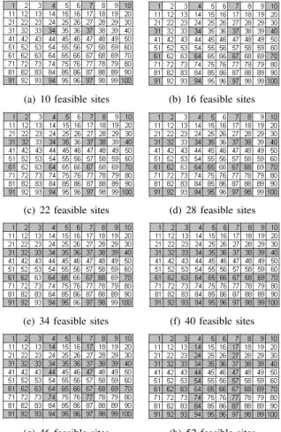
In the following, the sinks can move only on the feasible sites of Figure 5. Each node in the 10x10 grid is localized with its identifier number. The nodes in cells colored in gray are chosen as feasible sites.
We varied the number of feasible sites from 10 to 52 as shown in Figure 6. The number of sinks was fixed to 3, the number of sensors to 100 and the period sojourn time to 30 days. We notice that the network lifetime improves considerably when the number of feasible sites increases. In fact, the more the number of sites is, the more the sinks
(a) 10 feasible sites (b) 16 feasible sites
(c) 22 feasible sites (d) 28 feasible sites
(e) 34 feasible sites (f) 40 feasible sites
(g) 46 feasible sites (h) 52 feasible sites
Figure 5. The network with different number of feasible sites
Figure 6. The network lifetime with different number of feasible sites
to efficient locations move which leads to longer lifetime. Nevertheless, the choice of the feasible sites positions has a great influence on the network lifetime.
5.2. The Sinks Sojourn Times
We studied the pattern of the distribution of the sinks sojourn times at the different nodes. All the nodes of the grid can be feasible sites. Figures 7, 8, 9, 10, and 11 show the sojourn times of three sinks in 10x10 grid for respectively Static, Periphery, Random, Cluster and ILP schemes.
Figure 7. Sinks sojourn times at the different nodes of 10x10 grid network with Static scheme
Figure 8. Sinks sojourn times at the different nodes of 10x10 grid network with Periphery scheme
Figure 9. Sinks sojourn times at the different nodes of 10x10 grid network with Random scheme
The optimal sinks locations obtained for static sinks are the nodes which are almost at minimum distance i.e., number of hops to all other nodes. In Random scheme, the sinks sojourn time is variably distributed among all the nodes of the network. In the Periphery scheme, it is fairly distributed
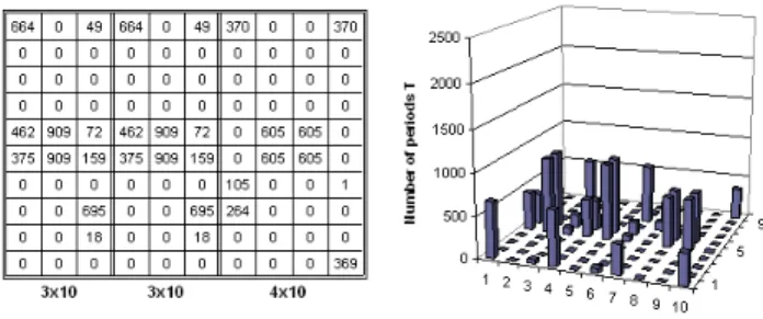
Figure 10. Sinks sojourn times at the different nodes of 10x10 grid network with Cluster scheme
Figure 11. Sinks sojourn times at the different nodes of 10x10 grid network with ILP scheme
among the nodes in the perimeter of the network. For the Cluster scheme, the grid 10x10 was divided in 3 clusters 3x10, 3x10 and 4x10 in which the sinks move separately. We notice that the sink sojourns most of the times at the corners and the central grid area of its cluster. In the ILP scheme where the sinks move in the entire network, the same pattern is obtained, the sinks sojourn most of the times at the corners and the central grid area as shown in Figure 11. Independently of the size of the network and the number of the sinks as shown in Figure 12 and 13, the optimal locations of the sinks according to ILP solution are the four corners of the grid, then the central grid area. The sojourn of the sinks at the central grid area can be explained as follows. If one of the sinks is located in the center of the grid it will have four neighbors within the transmission range. Contrarily, if it is located in the perimeter or the corner, it will have respectively three and two neighbors. Obviously, the more neighbors within the transmission range the sink has, the better the traffic load balanced among nodes is and the higher lifetime is. However, independently of where the sinks are located, the sensors in the corners drain less energy on forwarding packets than the sensors in the center which are always along a routing path to reach the sinks. For this reason, the sinks sojourn more at the nodes in the corners than the nodes in the central grid area in order to consume the residual energy of the ”rich” sensors.
Figure 12. ILP sinks sojourn times at the different nodes of 8x8 grid network
Figure 13. ILP sinks sojourn times at the different nodes of 9x9 grid network
5.3. The energy distribution
We analyzed the impact of the five schemes on the energy consumption at lifetime end in a network with 3 mobile sinks and 100 sensors. The distribution of energy consumption when the first sensor dies is depicted in Figures 14(a), 15(a), 17(a), 16(a) and 18(a). A light color means a higher percentage of energy consumption.
It is remarkable in all the figures that the energy consump-tion is highly variable and depends on the sinks locaconsump-tions. We notice that the nodes near the sinks have relatively higher energy consumption compared to most of the others because they have to receive and relay all other neighbors data in addition to their own data. This leads them to consume more energy.
In Figure 14(a), we observe that higher percentage of energy consumption is concentrated around three nodes in the grid which are the locations of the static sinks whereas the other sensors have a lower amount of energy consumption (dark color).
When the sinks move on the periphery of the network, the highest energy consumption occurs in nodes closest to the boundary of the network while the others nodes specially in the center consume less energy as seen in Figure 15(a).
In the Cluster scheme as shown in the Figure 16, the energy consumption is only balanced among the nodes of every cluster and not in the whole network. This is because of the restriction of sinks mobility to theirs clusters.
Figure 17(a) shows that Random scheme results in a better
(a) Energy consumption
(b) Residual energy
Figure 14. Static scheme in 10x10 grid network
(a) Energy consumption
(b) Residual energy
(a) Energy consumption
(b) Residual energy
Figure 16. Cluster scheme in 10x10 grid network
(a) Energy consumption
(b) Residual energy
Figure 17. Random scheme in 10x10 grid network
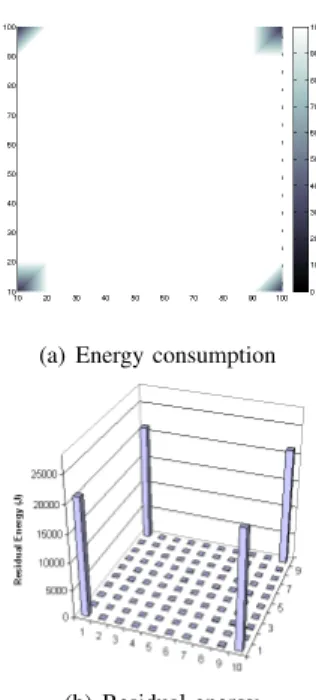
(a) Energy consumption
(b) Residual energy
Figure 18. ILP scheme in 10x10 grid network
balancing of energy consumption than Static, Periphery and Cluster schemes. In fact, we notice a larger area with light color.
However, ILP scheme balances almost perfectly the en-ergy consumption among the nodes. In fact, the majority of the nodes depleted their energy at the same time except the four corners as shown in Figure 18(a).
The distribution of the residual energy at each sensor node in 10x10 grid with 3 mobiles sinks was also studied (see Figures 14(b), 15(b), 17(b), 16(b) and 18(b)).
With static sinks, the majority of sensors have more residual energy at the end of network lifetime than the schemes with mobile sinks which have their initial energies more depleted at the lifetime end.
For the ILP scheme, sensor nodes have less residual energy than in the case of sinks moving in clusters. This is due to the fact that the mobility of sinks in the whole network changes the nodes acting as relays frequently and leads to balanced energy consumption among nodes. While, in the Cluster scheme, the movement of the sinks is restricted to their own clusters. So, this approach prevents to have global view of the entire network.
The ILP scheme results in a better distribution of residual energy among the nodes compared to Cluster, Periphery, Random and Static schemes. The results show that the percentages of the residual energy that remain unused at the network lifetime end for Static, Periphery, Random, Cluster and ILP schemes are respectively 71 %, 45 %, 31 %, 31 %, 3 %. Moreover, the number of sensors which have more than 50 % of their initial energies left at lifetime end is 80,
36, 20, 27 and 4 respectively for Static, Periphery, Random, Cluster and ILP schemes
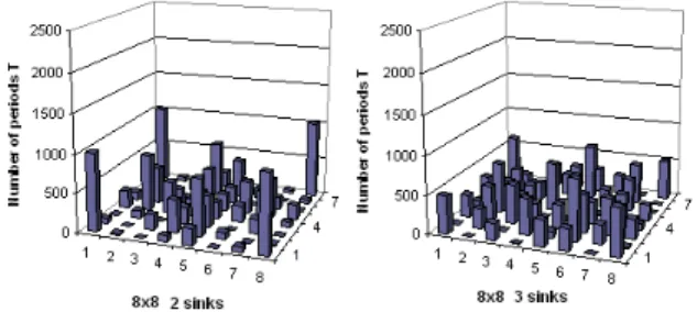
It is remarkable in the ILP scheme, as shown in the Figure 18(b), that the sensor nodes in the corners have higher energy at the end of network lifetime than the others nodes. This can be explained by the fact that they do not drain their energy in forwarding neighbor’s data in addition to their own data. Moreover, we observe that at the end of network lifetime the distribution of residual energy in the grid is more bal-anced among the nodes when the number of sinks increases (See Figure 19). The use of more sinks results in the reduction of the average path length between the sensors and sinks thus enabling to achieve less traffic load to the nodes and increased network lifetime.
(a) 2 sinks (b) 3 sinks
(c) 4 sinks
Figure 19. Residual energy distribution of ILP scheme in 5x5 grid network with increasing number of sinks
These results are interesting since they are not pure theory. We tried to approach realistic buildings deployment parameters in our assumptions and especially with sinks that can not move frequently.
6. Conclusion and future Work
In this paper, we have explored the problem of positioning multiple mobile sinks in wireless sensor networks inside buildings, in order to avoid the energy hole problem and extend the network lifetime, which is really needed in practice.
As a solution, we have proposed an ILP which directly maximizes the network lifetime instead of minimizing the energy consumption or maximizing the residual energy, which is what was done in previous solutions. The proposed ILP determines the best way to relocate sinks by giving their optimal locations and the duration of their sojourn time.
A comparative study of the proposed solution with static sinks, mobile sinks moving in the periphery of the network, mobile sinks moving randomly and mobile sinks moving separately in different clusters was made. Relocating sinks with our solution and using realistic parameters assumptions results in the sensor network lifetime extension and the energy consumption more balanced among the nodes. The lifetime improvements achieved in our experiments by de-ploying 3 mobile sinks in the network with hundred sensors are almost 99 % against 3 mobile sinks moving separately in different clusters and almost 230 % against 3 static sinks. The study of the pattern of the distribution of the sinks at different locations showed that the sinks sojourn most of times at the nodes in the central grid area and in the corners. This corresponds to very interesting feasible sites in buildings because the sinks can be easily relocated in the corridors which are often in the center of the buildings and provided with power and Internet access.
The weakness of the proposed approach is the scalability problem in networks with thousands of sensors due to the high ILP resolution complexity. In order to adopt this solution in a large scale wireless sensor network with more than hundreds of sensors, the network might be divided in several sensor sub-networks which will be deployed in the each part of the building. More than one sink can then be placed inside each zone to collect the information of the in-door environment. To implement the solution in a real environment and apply the model in real time conditions, technicians will be in charge of relocating the mobile sinks in the open areas of the buildings after long periods (i.e., months).
In our future work, we intend to improve the proposed ILP by including parameters and constraints that model more realistic requirements of an indoor environment (e.g., collisions) and take into account the energy consumption of sensing and data processing. We envisage also to introduce optimization in data routing by considering relevant metrics like latency, control overhead.
References
[1] L. Ben Saad and B. Tourancheau, “Multiple mobile sinks positioning in wireless sensor networks for buildings,” in
3 rd International Conference on Sensor Technologies and Applications SensorComm, 2009.
[2] J. Pan, Y. T. Hou, L. Cai, Y. Shi, and S. X. Shen, “Topology control for wireless sensor networks,” in Proceedings of the
9th annual international conference on Mobile computing and networking MobiCom, 2003, pp. 286–299.
[3] X. yang Li, W. zhan Song, and Y. Wang, “Topology control in heterogeneous wireless networks: Problems and solutions,” in Proceedings of the 23rd Joint Conference of the IEEE
[4] A. Sankar and Z. Liu, “Maximum lifetime routing in wireless ad-hoc networks,” in Proceedings of the 23rd Annual Joint
Conference of the IEEE Computer and Communications So-cieties INFOCOM, vol. 2, 2004, pp. 1089–1097.
[5] K. Fodor and A. Vid´acs, “Efficient routing to mobile sinks in wireless sensor networks,” in WICON ’07: Proceedings of
the 3rd international conference on Wireless internet. ICST,
Brussels, Belgium, Belgium: ICST (Institute for Computer Sciences, Social-Informatics and Telecommunications Engi-neering), 2007, pp. 1–7.
[6] O. Younis and S. Fahmy, “Distributed clustering in ad-hoc sensor networks: A hybrid, energy-efficient approach,” in
Proceedings of the 23rd Annual Joint Conference of the IEEE Computer and Communications Societies INFOCOM, 2004,
pp. 629–640.
[7] S. R. Gandham, M. Dawande, R. Prakash, and S. Venkatesan, “Energy efficient schemes for wireless sensor networks with multiple mobile base stations,” The IEEE Global
Telecommu-nications Conference GLOBECOM, 2003.
[8] W. Alsalih, S. Akl, and H. Hassanein, “Placement of multiple mobile base stations in wireless sensor networks,” IEEE
In-ternational Symposium on Signal Processing and Information Technology, 2007.
[9] X. Wu, G. Chen, and S. K. Das, “Avoiding energy holes in wireless sensor networks with nonuniform node distribution,”
IEEE Transactions on Parallel and Distributed Systems, 2008.
[10] ——, “On the energy hole problem of nonuniform node distribution in wireless sensor networks,” IEEE International
Conference on Mobile Adhoc and Sensor Systems MASS,
2006.
[11] J. Lian, K. Naik, and G. B. Agnew, “Data capacity improve-ment of wireless sensor networks using non-uniform sensor distribution,” in International Journal of Distributed Sensor
Networks, 2005.
[12] A. Bogdanov, E. Maneva, and S. Riesenfeld, “Power-aware base station positioning for sensor networks,” in Proceedings
of the IEEE INFOCOM, 2004, pp. 575–585.
[13] E. Oyman and C. Ersoy, “Multiple sink network design problem in large scale wireless sensor networks,” IEEE
In-ternational Conference on Communications, 2004.
[14] H. Kim, Y. Seok, N. Choi, Y. Choi, and T. Kwon, “Optimal multi-sink positioning and energy-efficient routing in wireless sensor networks,” Lecture Notes in Computer Science LNCS, 2005.
[15] J. Luo and J.-P. Hubaux, “Joint mobility and routing for life-time elongation in wireless sensor networks,” In Proceedings
24th Annual Joint Conference of the IEEE Computer and Communications Societies INFOCOM., 2005.
[16] K. Akkaya and M. Younis, “Sink repositioning for enhanced performance in wireless sensor networks,” Elsevier Computer
Networks Journal, 2005.
[17] B. Wang, D. Xie, C. Chen, J. Ma, and S. Cheng, “Employing mobile sink in event-driven wireless sensor networks,” IEEE
Vehicular Technology Conference VTC, 2008.
[18] Z. M. Wang, S. Basagni, E. Melachrinoudis, and C. Petrioli, “Exploiting sink mobility for maximizing sensor networks lifetime,” In Proceedings of the 38th Annual Hawaii
Inter-national Conference on System Sciences HICSS, 2005.
[19] S. Basagni, A. Carosi, E. Melachrinoudis, C. Petrioli, and Z. M. Wang, “Controlled sink mobility for prolonging wire-less sensor networks lifetime,” Wirewire-less Networks, 2007. [20] Y. Bi, J. Niu, L. Sun, W. Huangfu, and Y. Sun,
“Mov-ing schemes for mobile sinks in wireless sensor networks,”
Performance, Computing, and Communications Conference,
2007.
[21] R. C. Shah, S. Roy, S. Jain, and W. Brunette, “Data mules: Modeling a three-tier architecture for sparse sensor networks,” in IEEE International Workshop on Sensor Network Protocols
and Applications SNPA, 2003, pp. 30–41.
[22] M. Marta and M. Cardei, “Improved sensor network lifetime with multiple mobile sinks,” Pervasive and Mobile computing, 2009.
[23] Z. Vincze, R. Vida, and A. Vidacs, “Deploying multiple sinks in multi-hop wireless sensor networks,” IEEE International
Conference on Pervasive Services, 2007.
[24] A. Azad and A. Chockalingam, “Mobile base stations place-ment and energy aware routing in wireless sensor networks,”
IEEE Wireless Communications and Networking Conference WCNC, 2006.
[25] D. Maniezzo, K. Yao, and G. Mazzini, “Energetic trade-off between computing and communication resource in multi-media surveillance sensor network,” 4th IEEE Conference
on Mobile and Wireless Communications Networks MWCN,
2002.
[26] CPLEX http://www.ilog.fr/products/cplex/.
[27] Chipcon. CC2420 2.4 GHZIEEE 802.15.4 / ZigBee-ready