Phoresis in turbulent flows

HAL Id: hal-02633847

https://hal.archives-ouvertes.fr/hal-02633847

Submitted on 27 May 2020

HAL is a multi-disciplinary open access

archive for the deposit and dissemination of

sci-entific research documents, whether they are

pub-lished or not. The documents may come from

teaching and research institutions in France or

abroad, or from public or private research centers.

L’archive ouverte pluridisciplinaire HAL, est

destinée au dépôt et à la diffusion de documents

scientifiques de niveau recherche, publiés ou non,

émanant des établissements d’enseignement et de

recherche français ou étrangers, des laboratoires

publics ou privés.

Phoresis in turbulent flows

Vishwanath Shukla, Romain Volk, Mickaël Bourgoin, Alain Pumir

To cite this version:

Vishwanath Shukla, Romain Volk, Mickaël Bourgoin, Alain Pumir. Phoresis in turbulent flows. New

Journal of Physics, Institute of Physics: Open Access Journals, 2017, 19, �10.1088/1367-2630/aa99bd�.

�hal-02633847�

PAPER • OPEN ACCESS

Phoresis in turbulent flows

To cite this article: Vishwanath Shukla et al 2017 New J. Phys. 19 123030

View the article online for updates and enhancements.

Related content

Osmotic manipulation of particles for microfluidic applications

B Abécassis, C Cottin-Bizonne, C Ybert et al.

-Phenomenology of buoyancy-driven turbulence: recent results

Mahendra K Verma, Abhishek Kumar and Ambrish Pandey

-MODELING THE POLLUTION OF PRISTINE GAS IN THE EARLY UNIVERSE

Liubin Pan, Evan Scannapieco and Jon Scalo

New J. Phys. 19(2017) 123030 https://doi.org/10.1088/1367-2630/aa99bd

PAPER

Phoresis in turbulent flows

Vishwanath Shukla1,2_{, Romain Volk}1_{, Mickaël Bourgoin}1_{and Alain Pumir}1,3

1 _{Univ Lyon, ENS de Lyon, Univ Claude Bernard, CNRS, Laboratoire de Physique, F-69342 Lyon, France} 2 _{Service de Physique de l’Etat Condensé, Université Paris-Saclay, CEA Saclay, F-91191 Gif-sur-Yvette, France} 3 _{Author to whom any correspondence should be addressed.}

E-mail:[email protected],[email protected],[email protected]@ens-lyon.fr

Keywords: turbulence, phoresis, direct numerical simulations, turbulent transport

Abstract

Phoresis, the drift of particles induced by scalar gradients in a

flow, can result in an effective

compressibility, bringing together or repelling particles from each other. Here, we ask whether this

effect can affect the transport of particles in a turbulent

flow. To this end, we study how the dispersion

of a cloud of phoretic particles is modified when injected in the flow, together with a blob of scalar,

whose effect is to transiently bring particles together, or push them away from the center of the blob.

The resulting phoretic effect can be quantified by a single dimensionless number. Phenomenological

considerations lead to simple predictions for the mean separation between particles, which are

consistent with results of direct numerical simulations. Using the numerical results presented here, as

well as those from previous studies, we discuss quantitatively the experimental consequences of this

work and the possible impact of such phoretic mechanisms in natural systems.

1. Introduction

The transport of particles and macro-molecules in aflow can be strongly affected by a scalar quantity present in thefluid. The phenomenon of phoresis investigated here results from a drift velocity of the particles, vd,

proportional to the gradient of a scalar quantity,q (x,t):vd=  (a q x, t). The scalarfield involved could be

temperature(thermophoresis), a chemical species (chemophoresis), or salt concentration (diffusiophoresis). The magnitude and sign of the phoretic mobility coefficient α depends on the nature of the interaction of the particle with the scalarfield [1]. Electrophoresis and magnetophoresis [2,3], induced by a drift proportional to

the electric or magneticfield, respectively, provide two extra examples of phoresis with potential practical utility. It is well-known that the diffusive transport of particles and of macro-molecules in a laminarflow is

generally very slow because of their very small intrinsic molecular diffusion coefficient. Recent studies show that a significant enhancement of the transport properties can be achieved by addition of a small salt concentration to the solution, which induces a phoretic mobility in response to the salt gradients[4,5]. The enhanced mobility of

the colloids observed in microfluidic channel experiments with salt gradients [4,5] was initially interpreted in

terms of an effective diffusion aided by diffusiophoresis. The inferred diffusion coefficient is larger than what is expected from a simple Brownian motion of colloidal particles and for certain salts it is almost two orders of magnitude larger. This makes diffusiophoresis an important concept with a practical utility, which can be used to selectively control the mobility of colloids or macro-molecules in microfluidic devices for scientific and/or industrial purposes. Similar arguments based on effective diffusivity were later used to explain the experimental results on enhanced or delayed mixing of colloids in chaoticflows [6].

However, more recent studies[7,8] showed that a description of these phenomena in terms of a modulated

diffusion coefficient does not capture all the physics at play. In particular, it fails to explain the evolution in space and time of the colloids concentration, especially mixing and de-mixing at short times.

These studies stressed the importance of the effective compressibility of the velocityfieldvseen by the particles:·v¹0. Numerical simulations and experiments employing diffusiophoresis in chaoticflows have conclusively shown that the compressibility strongly affects the transport of particles. In particular, it was found that the compressible nature of the velocityfield acts as a source of colloids concentration variance [7]. As a

OPEN ACCESS

RECEIVED

18 September 2017

REVISED

8 November 2017

ACCEPTED FOR PUBLICATION

10 November 2017

PUBLISHED

12 December 2017

Original content from this work may be used under the terms of theCreative Commons Attribution 3.0 licence.

Any further distribution of this work must maintain attribution to the author(s) and the title of the work, journal citation and DOI.

consequence the whole mixing process is modified by the phoretic transport, leading to either mixing or de-mixing depending on the local environment. Moreover recent experiments in a chaoticflow clearly

demonstrated that diffusiophoresis modifies the properties of the particle distribution not only at small-scales, but even at the largest scales of the mixing process[8].

Here, we ask how the transport of colloids by a turbulentflow is affected by phoresis. Turbulent motion in fluids involves a wide range of length and time scales and is known to enhance mixing by generating strong gradients of advected scalarfields. The study of the transport of particulate matter in turbulent flows is an important problem, with far reaching implications for a wide spectrum of applications, such as rain initiation in warm clouds[9] or controlling industrial flows [10]. The velocity field experienced by inertial particles, with a

finite-size and/or different density compared to the carrier fluid, is compressible [11,12]. It is known that this

effective compressibility results in an inhomogeneous distribution of inertial particles[13–15] in contrast to the

homogeneous distribution of pure tracer particles in turbulentflows. Therefore, it is natural to use the concepts and current understandings of the role played by the effective compressibility in turbulent transport processes, when extended to phoretic particles driven by turbulent scalarfield [16–19].

In the following, we examine the consequences of the turbulentfluctuations on the dynamics of a cloud of particles undergoing phoresis. In the spirit of the original experiments, documenting phoretic effects by injecting locally colloids and salt[4,5], we focus on the effect of phoretic compressibility at short times, after

releasing a cloud of salt and colloids, of characteristic sizeℓc, in a turbulentflow. Although it is transported by a

turbulentflow, such a cloud of size ℓcwill grow ballistically during a characteristic time tc, which can be

estimated using the standard phenomenological description of turbulence(see section3, and[20]).

Dimensionally, the effective compressibility( · ), wherev vis the velocity seen by the particles, is an inverse time scale, which should be compared to the typical time scale of the motion; note thatvincludes both the velocity of the carrierflow u and the phoretic drift vd. Therefore, we introduce a dimensionless number,

t

v c



F ~ ( · )´ , which characterizes the competition between turbulent dispersion and compressibility. We

use these phenomenological arguments, which are corroborated by direct numerical simulations(DNS) of the Navier–Stokes equations (NSE), to show thatFis the parameter which controls the mixing of the phoretic

particles in this problem. In particular, we show that the maximum contraction of the particle cloud occurs in the ballistic regime of turbulent dispersion, and varies as exp(- Fg ). Our results show thatγ has similar values

for different Reynolds numbers and particle cloud sizes, thereby suggesting an universal behavior.

Phoretic effects have also been observed to play a role in randomly stirred chaoticflows in two dimensions [7], in a regime where the scalar field is in a statistically stationary state. We discuss the expression ofFin such

cases. Our estimates, obtained by using realistic values of the physical parameters, suggest that phoretic effects should also be observable in turbulentflows in steady state configuration at very small scales.

2. Methods

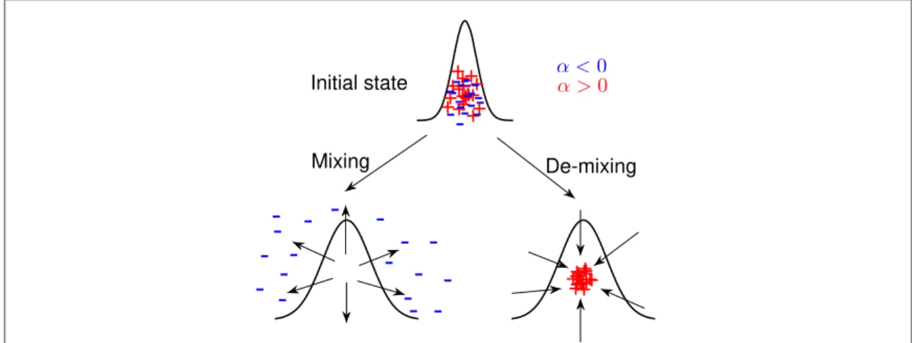
Specifically, we consider here a simple problem, whereby a blob of scalar field with a simple Gaussian profile is released in a turbulentfluid, along with a cloud of particles, as illustrated in figure1. The scalarfield decays, as it is mixed by the turbulence. During this process, strong scalar gradients develop and this drives the phoretic motion of the particles. We stress that this configuration is experimentally realizable, for example in a turbulent jet or a water-tunnel, where the statistical properties of the cloud of particles and their dispersion could be accurately measured. We assume here that theflow is incompressible, so that its description is based on the (NSE)

t p

u

u u _n 2u f, 1

¶

¶ +( ·) = - +  + ( )

where ·u=0imposes the incompressibility condition on the three-dimensional(3D) velocity field u. p is the pressurefield, ν is the fluid viscosity andfis the forcing term, acting at large scales, which maintains the turbulent flow statistically stationary. In equation (1), we have, without any loss of generality, set the density of the fluid to 1. The

spatio-temporal evolution of the scalarfield fluctuationsq (x,t)is governed by the advection-diffusion equation

t u , 2 2 q q k q ¶ ¶ +( ·) =  ( )

whereκ is the diffusion coefficient of the scalar field constituents, whose spatial averageá ñqspatialis zero. We

furthermore assume that the molecular diffusion coefficient of the colloidal particles of interest here is orders of magnitude smaller than the constituents of the scalarfield. Therefore, we are interested in the limiting case where the particles are advected by the combined velocityfield of the turbulent flow u and the phoretic contribution vd=  ,a q α being the phoretic mobility coefficient, quantifying the efficiency of the gradient to

generate an additional drift motion for the particles. To study the dynamics of this assembly of discrete particles undergoing phoresis in a turbulent environment, we adopt a Lagrangian framework, in which the velocity of a

particle, labeled by the index i, and located at positionXi( )t is given by

t t

vi=u X( i, )+ a q(Xi, ), ( )3 wheredXi dt= .vi

As briefly sketched in the previous section, the phenomenological approach of particle dynamics used here is

based on the standard(Kolmogorov–Obukhov) phenomenological description of turbulence [20]. A 3D

turbulentflow is sustained by injecting energy at a rate ε per unit mass, at the large length scales, ℓ∼L0,

comparable to the system size. This energy is transferred to smaller length scales, down to the scaleη where

energy is dissipated by viscosity:_{h= (n e}3 ₎1 4_{. The range of scales, defined by L}

0

h ℓ , is defined as the

inertial scales. The transfer of energy is a result of the nonlinear interactions, represented by the advection term in the NSE(1). An (almost) self-similar structure is often postulated over the inertial range of scales, which is

characterized by a constantflux of energy, ε [20].

We test our phenomenological arguments and make them more quantitative by numerically determining the statistical properties of this system. To this end, we perform DNSs of the NSE(1) and the advection-diffusion

equations(2) in 3D to determine the fluid velocity field u and the scalar field θ, respectively; we then use them to

numerically determine the trajectories of the particles. We solve the NSE in a triply-periodic domain by using the pseudospectral code, as described, e.g. in[15,21]. The flow is maintained statistically stationary by forcing the

velocityfield at large scales (small wave numbers k) [21]. Simulations were carried out at moderate resolutions,

with 963, 1923and 3843Fourier modes. Adequate spatial resolution for the velocityfield was imposed, by maintaining the product kmaxh 1.5. This allowed us to simulateflows up to a Taylor-scale Reynolds number

Rl=175. To address the more demanding resolution criteria for the scalarfield [21], we work here with a dimensionless ratio n k equal to 1/2. We refer here to this dimensionless ratio as the Prandtl number Pr, a terminology which is generally used when for a scalarfield (the corresponding dimensionless ratio is known as the Schmidt number, Sc, in the case of a concentrationfield).

Here, we start with an initial configuration, where we release in a turbulent flow a Gaussian blob of scalar:

t x, 0 exp x 2 _c 4 0 2 2 q = =q ⎛ -⎝ ⎜ ⎞ ⎠ ⎟ ℓ ( ) ( )

containing 2000 particles which are randomly distributed within it with the same Gaussian distribution. The size ℓcthen serves as a convenient measure both of the scalar blob and the particle cloud. The effect of the scalar is to

attract particles close to the center whenaq > , and repel them away from the center when0 0 aq < , as0 0

illustrated infigure1.

A list of the simulations carried out in this work is provided in tablesA1andA2, seeappendix.

3. Results

3.1. Competition between phoretic effects and turbulence mixing

As already stressed, the velocityfield seen by the particles, (3), is compressible and its divergence is proportional

to the Laplacian of the scalarfield_{ ·}v _{= a} 2_{q. The divergencefield(x,t)º ·vcan serve as a local}

Figure 1. Turbulent phoresis. Schematic diagram showing the initial configuration of the scalar field and the resulting phoretic motion of the colloids. Particles with positive₍a >0, red_{‘+’ symbol) and negative (}a <0, blue_{‘–’ symbol) phoretic mobilities are initially} distributed in a Gaussian blob of scalarfield (upper narrow Gaussian profile). Scalar mixing in a turbulent fluid is indicated by drawing a broader scalar profile; depending on the sign of the phoretic mobility α, the particles either tend to cluster (de-mixing) or separate from each other(mixing).

3

indicator of the compressibility. With(4) as the initial condition for the scalar field, the initial compressibility is

given by0~aq0 ℓ_c2. Starting from initial condition, the blob offluid which contains both scalar and particles

will be advected by turbulent motions. Particles will then experience compressible effects at the scaleℓc(of the

order0), until the scalar field is distorted, which is achieved in a time tccorresponding to the eddy turnover

time at scaleℓc. Such a time scale can be estimated following standard phenomenology of turbulentflows [20].

Asℓclies in the inertial range, tcdoes not depend on the viscosity and reads tc~ ℓ( c2 e)1 3, whereε is the energy

injected per unit mass. This leads us to define the dimensionless parameter that characterizes the competition between turbulent dispersion and compressibility effects at a given scaleℓcby:

t . 5 c c 0 2  aq F = ℓ ( )

We chose to defineF > 0for the attracting case which corresponds toaq > , and0 0 fixedq = in all our0 1

DNS runs. Note that tcis Kolmogorov–Obukhov phenomenological estimate of the time for which an eddy of

the size of the scalar blobℓcsurvives in a turbulentflow.

3.2. Mixing and de-mixing of a turbulent cloud

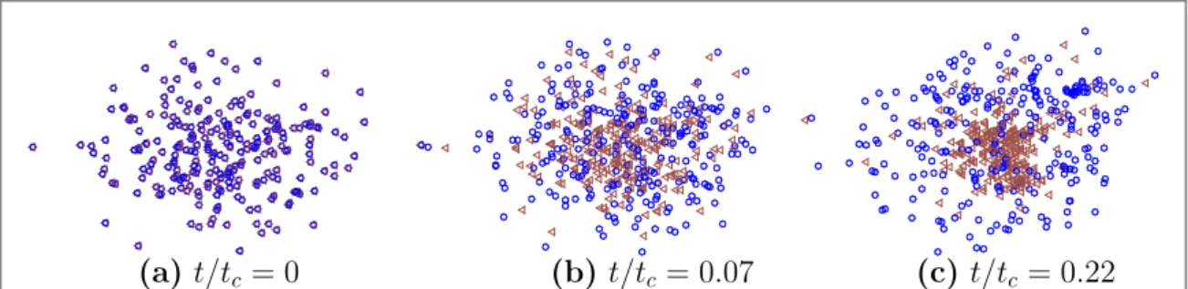
Infigure2we show the positions of two particle types at three different times:(a) t tc= ,0 (b) t tc=0.07, and (c) t tc=0.22. These two particle types correspond to two different values ofF = 5.81(brown triangles,

0

a > ) andF = - 5.81(blue circles,a <0). Starting at identical initial positions at t=0 (left), we observe that forF > 0(brown triangles,a >0) the particle cloud shrinks as a whole, whereas forF < 0(blue circles,

0

a < ) the particles in the cloud move away from each other, resulting in an overall expansion.

To quantify the coherent expansion or the contraction of the particle cloud at short times, we measure the mean relative separation between the particles r(t) and its ratio to its value at t=0

t r t r t 0 , 6 2 2  º = ( ) ( ) ( ) ( )

where r t2( )= á(Xi( )t -Xj( ))t 2ñ1i j N< . In order to get better statistics, 8 blobs of scalar containing particles are

released at the same time with distances larger than half the box size. The simulation is then run and stopped before the different deformed blobs overlap. Infigure3(a) we show the temporal evolution offorfive different values of



F for the DNS run for whichℓc h =20.8and Rl=95. The pink curve with squares represents the case of a pure tracerF = 0( =0 0). For the phoretic particles withF < 0(blue curves with circles and black curves with stars)

increases faster than it does for the pure tracers. This represents a case where the local environment selectively assists in the faster dispersal of these particles, thereby resulting in an enhanced mixing or expansion of the particle cloud at short times. In a direct contrast to this, for phoretic particles withF > 0(yellow curve with diamonds and

brown curve with triangles),first decreases until it reaches a minimum value and then it rises rapidly. This clearly represents a case of de-mixing aided by the local environment, whose extent depends on the value ofFand has been

quantified in terms of the coherent contraction of the particle cloud monitored by measuring.

In the following, we focus on the caseF > 0, which results in de-mixing(see figure3). We note that the

lower the value reached by, the stronger is the de-mixing. We propose here a simple description of this effect, based on the standard Kolmogorov–Obukhov phenomenological theory of turbulence [20], resulting in a

prediction ofminas a function ofF.

We can use(3) and (4) to write

t X u d d , 7 d d ad q = +  ( )

Figure 2. Mixing/de-mixing of phoretic particles. Positions of two particle types at three different times:t tc=0(a), t tc=0.07(b),

and t tc=0.22(c). The particles correspond to two different values of the dimensionless numberF = - 5.81(blue circles) and 5.81



F = (brown triangles) to same local environment, from the DNS run with Rl=95andℓc h =20.8. The particles withF > 0 de-mix, whereas the ones withF < 0undergo enhanced mixing, for a scalar blob with the Gaussian profile in a turbulent flow.

where Xd (resp.du) is the difference between the positions (resp. velocities) of two phoretic particles (indices i j, have been dropped for the sake of simplicity). Note that the first term on the right hand side in (7) is a velocity

increment. In the absence of phoretic effect(a =0), the termduis responsible for turbulent particle dispersion. This term averages to zero when the colloids are released, as the particle positions are a priori not correlated with the flow velocity field [22]. At small times, this term contributes only a small correction to the constant term, in particular

when∣F∣1, seefigure3. The second term is the phoretic contribution which produces the effect shown in figures2and3. At a qualitative level, this term is smooth and nearly isotropic so that one has(t< , Xtc d ~dX0)

t X X d d _c , 8 2 0 2 2 d aq d á ñ µ - á ñ ℓ ( )

when averaging over particle pairs in the ballistic regime of turbulent dispersion. As long as the injected blob of scalar keeps its identity(with a simple, connected shape, before being torn apart by the turbulent flow), the compression experienced by the set of particles leads to the overall contraction of the cloud, given by:

r r t t 2 ln c . 9 c 0 µ -F ⎛ ⎝ ⎜ ⎞_⎠⎟ ( )

The scalar blob retains its identity for a time»tc, so the particle cloud keeps contracting for a time»tc. During

this time interval, the value ofcontracts by an amount, which increases withF . Equationc (9) suggests a simple

relation betweenminandF:

exp c , 10

min 0

 ~ (- Fg ) ( )

whereγ is a constant a priori of order 1. We emphasize that this prediction results from the competition between the contraction introduced by the scalar, and the mixing by the turbulentflow.

We now turn to DNS runs to test the validity of this phenomenological prediction. Infigure3(b) we plotmin

versusFon log-linear scale for different particle cloud sizes and Reynolds numbers. We observe that for all the cases min

 decreases exponentially with increasingF, as confirmed by straight lines on log-linear axes and whose slopes γ

agree with each other within 15%. The inset offigure3(b) shows the plot oftmin tcversusFfor the cases considered

above. We notice that the time it takes to achieve maximum contraction of the particle cloud or the maximally de-mixed state for the phoretic particles has a tendency to saturate asFincreases. Moreover, wefind that the particle

cloud survives only for a fraction of time tc. Our error bars are large, indicating a need for better statistical averaging;

however, we believe that our conclusions will not change qualitatively.

As stressed in the introduction, the effect of phoresis on the transport properties of the particles can be best understood in terms of an effective compressibility. One way to characterize this compressibility, appropriate in the context of pair dispersion, is to introduce the dilation factor:

r r t t 1 d d 1 d d . 11 2 2   c = = ( )

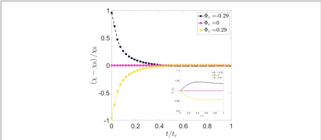
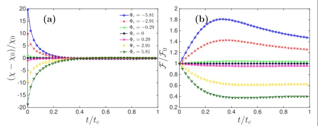
Figure4shows the dilation factorχ estimated for the smallest values ofFrepresented infigure3; as it was difficult to

see any measurable effect of phoresis in the latter. Figure4indicates that for values ofF » 0.3, the difference

Figure 3. Quantifying the de-mixing._{(a)Temporal evolutionof the ratio ofmean relative separationto its value att=0,}( )t º

r t2_{( )} r t2_{( =}0_{), for different values of the dimensionless numberF characterizing the effective compressibility, from the DNS run with} Rl=95andℓc h =20.8;tcis the time scale for which an eddy of sizeℓcsurvives in a turbulentflow. (b) Log-linear plotsof minimum of

versusF . minis representative of the maximal de-mixing attained. Inset: plots oftminversusF , shows that the time to achieve maximum de-mixing(or contraction of the particle cloud) initially increases and thensaturates at large values ofF .

5

betweenχ and the corresponding value in the case of a passive tracer,c , signi₀ ficantly deviates from 0. For completeness, the values ofχ for all the values ofFinfigure3are shown infigureA1, seeappendix. It can be seen

that even for values of _ 10 1



F = ₍ -_{)the impact of phoresis on the initial dilation factor is of order one compared to}

the non-phoretic situation. The inset offigure4, representing the ratio  then shows that although the dilation0

factor relaxes to the non-phoretic value in a timescale of a fraction of tc, a sustained modification of the mean square

pair separation of the order of 5% compared to the non-phoretic case does persist at timescales t» . It can also betc

noted that these alternative ways of presenting the data better emphasize the symmetry between the compressing situation(F > , showing a minimum ofc 0   , which was discussed earlier0 ) and the dilating situation (F <c 0),

showing an equivalent maximum of  . Thus, a value of0 F of order 10c −1is sufficient to affect the rate of dilation

of pairs of particles by a significant amount, albeit over a short time lapse. Yet, as suggested below, these effects may be prevalent in conditions where the scalar and the particles are in a steady state.

3.3. Short time separation of the particles in the cloud

To further understand the mixing and de-mixing process, we look at the two-particle statistics, where we compute how the relative separation between the particles changes with time. We again turn to

phenomenological arguments to predict the behavior of the mean-squared relative displacement at short-times

t t t t t X X v u 0 1 . 12 c c 2 2 2 2 2 2 2 2 2 2 2  d d d d a d q b á - ñ á ñ á ñ + á  ñ + F   ℓ ∣ ( ) ( )∣ ( ) [ ( ) ( ( )) ] ( ) ( )

In going from thefirst to the second line in the above equation, we have neglected the cross term uád ·d( ñq). This is justified by the complete lack of correlation between the injected scalar field θ and the flow velocity u. The dimensionless parameterβ introduced in equation (12), is expected to be independent of ℓcandRel. Therefore,

we can write t A t t X X 0 2 _c2 _c 2, 13 d d á∣ ( )- ( )∣ ñ ℓ = [ ¢] ( ) with t_c t 1c 2 1 2  b

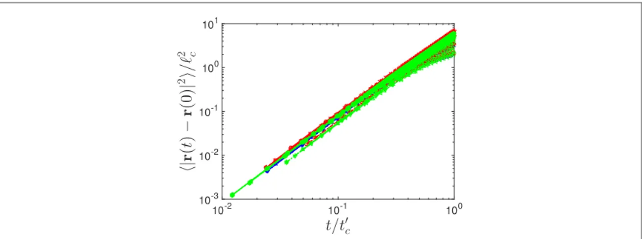
¢ = ₍ + F ₎- _{and A is a constant. Infigure5we show the log–log plots of mean-squared relative}

displacement_ádX t _-dX 0 2_{ñ ℓc}2

∣ ( ) ( )∣ versus scaled timet t_c¢for different values ofF(indicated by different

symbols) for three different Reynolds numbers Rel = 58(blue lines), Rel = 95(red lines), and Rel = 175

(green lines); and for different particle cloud sizes, see the caption of figure5, as well as tablesA1andA2in

appendixfor further details. These DNS runs confirm the phenomenological prediction that, when rescaled by the cloud sizeℓc, the mean-squared relative displacement is a linear function of(t tc¢)2in the ballistic regime.

Moreover, wefind that this statistical property is universal, as the plots for differentF,Relandℓccollapse onto

each forb 0.05.

We end this section with a remark that in the present study we are interested in an elementary question, whether phoretic effects can lead to measurable consequences. For this reason, we focus on a simple quantity,

Figure 4. Dilatation factor

t

1 d d 



c = and in the inset: mean square separation in presence of phoresis normalized by the non-phoretic case; from the DNS run with Rl=95andℓc h =20.8.

namely the mean-square separation. However, much insight can be gained by systematically investigating the full distribution of separation at different times. Such an investigation will be the subject of future work.

4. Discussion of the orders of magnitude: are phoretic effects observable?

Whether phoretic effects(thermo- and diffusio-phoresis, in particular) can give rise to measurable effects is the important question that we address now. The present discussion is based on the parameterF , introduced inc (5),

which has been demonstrated in simple problems, see section3, to provide a good way to quantify the importance of phoretic phenomena: the largerFthe larger the effect of phoresis.

4.1. Revisiting the definition ofF

In terms of possible applications, two effects need to be taken into account when defining the parameterF,

relevant to evaluate the importance of phoretic effects.

First, the phoretic coefficient α is generally found to depend on the local scalar field θ, with a dependence of the forma=Dp q, where Dphas the dimension of a diffusion coefficient [4,5,23]. This implies that the

dimensionless expression of theflow compressibility, equation (5) simplifies to:

Dpt , 14 c lim 2  F = ℓ ( )

whereℓcis the small length scale of the scalarθ ( µ2q q ℓc2), and tlimis the persistence time of thefluctuations

ofθ inducing phoresis. In our problem, turbulence disrupts a blob of scalar of size ℓc, in a time tlimthat depends

on theℓc.

Second, whereas in studying phoretic effects in section3, we have explicitly considered scalars with a diffusion coefficient of the order of viscosity: Pr» , it should be kept in mind that in practice, the diffusion1 coefficient of the scalar can be significantly smaller than viscosity:Pr »6in the case of thermophoresis, and Pr≈1000 in the case of diffusiophoresis. We begin this section by discussing the parameterFby taking into

account the expressiona=Dp q, and the large values of Pr.

The following discussion rests on the classical picture of the mixing of a scalarfield by a turbulent flow. The fluctuations of the velocity field typically extend over a range of length scales, from the large (stirring) length, L, down to the Kolmogorov scale,η. A scalar field, advected by the flow, is also subject to molecular diffusion,

Pr

kºn , where Pr is the Prandtl number already introduced. In applications with large Prandtl number the scalarfluctuations can extend down to scales much smaller than η. In fact, the smallest scale of the scalar fluctuations,h , known as the Batchelor scale, is of orderB hBºhPr-1 2for Pr1[24].

The persistence of scalarfluctuations at a scale ℓcdepends on the range of scale. Namely, whenhℓcL

(the size of the scalar blob lies in the inertial range), the blob is subject to the turbulent shear,µ(e ℓc2 1 3) , so the

persistent time is tlimµ ℓ( _c2 e)1 3. This is the case we have considered so far. In this case, the expression(14)

reduces to

Figure 5. Ballistic mean squared relative displacement at short times loglog plots of the mean-squared relative displacement t

X X 0 2 c2

d d

á∣ ( )- ( )∣ñ ℓ versus scaled timet tc¢, where tc t 1c 2

1 2

 b

¢ = ₍ + F ₎- _{, obtained from DNS runs for different values ofF} (represented by different symbols) for three different values of Taylor-microscale Reynolds numberRel = 58(blue dashed lines

10.7 c h =

ℓ ), 95 (red lines: dashedℓc h =20.8and colon(:)ℓc h =12.0) and 175 (green lines: dashedℓc h =50.5, colon(:) 30.3

c h =

ℓ and dashed-dotℓc h =10.1); different values of particle cloud size ℓcis indicated by different line-types. In our

simulationsD =q 1and tcis time scale associated withℓc. See tableA2for more details.

7

D 15 p c 4 3  n h F = ⎛ ⎝ ⎜ ⎞ ⎠ ⎟ ℓ ( )

which immediately shows that the largest possible value ofFis obtained whenℓc»h:F Dp n. In the other

regime,hBℓch, the velocityfield is smooth at the scale ℓc, and the strain acting on a blob of sizeℓcis

1 2

e n

µ( ) . This implies that the time tlimµ (n e)1 2, which is also known as the Kolmogorov time scale[20]. In

this case, the expression forFreduces to:

D D D . 16 p c p c p c 2 1 2 2 B 2  n e n h k h F = ´⎜⎛ ⎟ = ´ = ´ ⎝ ⎞⎠ ⎛ ⎝ ⎜ ⎞ ⎠ ⎟ ⎛ ⎝ ⎜ ⎞ ⎠ ⎟ ℓ ℓ ℓ ( )

Equation(16) shows that the value ofFcan vastly exceed Dp n, the limiting value whenℓc h. Specifically, in

the case of blobs of sizeℓc»hB,F » Dp k. These expressions are particularly relevant, given the large values

of Pr in the relevant cases of thermo- and diffusiophoresis.

To summarize, the estimates given so far show that the maximum strength of the phoresis effects quantified in terms of the parameterFcan be ultimately expressed as ratio of the diffusion coefficient Dpand either the

viscosityν or the diffusion coefficient of the scalar field (temperature or salt) κ. 4.2. How large are phoretic effects?

To proceed, we use the values of Dpreported in the literature. Microfluidic experiments have shown so far a

maximum effect when using carboxylate colloids in gradients of lithium chloride(LiCl), this combination of particle and salt lead to a diffusiophoretic coefficient as large as Dp≈300 μm2s−1. In experiments on

thermophoresis values of Dpas large as 3000μm2s−1have been measured[23], hence 10 times larger than in the

diffusiophoresis case. These estimates are consistent with those measured in the oceans[25].

This implies that the ratio Dp n, which corresponds to the largest possible value ofFwhenℓcis in the

inertial range, see(15), is of the order 10−4in the case of diffusiophoresis, and of order 3_´10-3_{in the case of}

thermophoresis.

These values are clearly smaller than the values necessary to measure any of the effects discussed in section3. Assuming, however, a value ofℓcsmaller thanη, but larger thanh shows that the values ofB Fcannot be larger

thanF 0.02in the case of thermophoresis, andF 0.1in the case of diffusiophoresis. These values are

sufficient to observe, in principle, a significant effect of diffusiophoresis.

It is useful to compare the previous estimates with existing experimental results, where effects of phoresis were unambiguously found.

In the microfluidic experiments on diffusiophoresis by Abecassis et al [4,5], using a laminar flow, the

limiting time is given by the mean advection tlim=zobs U0(where zobsis the observation position along the

micro-channel and U0is the advection velocity along the channel). Interestingly,Fin their experiment can

then be estimated to be in the range 10_[ -3_–10-1_{], with measurable effects on the spreading and focusing of the}

concentration profile of an initial colloidal band.

For the experiments in chaoticflows by Desseigne et al [6] and Mauger et al [8], which are closer in spirit to

the present work, the limiting time scale at the early stage of the process is given by the period of the chaotic cycle (at larger times the diffusion time of salt also becomes important), leading to typical values ofFof the order of

10-3 10-2

[ – ], with subtle but still measurable effects on the concentrationfield of colloids and its gradients. We also notice that Schmidt et al[17] report a possible observation of diffusiophoresis, by looking at clustering

properties of particles at inertial scales in a turbulent gravityflow with salt gradients. In such conditions, the largest expected value forFis of the order of Dp n(with ν the kinematic viscosity of the fluid), which in their

experiment is of the order of 10−4.

It is worth pointing out that in the problem of pair dispersion, as we have studied it numerically, the initial scalar distribution affects colloid transport for a small time only. Scalar gradients, in a statistically steady-state regime, may act cumulatively, resulting in much larger effects. As such, the requirement in term ofFto observe

a significant phoretic effect could be conceivably much reduced, compared to what we found in the purely transient problem investigated here.

The above discussion and the values ofFobtained on the basis of[23,25] indicate that the phoretic effects

can be important and therefore may affect the transport of small organisms, or pollutant particles, as a result of local gradients of salinity, dissolved oxygen, temperature, etc.

5. Summary

In this work, we have explored the interplay between turbulent transport and phoretic effects. The specific problem investigated is purely transient, and concerns a cloud of colloids, released with a blob of scalar of sizeℓc

The phenomena discussed here results from a competition between the compressibility of the particle velocityfield,(3), and the fast dispersion of the scalar blob. On dimensional grounds, this competition can be

described at short times by the dimensionless ratioF, defined by (5).

In the case where the scalar generates an effective compressibility(F > 0), we observed that particles tend

to come together, over a time which is a fraction of the time tc, characteristic of the sizeℓc. The minimum in the

mutual distance between particles can be approximated as a function ofF, which decays exponentially at large

values ofF. The quantityFprovides a satisfactory way to describe the initial stage of the separation between

particles.

We have used our numerical results, as well as those from previous studies, to discuss the significance of the approach followed in the present study for the existing or possible experiments and the naturalflows. The discussion of the previous section indicates that in order to maximize the chances to observe a signature of diffusiophoresis at inertial scales of turbulence, one has to:(i) use an appropriate indicator (e.g., the dilation factor for pair separation diagnosis) and (ii) maximize Dpand minimize bothò and the observation scale ℓc.

We conclude by recalling that the present study has been focused on the transient problem, where the scalar field is injected together with the particles.

In this time-dependent problem, the colloid velocityfield is either manifestly attracting or repelling, possibly leading to the strong mixing or de-mixing effects, illustrated infigures2and3. Such strong effects are not expected when colloids are injected in a scalarfield in a statistically steady state, as the divergence of the colloid velocityfield · v, is equally likely to be positive or negative. The related but distinct problem of the properties of the colloid distribution in the presence of a of turbulent scalarfield in a steady state therefore deserves further attention. In fact, as it is the case in the problem of inertial particles in a turbulentflow [13,15,26], the

compressibility of the velocityfield experienced by the particles is likely to lead to preferential concentration. It will be interesting to explore the analogies and differences between the two problems, in particular in terms of particle dispersion properties[27,28].

Acknowledgments

We are very thankful to C Cottin-Bizonne, F Raynal and C Ybert for their insight into the physics of phoretic mechanisms. VS also thanks D Buaria for useful discussions. This work was supported by the European project EuHIT—European High-performance Infrastructures in Turbulence, and by French research programs

ANR-16-CE30-0028 and LABEX iMUST(ANR-10-LABX-0064) of Université de Lyon, within the

program‘Investissements d’Avenir’ (ANR-11-IDEX-0007).

Appendix. Supplementary information on the DNS runs

This appendix presents a list of theflows we have simulated (tableA1), and of the values of α andFused

(tableA2).

In addition,figureA1presents the values ofχ and of the mean separation  for values of0 Flarger than

those shown infigure4of the main text.

Figure A1.(a) Dilatation factor 1 d dt 



c = and(b) mean square separation in presence of phoresis normalized by the non-phoretic case, from the DNS run with Rl=95andℓc h =20.8.

9

References

[1] Anderson J L 1989 Annu. Rev. Fluid Mech.21 61–99

[2] Li D 2008 Encyclopedia of Microfluidics and Nanofluidics (New York: Springer)

[3] Zborowski M and Chalmers J J 2015 Wiley Encyclopedia of Electrical and Electronics Engineering (Hoboken, NJ: Wiley) [4] Abécassis B, Cottin-Bizonne C, Ybert C, Ajdari A and Bocquet L 2008 Nat. Mater.7 785–9

[5] Abecassis B, Cottin-Bizonne C, Ybert C, Ajdari A and Bocquet L 2009 New J. Phys.11 075022

[6] Deseigne J, Cottin-Bizonne C, Stroock A D, Bocquet L and Ybert C 2014 Soft Matter10 4795–9

[7] Volk R, Mauger C, Bourgoin M, Cottin-Bizonne C, Ybert C and Raynal F 2014 Phys. Rev. E90 013027

[8] Mauger C, Volk R, Machicoane N, Bourgoin M, Cottin-Bizonne C, Ybert C and Raynal F 2016 Phys. Rev. Fluids1 034001

[9] Shaw R 2003 Annu. Rev. Fluid Mech.35 183–227

[10] Balachandar S and Eaton J K 2010 Annu. Rev. Fluid Mech.42 111–33

[11] Maxey M R and Riley J J 1983 Phys. Fluids26 883–9

[12] Gatignol R 1983 J. Méc. Théor. Appl. 1 143–60

[13] Balkovsky E, Falkovich G and Fouxon A 2001 Phys. Rev. Lett.86 2790_–3

[14] Falkovich G, Fouxon A and Stepanov M G 2002 Nature419 151_–4

[15] Falkovich G and Pumir A 2004 Phys. Fluids16 L47–50

[16] Belan S, Fouxon I and Falkovich G 2014 Phys. Rev. Lett.112 234502

[17] Schmidt L, Fouxon I, Krug D, van Reeuwijk M and Holzner M 2016 Phys. Rev. E93 063110

[18] De Lillo F, Cencini M, Musacchio S and Boffetta G 2016 Phys. Fluids28 035104

[19] Mitra D, Haugen N E L and Rogachevskii I 2016 arXiv:1603.00703

[20] Frisch U 1995 Turbulence 1st edn (Cambridge: Cambridge University Press) [21] Pumir A 1994 Phys. Fluids6 2118–32

[22] Bragg A D and Collins L R 2014 New J. Phys.16 055013

[23] Vigolo D, Rusconi R, Stone H A and Piazza R 2010 Soft Matter6 3489

[24] Batchelor G K 1959 J. Fluid Mech.5 113–33

[25] Thorpe S A 2005 The Turbulent Ocean 1st edn (Cambridge: Cambridge University Press) [26] Maxey M R 1983 J. Fluid Mech.174 441–65

[27] Bec J, Biferale L, Lanotte A S, Scagliarini A and Toschi F 2010 J. Fluid Mech.645 497–528

[28] Bragg A D, Ireland P J and Collins L R 2016 Phys. Fluids28 013305

Table A1. Parameters for the DNS runsRun1 Run6– : N3

cthe number of collocation points,ν the viscosity, κ the diffusivity,Rl=urmsl n the Taylor-scale based Reynolds number, urms= 2E 3the root-mean-squared velocity andl =urms á ¶( xu)2ñthe

Taylor-microscale, L0=(p 2urms2 )åkE k( ) kthe integral length scale,h=(n2 2W)1 4the Kolmogorov dissipation length scale,ò the energy injection rate, and_ℓcthe measure of size of the Gaussian scalar blob. E is the mean kinetic energy andá ¶( xu)2ñ = W2 15, whereΩ is the

enstrophy. In our DNSs we havefixed the Prandtl numberPr=n kat 0.5.

Nc n ´10-3 k ´10-3 Rl urms L0 λ η kmaxh ò ℓc h β Run1 96 7.5 15.0 58 0.728 1.38 0.596 0.04 1.79 0.168 10.7 0.05 Run2 192 3.0 6.0 95 0.7289 1.30 0.39 0.0204 1.83 0.157 20.8 0.05 Run3 192 3.0 6.0 95 0.7289 1.30 0.39 0.0204 1.83 0.157 12.0 0.05 Run4 384 0.94 1.88 175 0.75 1.23 0.22 0.0084 1.52 0.168 50.5 0.05 Run5 384 0.94 1.88 175 0.75 1.23 0.22 0.0084 1.52 0.168 30.3 0.06 Run6 384 0.94 1.88 175 0.75 1.23 0.22 0.0084 1.52 0.168 10.1 0.07

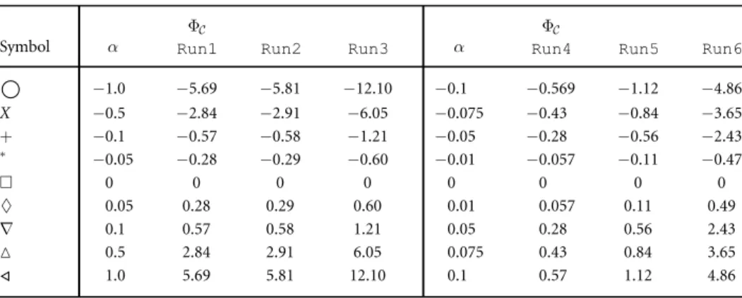
Table A2. Values of the dimensionless numberF from our DNS runs Run1–Run6for nine different values of α. The symbols in the first column serve as guide for the curves in figure5.



F F

Symbol α _{Run1 Run2 Run3} α _{Run4 Run5 Run6}

◯ −1.0 −5.69 −5.81 −12.10 −0.1 −0.569 −1.12 −4.86 X −0.5 −2.84 −2.91 −6.05 −0.075 −0.43 −0.84 −3.65 + −0.1 −0.57 −0.58 −1.21 −0.05 −0.28 −0.56 −2.43 * _{−0.05 −0.28 −0.29 −0.60 −0.01 −0.057 −0.11 −0.47} , 0 0 0 0 0 0 0 0 à 0.05 0.28 0.29 0.60 0.01 0.057 0.11 0.49 ∇ 0.1 0.57 0.58 1.21 0.05 0.28 0.56 2.43 ! 0.5 2.84 2.91 6.05 0.075 0.43 0.84 3.65 ◃ 1.0 5.69 5.81 12.10 0.1 0.57 1.12 4.86