Deconstructing turbulence and optimising GLAO using imaka telemetry

(1)

HAL Id: hal-02340523

https://hal.archives-ouvertes.fr/hal-02340523

Submitted on 15 Dec 2020

HAL is a multi-disciplinary open access archive for the deposit and dissemination of sci-entific research documents, whether they are pub-lished or not. The documents may come from teaching and research institutions in France or abroad, or from public or private research centers.

L’archive ouverte pluridisciplinaire HAL, est destinée au dépôt et à la diffusion de documents scientifiques de niveau recherche, publiés ou non, émanant des établissements d’enseignement et de recherche français ou étrangers, des laboratoires publics ou privés.

Deconstructing turbulence and optimising GLAO using

imaka telemetry

Olivier Lai, Mark Chun, Fatima Abdurrahman, Jessica Lu, Maxwell Service,

Dora Fohring, Douglas Toomey

To cite this version:

Olivier Lai, Mark Chun, Fatima Abdurrahman, Jessica Lu, Maxwell Service, et al.. Deconstructing turbulence and optimising GLAO using imaka telemetry. Adaptive Optics Systems VI, Jun 2018, Austin, TX, United States. pp.229, �10.1117/12.2313356�. �hal-02340523�

(2)

Deconstructing Turbulence and optimizing GLAO using imaka

telemetry

Olivier Lai*

a

_{, Mark Chun}

b

_{, Fatima Abdurrahman}

c

_{, Jessica Lu}

c

_{, Max Service}

b

_{, Dora Fohring}

b

_{, Doug}

Toomey

d

a

_{Université Côte d’Azur, Observatoire de la Côte d’Azur, CNRS, Laboratoire Lagrange, Bd de}

l’Observatoire, CS 34229, 06304 Nice cedex 4, France;

b

_{Institute for Astronomy, University of}

Hawaii, 640 N. Aohoku place, Hilo, HI USA 96720;

c

_{Department of Astronomy, University of}

California, Berkeley, CA USA;

d

_{Mauna Kea Infrared, 21 Pookela Street, Hilo, HI USA 96720}

ABSTRACT

By analyzing global covariance matrices from the imaka GLAO system at the UH 2.2m telescope, it is possible to reconstruct ground layer strength, the integrated turbulence strength as well as the vertical turbulence profile. These are compared to simultaneous profiles obtained by the Maunakea facility MASS/DIMM. A method has been developed to directly compute the phase structure function from the covariances of the slopes, obtained from the telemetry data. The phase structure function allows to test the validity of the Kolmogorov (or van Karman) model and the spatial frequency content of the turbulence: Dome and telescope tube seeing are expected to have an excess of high spatial frequencies, which is detrimental to the PSF by amplifying the halo, and which the AO system cannot correct.

The telescope, the dome and their interaction with the ground layer produce a complex environment for the turbulence. We are therefore developing a small, portable optical turbulence sensor which we will be able to use to scan the dome and telescope tube to quantify the local presence of turbulence. This is the AIR-FLOW (Airborne Interferometric Recombiner - Fluctuations of Light at Optical Wavelengths) project. With imaka and AIR-FLOW we hope to generate a coherent and quantitative account of the turbulence type and strength present in the telescope beam and to accurately match this detailed phase information to the focal plane images. Such a level of detail is required to understand and eventually be able to control the local environment for optimized image quality. We foresee this expertise will be especially valuable for ELTs, where the halo around the PSF will act like an extra source of background.

Keywords: optical turbulence, ground layer adaptive optics, dome seeing, tomography, turbulence profiling

1. INTRODUCTION

Imaka is a ground layer adaptive optics (GLAO) prototype/demonstrator installed at the University of Hawaii 88” telescope on Maunakea [1, 2]. The goal of this project is to analyze and optimize GLAO performance over large fields; indeed, the patrol field of the wavefront sensors is on the order of 0.4˚ (24’ x 18’) and the science field of view is on the order of 12’. Up to 5 Shack Hartman wavefront sensors can be positioned on guide stars; these have 8 x 8 subapertures of 12x12 pixels measuring 0.4” providing a relatively large 5” field, necessary for open loop and GLAO operation. The correction is provided by a 36-electrode bimorph mirror manufactured by CILAS, on loan from Subaru Telescope (it was the DM used in their first-generation facility AO system). Imaka was installed of the UH88” telescope in October 2016 and had its GLAO first light in November 2016. Observing runs took place in January, February and May 2017 (as well as March 2018 but data is not included in present analysis). A detailed description of the instrument can be found in [3] and of its performance in [4]. Here, we focus on the very useful tool of having 5 simultaneous wavefront sensors pointing in different directions to analyze the turbulence through its properties and its profile. This information can be also used to generate tomographic filters, such as a learn-and-apply method adapted from MOAO to GLAO applications. The measurements used were obtained in open loop, although the methods developed herein will be adapted to closed loop operation (by reconstructing pseudo-open loop measurements from the commands to the deformable mirror), where the sensitivity to altitude turbulence may be improved, but the detailed structure of the turbulence near the ground may be harder to extract as the ground conjugate but tilted DM will have a variable height of correction as a function of position in the pupil. The analysis of the turbulence profile follows a method somewhat similar to that developed in [5] and used on the CANARY MOAO instrument on the William Herschell Telescope. Telemetry streams are recorded, containing all relevant

Please verify that (1) all pages are present, (2) all figures are correct, (3) all fonts and special characters are correct, and (4) all text and figures fit within the red margin lines shown on this review document. Complete formatting information is available at http://SPIE.org/manuscripts

Return to the Manage Active Submissions page at http://spie.org/submissions/tasks.aspx and approve or disapprove this submission. Your manuscript will not be published without this approval. Please contact author_help@spie.org with any questions or concerns.

(3)

real time AO variables of interest. These are usually of a length between 1024 and 2048 samples (sometimes multiple telemetry buffers were recorded sequentially, allowing to concatenate the circular buffers); as the sampling frequency is on the order of 180Hz, the buffers sample between 5.5 and 11 seconds of turbulence which may not be sufficient to properly sample the turbulence statistics. Nonetheless, we extract the centroids and compute the slopes covariance matrices: Cslopes = <m.mT>. We call the covariances of each wavefront sensor with itself the auto-covariance and the

covariances of the wavefront sensors with each other the cross-covariances. The former contain the integrated the turbulence and the latter contain information on the ground layer and up to the altitude where the meta-pupil starts to become discontinuous (in practice, the highest levels are only poorly sampled as fewer subapertures are available for their measurement.

2. SLOPE COVARIANCE MATRIX MODEL

The analysis depends on being able to interpret the covariance matrices. To do so, we need a model against which to compare our data. Consider two subapertures of size d and a distance r apart. By virtue of Green’s Theorem, we can write the slope vector s as:

(1)

The contour integral ∮ ϕx dy is the sum (i.e. normalized to the subaperture size, the average

value) of the phase along the left edge of the subaperture ϕ<y>(x) minus the sum of the phase

along the right edge, ϕ<y>(x + d). By virtue of the mean theorem, of the phase along the left

edge can be approximated as the value of the phase halfway along the edge, point A for subaperture 1, point C for subaperture 2; similarly, the average value of the phase on the right side of the subaperture is approximated as the phase halfway along the subaperture, point B for subaperture 1, point D for subaperture 2, so we can write ∮ϕx dy ~ ϕy=A(x) -ϕy=B(x

+ d). To alleviate the notation, we write the x-slope of subaperture 1 as sx1 = ϕ(B) - ϕ(A) and

the x-slope of subaperture 2 as sx2 = ϕ(D) - ϕ(C). We can then write the covariance matrix

of the x-slopes as:

(2) Recall that the phase structure function Dϕ is defined as:

(3)

By writing <ϕ(B) ϕ(D)> as 1/2 Dϕ(BD) - 𝜎𝜙2 , we can replace the covariances of equation 2 by the phase structure functions

and all the variances cancel out:

(4) Similarly, we can compute the y-slope covariances <sy1 sy2> and the x-y covariances, although these contain less

information at small separation. For the phase structure function, we can use either the Kolmogorov or the von Karman models, both of which have relatively straightforward analytical expressions. We can thus generate covariance matrices for layers at any altitude, simply by maintaining the proper geometrical relationship of the subapertures within each beam, through the distance r at the given altitude.

2.1 Direct inversion

It is possible to construct a large altitude-covariance matrix, where each column is the covariance matrix for a layer at a single altitude, unfolded into a vector. Such a matrix A would be of size [Nheight, (2 x Nsubaper x Nwfs)2_{] for which a} generalized inverse of the form A†_{= (A}T_.A)-1_AT_{can be found. In theory, it ought to be possible to multiply a measured} covariance matrix-vector by this generalized inverse and obtain a vector containing the strength of each layer at each altitude of the model. Unfortunately, this method is limited both because the noise in the measurements propagates in the

Figure 1: Two subapertures of side d and a distance r apart.

(4)

reconstruction, but also because the outer scale L0 varies with altitude. Specifically, it can lead to negative values of the

turbulence strength when the off-diagonal response for an altitude layer is too narrow due to a small outer scale. One possible solution is to filter the tip-tilt from the measurements and compute a model covariance matrix with a van Karman spectrum and a small outer-scale, on the order of the telescope diameter, although this still does not prevent the turbulence strength to be negative at times. A disadvantage of filtering the tip-tilt is that information on the outer scale is essentially lost, although in the presence of vibrations, it usually required to filter it to reconstruct the turbulence profile. An advantage of this method is that once the model covariance matrices at altitude are calculated, extracting the profile from the measurements requires a simple matrix multiplication.

2.2 Covariance map fitting

The covariance matrices contain a lot of redundant information and the signal can be increased over the noise by averaging all the matrix elements that represent the same subaperture separation on the pupil. This is simply a reordering and averaging of the matrices but allows to reduce the size of the maps from (2 x Nsubaper x Nwfs)2_{to (2 x Nxsub x Nwfs)}2_{, with} Nsubaper = Nxsub2_.

We first extract integrated properties of the turbulence, by using only the auto-covariance maps. We average the autocovariance maps of all the wavefront sensors under the assumption that the free atmosphere turbulence is independent of the direction of the guide star. We use a simplex algorithm to find the phase structure function that produces the best fit to the measured covariance maps, as given by equation 4. To simplify and constrain the phase structure function, we parametrize using the von Karman model, which has been shown to be representative of many different types of turbulence, indoors or outdoors [6, 7]. We use the formula given by Kellerer [8]:

(5)

with k=6.88. We then average the cross-covariances and the central peak of the covariance map will be due to the ground layer only. We use the same simplex algorithm to obtain the r0 and L0 of the ground turbulence. Once we have found the best fit to the ground layer covariance peak, we subtract it from the integrated covariance peak and estimate the free atmosphere turbulence strength and outer scale.

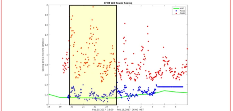
Figure 2: MKAM Mass/DIMM measurement of the turbulence on the night of UT February 16th_{2017. The yellow box shows the time}

span during which we observed. The blue dots show the free atmosphere seeing, below 0.2” on average but with spikes up to 0.4”. The red dots show the ground layer seeing, with two large spikes shortly after 06:00UT (20:00HST) and around 8:00UT (22:00HST).

(5)

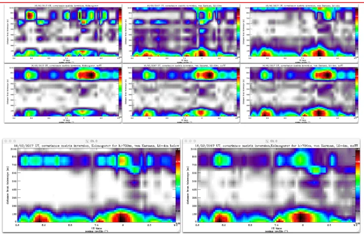
Figure 3: Turbulence profiles for the night of UT20170216, obtained from direct covariance matrix inversion. On the top row from left to right, Kolmogorov, von Karman with L0=20m and L0=4m. The middle row shows the same turbulence models but with tip-tilt filtered. Both have systematic residual seen as horizontal and vertical persistent lines where the method simply fails. The bottom two panels show a hybrid model with a von Karman phase structure function with L0=4m for altitudes below 700m and a Kolmogorov phase structure function above.

Single layers of turbulence at altitude will produce a decentered covariance peak. Using cross-covariance maps from which we have subtracted the ground layer and free atmosphere components, we try to estimate the turbulence profile by fitting our decentered altitude-dependent model covariance maps to these residuals. We use a priori information of the direction in which the secondary peaks are located for each pair of guide star, to increase the sensitivity, but the signal is usually quite tenuous, and it is therefore challenging to extract the outer scale at altitude. Increasing the number of samples in our circular buffers and obtaining very clean covariance maps could alleviate this issue. Note however, that since most of the data from the UH88” telescope is tainted by vibrations the accuracy of the methods only work reliably when tip-tilt is filtered, but L0 is consequently severely underestimated.

It should be possible to remove the vibrations and jitter of the circular buffers from their temporal properties; unfortunately, the temporal power spectrum of tip-tilt shows only a broad peak which is difficult to filter. Also, tip-tilt translates into a constant on the covariance maps, so subtracting a constant should correct this bias, although it is unclear how to estimate the contribution of the turbulence versus the vibrations, and this depends on both r0 and L0. If this could be done to any level of accuracy, then it would also be easy to simply estimate the strength of the turbulence from the modal variance spectrum, which it is not, unless using higher orders, where the effects of the outer scale become negligible.

Running a simplex optimization of r0 and L0 for each altitude is CPU intensive and probably not ideal to implement as a real time tool, although probably provides the best estimates of the turbulence profile (see e.g. Figure 5). Guesalaga et al. [9] have implemented a method where they compute covariance matrices at each altitude for various r0 and L0 and apply a sort of CLEAN peak finding algorithm. We have not implemented such a method but instead, for real time pruposes, we use predetermined outer scales for different altitudes. This method is obviously much faster but will generally overestimate the amount of turbulence near the ground.

(6)

It will be important to obtain good profiles, for example to examine the PSF variability as a function of the thickness of the ground layer. Also, in its current implementation, the learn and apply tomographic filter does require a profile to be optimized, as we use a simulated atmosphere to generate the tomographic filter.

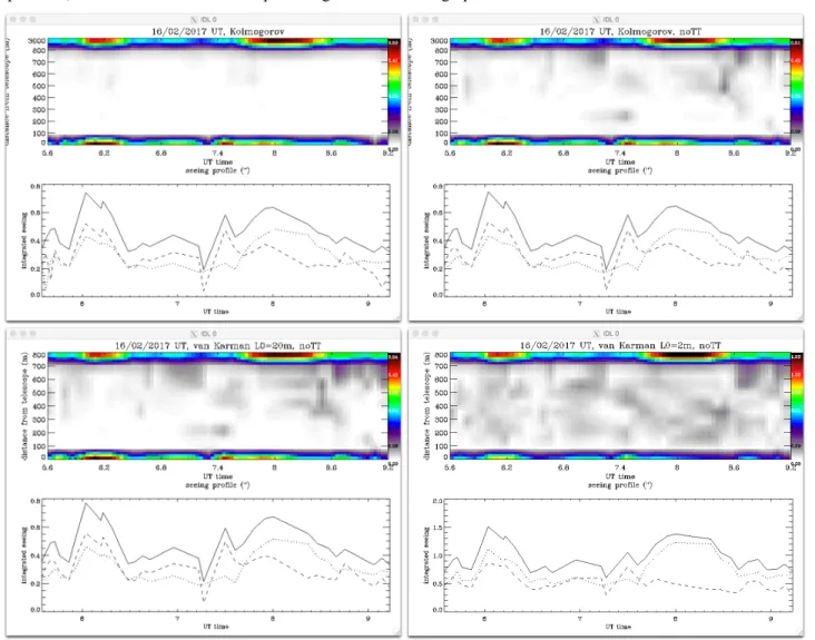
Figure 4: Turbulence profile obtained from Simple fitting of the covariance maps with model covariance maps. We show the results for a Kolmogorov Spectrum on the top row, without (left) and with (right) filtering the tip tilt. The lower row shows the fit of a von Karman phase structure function for L0=20m (left) and 2m (right). In the line plots, the full line is the integrated turbulence, the dashed line is the ground layer and the dotted line is the free atmosphere.

3. TURBULENCE PROFILING

In this section we present some of the turbulence profiles obtained with imaka during the February (for profiles) and May (for spatial properties of the turbulence) observing runs. No statistical study of the profiles has been performed and the data set is not very homogeneous (the three observing runs had very different atmospheric conditions, as well as different guide star constellations, and wavefront sensor orientations). The long-term goal is to have an automated tool that can reconstruct the profiles and populate an archive for statistical analysis and correlation with image plane data.

For comparison purposes, we include the measurements from MASS/DIMM obtained for the night of February 16th_for which we show the profile analysis. That nigh had strong ground layer turbulence and a free atmosphere seeing between 0.1 and 0.4”.

(7)

3.1 Comparison of methods for night of UT20170216

First, we show the profile obtained by direct inversion of the covariance matrix in Figure 3. We have a choice for the model to use and whether to filter the tip tilt or not. Note that filtering tip-tilt means that it is filtered from the covariance matrices in the fitting process, but not from results, so the estimated seeing contains the full turbulence. We find that a hybrid model with a von Karman phase structure function with L0=4m for altitudes below 700m and a Kolmogorov phase structure function above seems to minimize the artefacts, and the filtering of the tip tilt does not alter the results substantially, so this is encouraging. However, the layer at altitude 800m as well as the lack of free atmosphere turbulence (the highest layer represents the free atmosphere and is arbitrarily set to an altitude 3 times higher than the highest reconstructed layer).

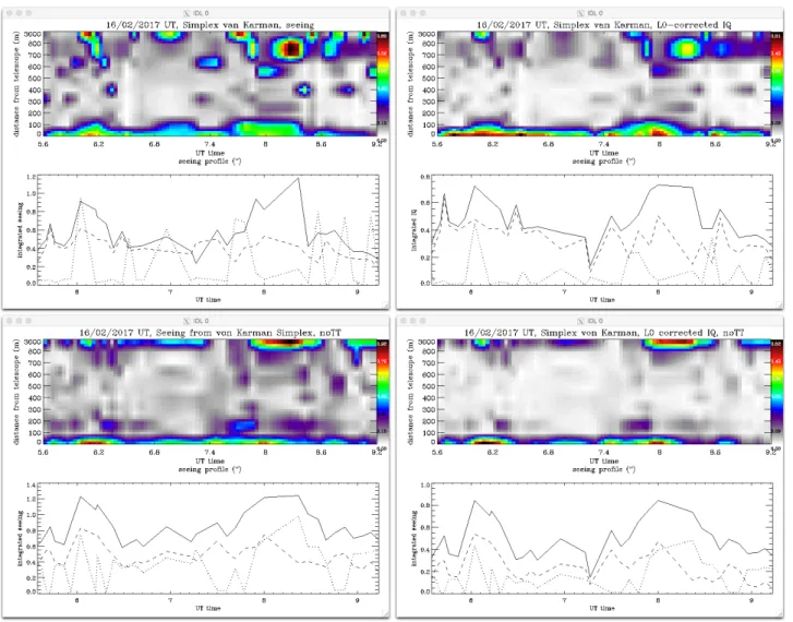
Figure 5: Turbulence profiles obtained by fitting the covariance maps to a von Karman Phase Structure function by Simplex, with r0

and L0 as free parameters at each altitude (top row, with tip-tilt, bottom row, tip-tilt filtered from covariance maps). On the right, we

show the actual IQ, which differs from seeing.

Next in Figure 4, we show the results of our model fitting algorithm (where we set the outer scale to a set value for the model). The main features of Figure 3 are still apparent but the profile is much cleaner, with less noise. Filtering tip-tilt increases the sensitivity to mid-altitude layers, because the off-centered peak become sharper and easier to fit. Reducing the outer scale also seems to increase the sensitivity to mid-altitude layers, for similar reasons. In the same figure we show a plot of seeing (integrated, full line; ground layer, dashed line and free atmosphere, dotted line) because these are each estimated independently of the actual profile. Estimates of these parameters are rather insensitive to which model is being used.

(8)

Finally, we ran the Simplex fitting on the von Karman Model where both r0 and L0 were free parameters shown in Figure 5. Tip-tilt filtering is very time consuming because the covariance maps have to be converted into covariance matrices, for which we can build a tip-tilt filtering matrix. We then have to convert the covariance matrices back into a covariance maps, which prevents this method from being useful in real time. However, for a posteriori analysis, it is the most accurate and most useful as it provides not only the profile of r0 but also that of L0 (Figure 6), and we can start looking for systematic effects that one might expect, such as a smaller outer scale at low altitude.

Seeing is formally defined as the FWHM at 500nm for a Kolmogorov PSF with given r0. However, a finite outer scale modifies (reduces) the FWHM obtained at the focus of the telescope. Since we have access to L0, we can correct for the effect of outer scale on seeing to predict the Image Quality (IQ), to compare directly to the FWHM of focal plane images. (6) This correction factor was established by Martinez et al. [10] and is valid for L0/r0 > 20. However, we show in Figure 6 the actual r0 and L0 obtained as a function of time for both the covariance maps including tip-tilt and those with tip-tilt filtered. A few comments are needed to explain those profiles. The r0 profiles are shown clipped to below 1m; indeed, for r0 much larger than that, the signal of such a weak layer is effectively lost in the noise. Also, when r0 is large, the value of L0 is not very meaningful, since there is no peak in the covariance map to fit. The r0 profiles are qualitatively comparable to the seeing profiles obtained by direct inversion or fixed-model fitting, though we note that the resolution on the ground layer is improved when filtering tip-tilt (as would be expected) but also that the free atmosphere is better estimated when tip-tilt is filtered. The L0 profiles are interesting but rather speculative, as the SNR on the covariance maps obtained with 2048 samples is marginal to fit secondary off-axis peaks. When tip-tilt is included, there are times when the noise is too strong, and the fit is poor for the entire profile (e.g. at UT 6.5, 8.6 and 8.9). However, when filtering tip-tilt the values of L0 are consistently smaller than 20m. It is surprising that the L0 estimates show no correlation to the r0 profiles, as one would expect the noise on L0 to be larger when r0 is large.

The L0 profile is difficult to interpret. However, one thing appears clearly in the bottom left panel of Figure 6: The outer scale of the ground layer is large, quite opposite to what one might have expected. However, tip-tilt adds a constant pedestal to covariance maps, and the apparent large outer scale may be an artefact of the Simplex algorithm trying to fit this pedestal due to vibrations with a von Karman Structure Function, and the one that extends out furthest (effectively acting as a constant in the wings of the covariance maps) is for L0 ↝∞.

Figure 6: r0 (top) and L0 (bottom) profiles with tip tilt (left) and filtered (right). The color scale for r0 is clipped from 0 (black) to 1m

(white) even though some values of r0 are estimated up to 20m. The color scale for L0 goes from 0 to 1000m (left) and from 2 to 10m

(right).

(9)

4. SPATIAL PROPERTIES OF THE TURBULENCE

To further characterize the turbulence, we want to infer its spatial properties, and this is best represented by the phase structure function. A von Karman phase structure function is able to represent most cases of turbulence by varying the outer scale, from ∞ for fully developed, Kolmogorov turbulence to L0~D for random walk, diffusive turbulence. However, since we have a model that allows to get the covariance from the phase structure function, we wanted to see if we could obtain the phase structure function empirically from the covariance maps, in other words, can we solve for Dϕ(r) in terms

of <sx1 sx2> from equation 4? For r=0, we can write:

(6) as Dϕ(d) = Dϕ(-d) and Dϕ(0)=0. Similarly, for r=d,

For r=2d,

Etc… (7)

From which we deduce the following discrete sum:

(8) We can then infer the phase structure function without having to parametrize it. This method however tends to amplify noise at long separations as it effectively performs an integration by linking up the variances of points B, C to get from A to D on Figure 1. Also, whereas we try to reconstruct the entire covariance map using our phase structure function-based model, this method only uses a one-dimensional cut through the covariance map to reconstruct the radial phase structure function, it is not trivial to generalize in two dimensions.

W reconstructed the phase structure function using the covariance matrix for the entire night of 2017/02/16, but instead of separating the ground layer and the free atmosphere from the cross-covariances and the difference between the auto-covariance and the cross-auto-covariance respectively, we tried to use a cleaner method whereby we obtained the integrated seeing from the auto-covariances as previously, but for the free atmosphere we subtracted the pairwise measurements of WFSn to those of WFSn+1: both contain the contribution of the ground layer which should subtract out perfectly, leaving a circular buffer with twice the variance of the free atmosphere. For the ground layer, we concatenated the various wavefront sensors into a single circular buffer and computed the covariance by matching different wavefront sensors:

(9)

Using such covariances, we reconstructed the phase structure function non parametrically from equation 8 and tried fitting it with either a variable exponent power law (of the form (r/r0)𝛼_{, with variable r0 and 𝛼) or with a von Karman spectrum} with a finite outer scale. It was not possible to discriminate between these two models, especially given the coarse sampling of the phase structure function (equal to the number of subapertures, 8 in the case of imaka, and limited baseline imposed by the telescope diameter). In the following we report only on open loop von Karman fit values to alleviate the discussion. In the case of a von Karman fit, it is also possible to fit covariance maps on the profile using our simplex algorithm. We can filter the tip-tilt from the data and from the model covariance maps and we can obtain estimates of r0 and L0 only from higher orders. We expect L0 to be smaller than in the case of the data with vibrations present in the tip-tilt signal. In theory

(10)

it should be possible to compute the covariance map for a power law with tip-tilt subtracted but we did not pursue this, especially as GLAO PSFs seem to be very well fitted by a von Karman phase structure function with a small outer scale.

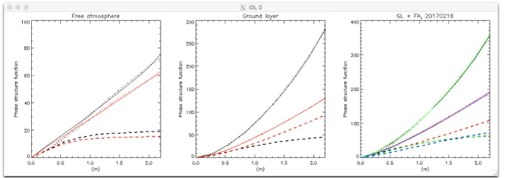
Figure 7: Phase structure functions. In all cases, full line is the phase structure function reconstructed from Equation 8, dotted is the associated von Karman fit while dashed line is the tip-tilt filtered von Karman model fitted to the tip-tilt filtered covariance maps. The red and black curves show x and y for the free atmosphere (left), the ground layer (middle) and the integrated seeing (right); on this last panel green and blue are the integrated seeing (auto-covariances) and black and red are the sum of the left and middle panels. The fact that the red and blue curves, as well as the green and black curves almost overlap means that the integrated seeing matches well the sum of the ground layer and free atmosphere.

In Table 1 and Figure 7 we compare the estimates of r0 and L0 obtained by fitting the tip-tilt-filtered covariance maps with a tip-tilt-filtered von Karman phase structure function to the r0 and L0 computed from fitting the one-dimensional empirical structure function obtained with equation 8.

Table 1: Average values of r0 and L0 for the night of UT February 16th, 0217, obtained from fitting the reconstructed phase structure

function from covariance maps by a von Karman phase structure function. It is worth noting that the vibrations were mostly in x, which may explain the large outer scale for the ground layer along that axis. It is maybe surprising that the outer scale of the free atmosphere is so small.

20170216 Integrated x Integrated y Ground Layer x Ground Layer y Free atmosphere x Free atmosphere y

r0 (m) 0.186 0.186 0.239 0.284 0.256 0.255

L0 (m) 196.0 25.8 2.4 x105 _58.7 _13.1 _10.6

r0_noTT (m) 0.152 0.224 0.223 0.345 0.178 0.171

L0_noTT (m) 5.1 10.1 6.3 57.3 2.7 2.3

The presence of vibrations makes the interpretation of these curves difficult as it prevents a direct comparison of the tip-tilt filtering as well as between x and y. This tool may become useful for systems with a greater number of subapertures, as it will improve the resolution of the reconstructed phase structure function. However, the noise reconstruction of the phase structure function will also increase due to the integration of noisy covariance maps. The phase structure function of tip tilt is a parabola (this is easy to see from first principles since D𝜙2(r) = <| 𝜙(𝜌)-𝜙(𝜌+r)|2_{>, but 𝜙(𝜌+r) = 𝜙(𝜌)} + bx (with b=constant) for pure tip along x-axis, so D𝜙2(r) = <|bx|2_{> = b}2_x2_{and the same for tilt with y).} Unfortunately, it is difficult to separate which part of the tip-tilt comes from vibrations and which is part of the atmosphere. To try to circumvent that, we can also attempt to compute and fit the empirical phase structure function from covariance maps from which we have removed tip-tilt and compare it to fitting the tip-tilt filtered covariance map with a theoretical von Karman covariance map model from which we have not filtered tip tilt. This will certainly introduce a bias in the estimation of the outer scale, but we can at least check for agreement in r0 and between x and y. These results are presented in Figure 8 and Table 2.

(11)

Figure 8: Tip-tilt filtered phase structure functions. As in Figure 8, black is tip (x) and red is tilt (y). Thin full lines are the empirical reconstructed phase structure functions from Equation 8, and the dotted lines are von Karman fits with values reported in Table 2. The dashed lines are von Karman fits on the covariance maps directly, without reconstructing the phase structure functions. Left: free atmosphere, middle: ground layer and right, sum of left and middle panels. On the right panel, green and blue are integrated tip and tilt (respectively) from auto-covariances. The agreement between x and y is much better, indicating the impact of the jitter on the estimation of the phase structure functions.

This work will be greatly improved if we can reduce the telescope vibrations at the source, especially as the jitter is not restricted to a narrow frequency but is spread over a rather band and may even have a low frequency component that is most likely not well sampled given the length of our circular buffers. This jitter also affects the image plane analysis presented in the next section, which, if it were corrected at the source, would allow us to match the telemetry data with the delivered images at the focal plane.

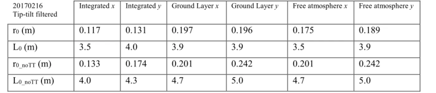
Table 2: r0 and L0 estimated with tip-tilt filtered from circular buffers but not from model, leading to a bias in outer scale.

20170216 Tip-tilt filtered

Integrated x Integrated y Ground Layer x Ground Layer y Free atmosphere x Free atmosphere y

r0 (m) 0.117 0.131 0.197 0.196 0.175 0.189

L0 (m) 3.5 4.0 3.9 3.9 3.5 3.9

r0_noTT (m) 0.133 0.174 0.201 0.242 0.201 0.242

L0_noTT (m) 4.0 4.3 4.7 5.0 4.7 5.0

4.1 Phase structure function from image plane data

To compare the wavefront sensor reconstructed phase structure function, we can try to obtain the phase structure function from focal plane image data. If we call the Optical Transfer Function (OTF) the autocorrelation of the pupil function and the Modulation Transfer Function (MTF) the Fourier transform of the PSF, then the following relations hold:

(9)

Unfortunately, in the case of GLAO (or seeing limited), the MTF does not extend out to the cut-off frequency of the telescope, and the large separations on the phase structure function are dominated by numerical errors by taking the logarithm of an exceedingly small number. However, the small separations on the pupil are adequately estimated, as shown in Figure 9.

(12)

Figure 9: (left) Phase structure function obtained from image plane data on the night of My 18th 2017. Decreasing SNR from cyan to yellow, we can see the saturation of the phase structure function due to numerical errors of the logarithm of small numbers. The small separation regime is well fit by a Kolmogorov phase structure function with r0 of 0.25m.

It is more robust to try to fit the phase structure function in image plane using the Fourier Transform of equation 9. We then have to revert to a parametric phase structure function. In Figure 10, we show the r0 and L0 estimated for the run of May 2017 from image plane data (note that these images are elongated due to jitter and the analysis is only carried out on the narrow axis of the PSF). The range of r0 remains more or less unchanged between open and closed loop, but the outer scale is systematically reduced when the loop is closed (Figure 10, right). This suggests that the GLAO PSF may be well parametrized with a von Karman phase structure function with a small outer scale.

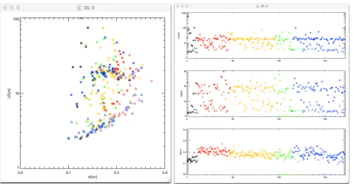
Figure 10: (Left) r0 and L0 obtained from fitting the narrow axis of image plane data for the entire May 2017 run; different colors indicate different nights. Stars are open loop and triangles are closed loop. (Right) r0 and L0 versus time from image data during the

May 2017 run (same color coding). The open (star) and closed (triangle) loop r0 (bottom panel) are almost identical, but the outer scale

(top panel: log scale showing some outliers, middle panel: linear scale) is systematically smaller when GLAO correction is turned on.

Distance (meters) Pha se s tr uc tu re f unc ti on (r ad 2 ) (m et ers )

(13)

Figure 11, left: r0 vs L0 and right: r0 (bottom) and L0 (middle and top) vs. time allowing for PSF broadening in one axis in the phase

structure function by including a parabolic component, the amplitude and angle of which are free parameters of the fit.

Since the fit in the image plane is more robust, we can also try to fit the PSF with a von Karman phase structure function to which we add a parabolic component in one dimension, representative of the broadening of the PSF due to vibrations. We let the amplitude and the angle of the parabola vary as free parameters of the fit and obtain the results shown inFigure 11. A major difference with the results obtained using the narrow axis of the PSF is that the r0 is smaller on average, for both open and closed loop images. The open loop L0 is also smaller, which makes the effect of the GLAO correction as a reduction of the outer scale less visible but compared toFigure 11, it is the estimated closed loop outer scale that remains relatively unchanged, while the open loop outer scale show more variation (indicating that some of the residual tip-tilt from the narrow axis PSF contributes to overestimating L0.

5. TAMING TURBULENCE

The reason why it is important to determine the turbulence profile and the spatial properties of the turbulence is to understand the physical properties of the turbulence, to determine whether the GLAO correction will be useful given the conditions but also to be able to produce optimal tomographic filters and understand which ones will perform better. We currently only consider implementing on two types of tomographic filters (described below), but the goal is to use the imaka prototype as a testbench for different algorithms.

5.1 Tomographic filters

We are developing two approaches to improve GLAO correction by attempting to reject the free atmosphere from the measurements. To do better than simple averaging, we need to include some a priori information, which helps to identify (and reject) turbulence not associated with the ground layer. Turbulence profiles and temporal filtering are such examples. The learn and apply method, developed by Vidal etal, [10] is conceptually very simple: What is the matrix M which will produce the optimal measurements in the center (or any other part) of the field, given a set of measurements on the periphery (or anywhere else): mfield =MLA mWFS. We can multiply both side by mWFST_{and take a time average to find: MLA} = < mfield • mWFS > < mWFS • mWFS >-1_{. The latter term is the inverse of the covariance matrix, which we have access to} (though not always well conditioned), but the former term is harder to obtain. For MOAO applications, a truth sensor can be used at the location of the science target, but in GLAO, it is the average of the field, therefore only the measurements from the ground that we are interested in. We can try to average the measurements of the different WFS to obtain an estimate of the ground layer measurements, but these will still include the partially averaged FA from each direction. We

(14)

propose to estimate mfield by open loop simulations, for which we need to know the thickness (and profile) of the ground layer. Knowing the outer scale is also useful. We draw many realizations of the phase screens maintaining the proper geometrical relationships between guide stars and layer height and can compute learn and apply tomographic filters in this way. We have tried this algorithm on the sky during the May 2017 run, but the results are not conclusive, as too much time had elapsed between obtaining measurements and producing the tomographic matrix.

Another promising method to improve GLAO correction is to use the spatio-temporal covariance maps to identify layers traveling at different speeds and generate a filtering matrix from these covariance maps. Such a filter should allow to isolate layers and their relative speed and only combine measurements from the current and N previous frames that contribute to the signal of these selected layers. We can observe these peaks in spatio-temporal covariance maps and work is ongoing to isolate them automatically and transform them into an optimal filter.

5.2 AIR-FLOW

GLAO performance will be strongly dependent on controlling the wings of the PSF to reduce the NEA as much as possible. The telescope, the dome and their interaction with the ground layer produce a complex environment for the turbulence and it is difficult to interpret data which can intermittently be very different from simple models. The wings of the PSF occur when there is an excess of high spatial frequencies with respect to low ones. This can occur if the outer scale of the turbulence is small, if the turbulence is not fully developed or in the case of diffusive turbulence. All these phenomena occur in the vicinity of or inside the dome, and this is a part of the environment we can control. To better understand the self-generated turbulence, we have developed a portable turbulence sensor, named AIR-FLOW [11]. Such a sensor will also be useful to control the dome vents of telescopes such as CFHT and Gemini, as well as to optimize the airflow in the domes of ELTs.

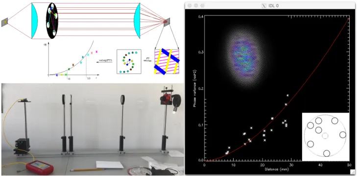
Airborne Interferometric Recombiner – Fluctuations of Light at Optical Wavelength is a turbulence sensor based on a non-redundant mask. Because the baselines are small, the induced turbulence phase perturbations are small. The variance of the phase of each frequency of the Fourier transform of the complex fringe pattern in the focal plane provides an estimate of the variance of the phase (within the linear range) at different separations and allows to measure the phase structure function directly. First tests using a small heat source show promising results (Figure 12). The instrument will be ruggedized and tested simultaneously with INTENSE/LOTUCE [6, 7] at Plateau de Calern before attempting to measure turbulence at the UH88” concurrently with imaka.

Figure 12: First results of the AIRFLOW prototype. A point source is reimaged through a non-redundant mask (lower right inset) and produces the fringe pattern shown on the inset at the top left of the plot. A heat source was placed in the test area and produced the data shown on the right. The red line is a Kolmogorov spectrum.

(15)

6. CONCLUSION

We have presented ongoing work to use wavefront sensor telemetry from imaka to try to reconstruct the optical turbulence seen during our observations, both in its vertical profile as well as its spatial properties. We have presented three different methods to reconstruct the profile using an analytical model of the phase structure function (direct inversion, Simplex with fixed model, Simplex with variable r0 and L0). We have also presented the state of affairs of the estimation of the phase structure function both empirically and with a von Karman parametrization. Work is ongoing to separate the contribution of jitter using Moffat parametrization. We have also tried to estimate the phase structure function from image plane data and found that we cannot access it directly. We can however use a simplex fit to estimate r0 and L0 from the difference between the data and a theoretical PSF computed using a von Karman phase structure function. Because of the presence of vibrations, we can either use the narrow axis of the PSF or try to add a parabolic component to the phase structure function (the amplitude and angle of which are free parameters in the fit). The results of these algorithms are in the process of being integrated to a tomographic filter for GLAO. Finally, we report on the first measurements obtained with our AIRFLOW prototype, the goal of which is to chase down the turbulence inside the telescope dome and tube, and especially attempt to determine its physical properties.

With imaka and AIR-FLOW we hope to generate a coherent and quantitative account of the turbulence type and strength present in the telescope beam and to accurately match this detailed phase information to the focal plane images. Such a level of detail is required to understand and eventually be able to control the local environment for optimized image quality. We foresee this expertise will be especially valuable for ELTs, where the halo around the PSF will act like an extra source of background.

REFERENCES

[1] Lai, O., Chun, M., Cuillandre, J.-C., Carlberg, R., Richer, H., et al, "IMAKA: imaging from Mauna KeA with an atmosphere corrected 1 square degree optical imager," Proc. SPIE 7015, 70154H (2008).

[2] Chun, M.R., Lai, O., Toomey, D., Lu, J., et al, “imaka: a ground layer adaptive optics system on Mauna Kea,” Proc. SPIE 9909, 990902 (2016).

[3] Chun, M.R., et al, in preparation (2018).

[4] Abdurrahman, F., Lu, J.R., Chun, M., Service, M., Lai, O., et al, “Improved Image Quality over 10’ fields with the `Imaka ground layer adaptive optics experiment,” Astrophys. J., submitted (2018).

[5] Martin, O.A., Correia, C.M., Gendron, E., Rousset, G., Vidal F., et al, “William Herschel Telescope site characterization using the MOAO pathfinder CANARY on-sky data”, Proc SPIE 9909, 99093P (2016)

[6] Ziad, A., Dali Ali, W., Borgnino, J., Sarazin, M., Buzzoni, B., “Lotuce: a new monitor for turbulence characterization inside telescope’s dome,” Proc. AO4ELT3, 79 (2013)

[7] Chabé, J., Blary, F., Ziad, A., Borgnino, J., Fantei-Caujolle, Y., Liotard, A., Falzon, F., “The INdoor TurbulENce SEnsor (INTENSE) instrument”, Proc SPIE 9145, 91453A (2014)

[8] Kellerer, A., “A Cookbook of Structure Functions”, arXiv:1504.00320 [physics.data-an] (2015)

[9] Guesalaga, A., Neichel, B., Correia, C.M., Butterley, T., Osborn, J., Masciadri, E., Fusco, T., Sauvage, J.-F., “Online estimation of the wavefront outer scale profile from adaptive optics telemetry”, MNRAS, 465, 1984-1994 (2017) [10] Martinez, P., Kolb, J., Tokovinin, A., Sarazin, M., “Atmospheric blur with finite outer scale or partial adaptive optics

correction”, Astron. Astrophys., 516, A90 (2010)

[11] Vidal, F., Gendron, E., Brangier, M., Sevin, A., Rousset, G., Hubert, Z., “Tomography reconstruction using the learn and apply algorithm”, Proc AO4ELT1, 07001, (2010)

[12] Lai, O., Chun, M., Withington, K., “AIR-FLOW: Airborne Interferometric Recombiner: Fluctuations of Light at Optical Wavelengths”, Proc. SPIE 9909, 99093H, (2016)