Quasi-Symplectic Langevin Variational Autoencoder

(1)

HAL Id: hal-03024748

https://hal.inria.fr/hal-03024748v3

Preprint submitted on 19 Apr 2021 (v3), last revised 3 Jun 2021 (v4)

HAL is a multi-disciplinary open access

archive for the deposit and dissemination of

sci-entific research documents, whether they are

pub-lished or not. The documents may come from

teaching and research institutions in France or

abroad, or from public or private research centers.

L’archive ouverte pluridisciplinaire HAL, est

destinée au dépôt et à la diffusion de documents

scientifiques de niveau recherche, publiés ou non,

émanant des établissements d’enseignement et de

recherche français ou étrangers, des laboratoires

publics ou privés.

To cite this version:

Zihao Wang, Hervé Delingette. Quasi-Symplectic Langevin Variational Autoencoder. 2021.

�hal-03024748v3�

(2)

Q

UASI

-

SYMPLECTIC

L

ANGEVIN

V

ARIATIONAL

A

U

-TOENCODER

Zihao WANG∗

Inria Sophia Antipolis, University Cˆote d’Azur 2004 Route des Lucioles, 06902 Valbonne zihao.wang@inria.fr

Herv´e Delingette

Inria Sophia Antipolis, University Cˆote d’Azur 2004 Route des Lucioles, 06902 Valbonne herve.delingette@inria.fr

A

BSTRACT

Variational autoencoder (VAE) is a very popular and well-investigated generative model vastly used in neural learning research. To leverage VAE in practical tasks dealing with a massive dataset of large dimensions it is required to deal with the difficulty of building low variance evidence lower bounds (ELBO). Markov Chain Monte Carlo (MCMC) is one of the effective approaches to tighten the ELBO for approximating the posterior distribution. Hamiltonian Variational Autoencoder (HVAE) is an effective MCMC inspired approach for constructing a the low-variance ELBO which is also amenable to the reparameterization trick. In this work, we propose a Quasi-symplectic Langevin Variational autoencoder (Langevin-VAE) by incorporating the gradients information in the inference process through Langevin dynamic. We shows the effectiveness of the proposed approach by toy and real world examples.

1 I

NTRODUCTION

Variational Autoencoders (VAE) are a popular generative neural model applied in a vast number of practical cases to perform unsupervised analysis and to generate specific dataset. It has the advantages of offering a quantitative assessment of generated model quality and being less cumbersome to train compared to Generative Adversarial Networks (GANs). The key factor influencing the performance of VAE models is the quality of the ,arginal likelihood approximation in the corresponding evidence lower bound (ELBO). A common method to make the amortized inference efficient is to constraint the posterior distribution of the latent variables to follow a given closed-form distribution, often multivariate Gaussian (Wolf et al., 2016). However, this severely limits the flexibility of the encoder. In (Salimans et al., 2015), the Hamiltonian variational inference is proposed to remove the requirement of an explicit formulation of the posterior distribution by forward sampling a Markov chain based on Hamiltonian dynamics. It can be seen as a type of normalizing flows (NFs) (Rezende & Mohamed, 2015) where repeated transformations of probability densities are replaced by time integration of space and momentum variables. To guarantee the convergence of HVI to the true posterior distribution, Wolf et al. proposed to add an acceptance step in Hamiltonian variational inference algorithm. In (Caterini et al., 2018), authors first combined VAE and HVI in Hamiltonian Variational Autoencoders (HVAE) which include a a dynamic phase space where momentum component ρ and position component z are integrated which introduces the target information into the flow. Briefly, HVAE employs a K steps Hamiltonian HK transformation process to build an unbiased estimation of

posterior q(z) by extending ˜p(x, z) as ˜p(x, HK(z0, ρ0)) leading to: ˜p(x) := ˆ

p(x,HK(z0,ρ0))

q(HK(z0,ρ0)) , where:

ˆ

p(x, zK, ρK) = ˆp(x, HK(z0, ρ0)) = ˆp(x, zK)N (ρK|0, I). HVAE in particular, allows the use of

the reparameterization trick during inference thus leading to efficient ELBO gradients computation. In this work, as an exploration of the application of dynamic systems in the field of machine learning, we propose a novel inference framework named quasi-symplectic Langevin variational auto-encoder (Langevin-VAE) that leads to both reversible Markov kernels and phase quasi-volume invariance similarly to Hamiltonian flow (Caterini et al., 2018) while reducing the computation and memory requirements. The proposed method is a low-variance unbiased lower bound estimator for

∗

(3)

infinitesimal discretization steps but needs just one target Jacobian calculation and avoids computing the Hessian of Jacobian. The leapfrog integrator of Hamiltonian flows is replaced in our approach by the quasi-symplectic Langevin integration.We show that the Langevin-VAE is a generalized stochastic inference framework since the proposed Langevin-VAE becomes symplectic when the viscosity coefficient ν = 0 is set to zero. The method is verified through quantitative and qualitative comparison with HVAE inference framework on a benchmark dataset.

2 P

RELIMINARY

2.1 VARIATIONALINFERENCE ANDNORMALIZINGFLOW

One core problem in the Variational Inference (VI) task is to find a suitable replacement distribu-tions qθ(z) of the posterior distribution p(z|x) for optimizing the ELBO: argmaxθEq[log p(x, z) −

log qθ(z)]. To tackle this problem, Ranganath et al. proposed black box variational inference

by estimating the noisy unbiased gradient of ELBO to perform direct stochastic optimization of ELBO. Kingma & Welling proposed to use some multivariate Gaussian posterior distributions of latent variable z generated by a universal function ω, which makes reparameterization trick is pos-sible: argmax_θ,φEqθ(z|x)[log pθ(x, z) − log qφ(z|x)]. To better approximate potentially complex

posterior distributions of latent variables, the use of simple parametric distributions like multivariate Gaussian is a limitation. Yet only a few of distributions are compatible with the reparameterization trick. Normalizing Flows (NFs) Rezende & Mohamed was proposed as a way to deal with more gen-eral parametric posterior distributions that can still be efficiently optimized with amortized inference (Papamakarios et al., 2019). NFs are a class of methods that use a series of invertible transformation TK... ◦ ...T0to map a simple distribution z0 into a complex one zk: zk = TK... ◦ ...T0(z0), By

applying a cascade of transformations, the corresponding logarithm prior probability p(zk) of the

transformed distribution becomes:

ln(p(zk)) = log(p(z0)) − Σk0log det ∂Tk ∂zk−1 (1) where the non-zero Jacobian |det ∂Tk

∂zk−1| of each transformation ensures the global volume invariance

of the probability density. The positivity of each Jacobian terms is guaranteed by the invertibility of each transformation T and consequently by the reversibility of normalizing flows.

The Hamiltonian dynamics in HVAE can also be seen as a type of NFs, for which Eq: (1) also holds. The Hamiltonian flow samples the posterior distribution p(z|x) as the trajectory of a particle evolving as an Hamiltonian dynamical system under the potential energy given by U (x, z) = − log p(x, z) given an initial momentum ρ0. The Hamiltonian dynamics is such that the distribution of phase space

z, ρ remains constant along each trajectory according to Liouville’s theorem (symplectic) (Fass`o & Sansonetto, 2007). When using the leapfrog integrator with step size l for discretizing the Hamil-tonian dynamics, the Jacobian remains closed to 1 with liml→0|det∂T_∂zk

k|

−1

l = 1. This property

simplifies the Jacobian calculations at each discretization step (Caterini et al., 2018). In HVAE, the posterior approximation is constructed by applying K steps of the Hamiltonian flow (Caterini et al., 2018): qK_(H

k(θ0, ρ0)) = q0(Hk(θ0, ρ0))Q K

k=1|det∇Φ k_(H

k(θ0, ρ0))|−1, where Φkrepresents the

leapfrog discretization transform of Hamiltonian dynamics. When combined with the reparameteriza-tion trick, it allows to compute an unbiased estimator of the lower bound gradients ∇θL. Yet, since the leapfrog integrator involves two split sub-steps to update the momentum (Girolami & Calderhead, 2011), the computation of the lower bound gradient requires 2 × K computations of the Jacobian ∇U .

2.2 LANGEVINMONTE-CARLO ANDNORMALIZINGFLOW

In molecular physics, Langevin dynamics is a stochastic process that models the diffusion of free particles within a potential field U (x) through a Stochastic Differential Equation (SDE): m∂v/∂t := −∇U − γv + η, involving the particle velocity v, its acceleration ∂v/∂t, damping factor γ and environmental noise η. Overdamped Langevin dynamics is obtained when the damping term is much greater than the inertial one leading to a first order SDE : γv = −∇U + η.

As Langevin dynamics describes a stochastic evolution of particles be acted in the particle interaction potential U (x) that can be treated as a log probability density, it has recently attracted a lot of attention

(4)

in the machine learning community (Stuart et al., 2004; Girolami & Calderhead, 2011; Welling & Teh, 2011; Mou et al., 2020) for the stochastic sampling of posterior distributions pΦ(z|x) in Bayesian

inference. Langevin Monte-Carlo methods (Girolami & Calderhead, 2011) rely on the construction of Markov chains with stochastic paths parameterized by Φ based on the discretization of the following Langevin–SmoluchowskiSDE (Girolami & Calderhead, 2011) related to the overdamped Langevin dynamics :

δΦ(t) = 1

2∇Φlog(p(x, Φ))δt + δσ(t) (2)

where σ(t) is a Wiener process and t represents the time. The stochastic flow in Eq (2) can be further exploited to construct Langevin dynamics based normalizing flow and its derived methods for posterior inference (Wolf et al., 2016; Kobyzev et al., 2020). The concept of Langevin normalizing flow was first briefly sketched by Rezende & Mohamed (2015) in their seminal work (in section 3.2). To the best of our knowledge, little work has explored practical implementations of Langevin normalizing flows. In (Gu et al., 2019), the authors proposed a Langevin normalizing flow where invertible mappings are based on overdamped Langevin dynamics discretized with the Euler–Maruyama scheme. The explicit computation of the Jacobians of those mappings involves the Hessian matrix of log(pΦ(x))

as follows : log det ∂Tk ∂zk−1 −1 ∼ ∇z∇zlog(p(x, z)) + O(z) (3)

Yet, the Hessian matrix appearing in Eq (3) is expensive to compute both in space and time and adds a significant overhead to the already massive computation of gradients. This makes the method of (Gu et al., 2019) fairly unsuitable for the inference of complex models.

In a more generic view, in the Langevin flow, the forward transform is modelled by the Fokker-Plank equation and the backward transform is given by Kolmogorov’s backward equation which is discussed in the work of Kobyzev et al. and is not detailed here.

2.3 QUASI-SYMPLECTICLANGEVIN ANDCORRESPONDINGFLOW 2.3.1 QUASI-SYMPLECTICLANGEVINTRANSFORM

To avoid the computation of Hessian matrices in Langevin normalizing flows, we propose to revert to the undamped or generalized Langevin dynamic process as proposed in (Sandev T., 2019). It involves second order dynamics with inertial and damping terms:

δΦ(t) = Kδt

δK(t) = −∂ln(p(x, Φ))

∂Φ δt − νK(t) + δσ(t)

(4)

where Φ(t) and K(t) are the stochastic position and velocity fields, and ν controls the amount of damping. We can see that the Langevin–Smoluchowski type SDE: (2) is nothing but the special case of high friction motion (Sandev T., 2019) when Eq: (4) has an over-damped frictional force. Indeed, since δK(t) = ∂φ(t)_∂t22, in the case of an over-damped system, the frictional force νK

overwhelms the inertial force : δ2θ/δt2_{νK(t). According to the generalized Langevin diffusion}

equation, we have : ∂Φ(t)2 ∂t2 νK(t) = ∂ log(p(x,Φ)) ∂Φ dt νK(t) − 1 + δσ(t) νK(t) Therefore, we get : νK(t) = νδΦ ≈ ∂ log(p(x, Φ)) ∂Φ dt + δσ(t)

To get simple Jacobian expressions when constructing Langevin flow, we need to have a symplectic Langevin transformation kernel. To this end, we introduce a quasi-symplectic Langevin method for building the flow (Milstein et al., 2002). The quasi-symplectic Langevin differs from the Eu-ler–Maruyama integrator method which diverges for the discretization of generalized Langevin SDE. Instead, the quasi-symplectic Langevin method makes the computation of the Jacobian tractable

(5)

during the diffusion process and keeps approximate symplectic properties for the damping and external potential terms.

More precisely, the quasi-symplectic Langevin integrator is based on the two state variables (Ki, Φi)

that are evolving according to the mapping Ψσ(Ki, Φi) = (Ki+1, Φi+1) where σ is the kernel

stochastic factor. It is known as the second order strong quasi-symplectic method (5) and is composed of the following steps for a time step τ :

KII(t, p) = pe−νt K1,i= KII( τ 2, Ki); Φ1,i= Φi− τ ∂ log(p(x, Φ)) 2∂Φ K2,i= K1,i+ √ τ σξi; ξi∼ N (0, I) Ki+1= KII( τ

2, K2,i); Φi+1= Φ1,i+ τ 2K2,i

(5)

where initial conditions are K0= κ0; Φ0= φ0. To guarantee the reversibility of the defined kernel,

the mapping has to be deterministic and therefore we use σ = 0 in the remainder. The above quasi-symplectic integrator satisfies the following two properties:

Property 1. Quasi-symplectic method degenerates to a symplectic method when ν = 0. Property 2. Quasi-symplectic Langevin transform Ψ0(Ki, Φi) (5) has constant Jacobian :

|Ψ0(Ki, Φi)| = ∂Φi+1 ∂Φi ∂Ki+1 ∂Ki −∂Φi+1 ∂Ki ∂Ki+1 ∂Φi = exp(−ντ ) (6)

The first property shows that the VAE constructed based on the Quasi-Symplectic Langevin (QSL) dynamics is conceptually equivalent to a HVAE in the absence of damping ν = 0. The second property implies that the QSL integrator leads to transformation kernels that are reversible and with trivial Jacobians. The proofs of those two properties can be found in Milstein (2003).

The advantage of the QSL flow compared to the regular overdamped Langevin flow is that it avoids computing the Hessian of the log probability to compute the Jacobian which is a major advantage given the complexity of the Hessian computation.

We give the below formal definition of the quasi-symplectic Langevin normalizing flow.

Definition. A K steps discrete quasi-symplectic Langevin normalizing flow LK_{is defined by a series}

of diffeomorphism, bijective and invertible mappingΨ0: σA−→ σBbetween two measurable spaces

(A, σA, µα) and (B, σB, µβ):

LK_µ

α(SA) :Ψi◦ µα(SA) = µα(Ψ−1i−1(SB)),

∀SA∈ σA, SB∈ σB, i = {1, ..., K}.

(7) whereσ(·)andµ(·)are theσ-algebra and probability measure for set (·) respectively, Ψiis theith

quasi-symplectic Langevin transform given by Eqs:(5).

2.3.2 EXAMPLE FOR SINGLE STEP QUASI-SYMPLECTICLANGEVIN FLOW

We illustrate below definition 2.3.1 of a quasi-symplectic Langevin normalizing flow in case of a single transform applied on a single random variable. We consider a probability measure p(x) of random variable set x ∈ X. Then a single step Langevin flow transforms the original random variable x to a new random variable y = Ψ0(x), y ∈ Y . According to definition 2.3.1, the new probability

measure q(y) of random variable y is given by:

q(y) = L0p(x) : Ψ0◦ p(x) = p(Ψ−10 (y)) (8)

By Eq.(1), we conclude that:

q(y) = p(x) · |det∂Ψ0 ∂x |

−1 ₍₉₎

The defined symplectic Langevin flow is a generalization of the Langevin flow with a quasi-symplectic structure for the parameters phase space. The quasi-quasi-symplectic Langevin normalizing flow has a deterministic kernel Ψ0when the kernel stochastic factor σ = 0, and degenerates to a

symplectic transition when ν = 0. With a deterministic kernel, the flow will be able to have the probability density evaluated.

(6)

3 Q

UASI

-

SYMPLECTIC

L

ANGEVIN

VAE

3.1 LOWERBOUNDESTIMATIONWITHLVAE

In the quasi-symplectic Langevin VAE, we use an augmented latent space consisting of position φK

and velocity κK variables of dimension ζ : z = (φK, κK). The objective of the autoencoder is to

optimize its parameters as to maximize the evidence lower bound ˜L:

log p(x) = log Z Ω p(x, z)dz = log Z Ω ˜ p(x)q(˜z|x)d˜z ≥ Z Ω log ˜p(x)q(˜z|x)d˜z ≡ ˜L (10)

where Ω is the measure space of the latent variables and as ˜p(x) is an unbiased estimator for p(x). The lower bound is equal to the evidence when the posterior approximation is equal to the true posterior. Thus maximizing the lower bound is equivalent to minimize the gap between the true posterior p(z|x) and its approximation q(z|x) (Blei et al., 2017).

Algorithm 1: Quasi-symplectic Variational Inference

Inputs: Data X, Inference steps K, damping ν, time step τ , prior q0 ωE(φ0)

Output: Encoding and decoding parameters ω = (ωE, ωD)

Initialize all parameters, variables; Define: KII(t, p) = pe−νt;

while NOT ω converged do Get minibatch: XN N ←− X; while NOT j = N do xj j ←− XN ; // Get xj in minibatch.

φ0∼ qω0E(φ0|xj) ; // Sampling latent variable from variational

prior

κ0∼ N (0, Iζ) ; // Sampling velocity from unit Gaussian.

for i = 1; i < K; i + + do

// Quasi-symplectic Langevin Normalizing Flow κ1,i← KII(τ₂, κi); φ1,i← φi− τ

∂ log(p(x,φ))

2∂φi ;

κi+1← KII(τ₂, κ1,i); φi+1← φ1,i+τ₂κ1,i;

end

p∗ω← ˆpωD(x, φK) · N (κK|0, Iζ);

q∗_ω← q0

ωE(φ0) · N (κ0|0, Iζ)exp(ντ );

˜

L∗j ← ln(p∗ω) − ln(q∗ω); ; // Quasi-symplectic Langevin ELBO

j ← j + 1 end

˜

L∗←PNi=1L˜ ∗

i/N ; // Minibatch average ELBO

arg max_ω∈Rn_L˜∗; // Optimize average ELBO over parameters subset

end

The posterior approximation q(z) is computed through a series of Langevin transformations which is the Langevin flow: qωE(z|x) = q

K_(LK_(φ 0, κ0)) = q0ωE(φ0, κ0|x) QK k=1|det∇Ψ0(φk, κk))|−1= q0 ωE(φ0, κ0|x) exp(Kντ ), where q 0

ωE(φ0, κ0|x) is an initial approximation parameterized by ωE

which can also be seen as the prior on random variables φ0, κ0.

Similarly to the HVAE (Caterini et al., 2018), an unbiased estimator of p(x) is given by :

˜ p(x) = p(x, Lˆ K_(θ 0, k0)) q0 ωE(θ0, κ0) (11)

(7)

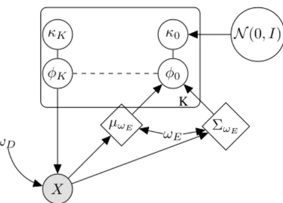
X φK φ0 ΣωE µωE ωE κ0 N (0, I) κK ωD K

Figure 1: Graphical model of the Quasi-symplectic Langevin Variational Autoencoder. The multivari-ate Gaussian parameters µωE, ΣωEdefining the variational prior of latent variable φ0are determined

from the data X and the parameter ωEof the encoding network. The initial velocity latent variable

κ0has a unit Gaussian prior and is paired by initial latent variable φ0. After iterating K times the

quasi-symplectic Langevin transform, the latent pair {φK, κK} is obtained from the initial variables

{φ0, κ0}. The decoder network with parameters ωDis then used to predict the data from latent

variables φKthrough the conditional likelihood p(x|φK). Variables in diamonds are deterministically

computed. Network parameters ωE, ωDare optimized to maximize the ELBO.

We then give the lower bound for the quasi-symplectic Langevin VAE as : ˜ L := Z Ω qωE(˜z|x) · (log ˆp(x, L K_(φ 0, k0))− log(q_ω0 E(φ0, k0)) + Kντ d˜z (12)

3.2 QUASI-SYMPLECTICLANGEVINVAE

The quasi-symplectic Langevin lower bound ˜L lays the ground for the stochastic inference of a variational auto-encoder. Given a set of dataset X : {xi _{∈ X; i ∈ N}

+}, we aim to learn a

generative model of that dataset from a latent space with the quasi-symplectic Langevin inference. The generative model p(x, z) consists of a prior on initial variables z0= (φ0, κ0), qω0E(φ0, κ0|x) =

q0ωE(φ0|x) · N (κ0|0, Iζ) and conditional likelihood pωD(x|z) parameterized by ωD. The Gaussian

unit prior N (κ0|0, Iζ) is the canonical velocity distribution from which the initial velocity of the

Langevin diffusion will be performed. The distribution q0

ωE(φ0|x) is the variational prior that

depends on the data xi_{. Thus the generative model p}

ωE,ωD(x, z) is parameterized by both encoders

and decoders and the quasi-symplectic Langevin lower bound writes as: arg max ωE,ωD ˜ L∗=Eφ0∼q0_ωE(),κ0∼Nζ()(ln ˆpωE,ωD(x, L K (φ0, κ0))− ln(q0_ω_E(φ0, κ0)) + Kντ ) (13)

The maximization of the lower bound (13), is can be performed efficiently with the reparameterization trick depending on the choice of the variational prior qω0E(φ0). To have a fair comparison with prior

work(Caterini et al., 2018), we also perform Rao-Blackwellization for reducing the variance of the ELBO in the quasi-symplectic Langevin VAE:

arg max ωE,ωD ˜ L∗=Eφ0∼q0_ωE(),κ0∼Nζ()(ln ˆpωE,ωD(x, L K_(φ 0, κ0)) − ln(ˆqωE(φ0, κ0)) + Kντ − 1 2κ T KκK) + ζ 2; ∀φ0, κ0∈ R ζ (14)

(8)

4 E

XPERIMENT AND

R

ESULT

We examine the performance of quasi-symplectic Langevin VAE on the MNIST dataset (LeCun et al., 2010) based on various metrics. Caterini et al. (2018) have reported that the Hamiltonian based stochastic variational inference outperforms that of Planar Normalizing Flow, mean-field based Variational Bayes in terms of model parameters inference error and quantitatively shown that the HVAE outperforms the naive VAE method in terms of Negative Log-likelihood (NLL) score and ELBO. Here, we compare the proposed LVAE with the HVAE on MNIST dataset. The experiments were implemented with TensorFlow 2.0 and TensorFlow Probability framework to evaluate the proposed approach in both qualitative and quantitative metrics.

Figure 2: Quantitative result of Langevin VAE in comparison with HVAE. Left sub-figures are generated samples of HVAE. Right are samples of Langevin-VAE. In both methods, the number of steps in the flow computation is K = 5.

Table 1: Quantitative evaluation of the Langevin-VAE in comparison with the HVAE. It includes the comparison of the negative log likelihoods (NLL), the evidence lower bound (ELBO), the Fr´echet Inception (FID) and Inception Score (IS)

Langevin-VAE HVAE Flow steps 1 5 10 1 5 10 NLL 89.41 88.15 89.63 89.60 88.21 89.69 ELBO -91.74 -90.14 -92.03 -91.91 ± 0.01 -90.41 -92.39 ± 0.01 FID 52.70 52.95 53.13 53.12 53.26 53.21 IS 6.42 6.49 6.30 6.57 6.42 6.11

4.1 QUASI-SYMPLECTICLANGEVINVAEON BINARY IMAGE BENCHMARK Given a training dataset X : {xi_{∈ X; i ∈ N}

+} consisting of binary images of size d, xi∈ {0, 1}d,

we define the conditional likelihood p(x|z) as a product of d Bernoulli distributions. More precisely, we consider a decoder neural network DecωD(φ) ∈ [0, 1]

d _{that outputs d Bernoulli parameters}

from the latent variable φ ∈ Rζ _{where z = (φ, κ). Then the conditional likelihood writes as :}

p(xi_|zi_{) =}Qd j=1DecωD(φ)[j] xi_[j] (1 − DecωD(φ)[j]) 1−xi_[j] .

Following the classical VAE approach (Kingma & Welling, 2014), the encoder network parameterized by ωEoutputs multivariate Gaussian parameters : µωE(x) ∈ R

ζ _{and Σ}

ωE(x) ∈ R

ζ_{, such that the}

variational prior is a multivariate Gaussian qω0E(φ0|x) = N (φ0|µωE(x), ΣωE(x)) with diagonal

covariance matrix. This choice obviously makes the reparameterization trick feasible to estimate the lower bound. The related graphical model of the quasi-symplectic Langevin VAE is displayed in Fig. 1.

The decoder and encoder neural network architectures are similar to the HVAE (Caterini et al., 2018) and MCMCVAE (Salimans et al., 2015), both having three layers of 2D convolutional neural networks for encoder and decoder, respectively. The encoder network accepts a batch of data of size (Nb× 28 × 28) with Nb= 1000. The dimension of latent variables is set as ζ = 64 and the damping

factor is ν = 0. The discretization step is τ = 1e − 2. The training stage stops when the computed ELBO does not improve on a validation dataset after 100 steps or when the inference loop achieves 2000 steps.

Both tested models LVAE and HVAE share the same training parameters. The stochastic ascent of the ELBO is based on the Adamax optimizer with a learning rate lr = 5e − 5. All estimation of computation times were performed on one NVIDIA GeForce GTX 1080 Ti GPU. For memory usage evaluation the experiment was performed on a NVIDIA Quadro M2200 GPU.

(9)

4.2 RESULT

Both qualitative and quantitative results are studied. The generated samples of Langevin-VAE and HVAE are shown in Fig: (2). We qualitatively see that the quality and diversity of the sampled images are guaranteed for both autoencoder models. Quantitatively, Table 1 shows the performance in terms of the NLL, ELBO, FID, IS scores for Langevin-VAE and HVAE where Langevin and Hamiltonian flows are experimentally compared.

5 C

ONCLUSION

In this paper, we propose a new flow-based Bayesian inference framework by introducing the quasi-symplectic Langevin flow for the stochastic estimation of a tight ELBO.

By introducing the quasi-symplectic Langevin dynamics, we also overcome the limitation of the Langevin normalizing flow (Gu et al., 2019) which requires to provide the Hessian matrix ∇∇log(p(x, φ)) to compute the Jacobian. Potential improvements of the quasi-symplectic Langevin inference can arise by investigating the manifold structure of the posterior densities of the latent variables (Girolami & Calderhead, 2011; Barp et al., 2017; Livingstone & Girolami, 2014) to improve the inference efficiency.

ACKNOWLEDGMENTS

This work was partially funded by the French government through the UCA JEDI ”Investments in the Future” project managed by the National Research Agency (ANR) with the reference number ANR-15-IDEX-01, and was supported by the grant AAP Sant´e 06 2017-260 DGA-DSH.

R

EFERENCES

Alessandro Barp, Francois-Xavier Briol, Anthony Kennedy, and Mark Girolami. Geometry and dynamics for markov chain monte carlo. Annual Review of Statistics and Its Application, 5, 05 2017. doi: 10.1146/annurev-statistics-031017-100141.

David M. Blei, Alp Kucukelbir, and Jon D. McAuliffe. Variational inference: A review for statisticians. Journal of the American Statistical Association, 112(518):859–877, 2017. doi: 10.1080/01621459. 2017.1285773. URL https://doi.org/10.1080/01621459.2017.1285773. Anthony L. Caterini, Arnaud Doucet, and Dino Sejdinovic. Hamiltonian variational auto-encoder. In

NeurIPS, 2018.

Francesco Fass`o and Nicola Sansonetto. Integrable almost-symplectic hamiltonian systems. Journal of Mathematical Physics, 48(9):092902, 2007. doi: 10.1063/1.2783937. URL https://doi. org/10.1063/1.2783937.

Mark Girolami and Ben Calderhead. Riemann manifold langevin and hamiltonian monte carlo methods. Journal of the Royal Statistical Society: Series B (Statistical Methodology), 73(2):123– 214, 2011. doi: 10.1111/j.1467-9868.2010.00765.x. URL https://rss.onlinelibrary. wiley.com/doi/abs/10.1111/j.1467-9868.2010.00765.x.

Minghao Gu, Shiliang Sun, and Yan Liu. Dynamical sampling with langevin normalization flows. Entropy, 21:1096, 11 2019. doi: 10.3390/e21111096.

Diederik P. Kingma and Max Welling. Auto-encoding variational bayes. In 2nd International Conference on Learning Representations, ICLR 2014, Banff, AB, Canada, April 14-16, 2014, Conference Track Proceedings, 2014. URL http://arxiv.org/abs/1312.6114. I. Kobyzev, S. Prince, and M. Brubaker. Normalizing flows: An introduction and review of current

methods. IEEE Transactions on Pattern Analysis and Machine Intelligence, pp. 1–1, 2020. Yann LeCun, Corinna Cortes, and CJ Burges. Mnist handwritten digit database. ATT Labs [Online].

(10)

Samuel Livingstone and Mark A. Girolami. Information-geometric markov chain monte carlo methods using diffusions. Entropy, 16:3074–3102, 2014.

G. Milstein. Quasi-symplectic methods for langevin-type equations. IMA Journal of Numerical Analysis, 23:593–626, 10 2003. doi: 10.1093/imanum/23.4.593.

G. N. Milstein, Yu. M. Repin, and M. V. Tretyakov. Symplectic integration of hamiltonian systems with additive noise. SIAM Journal on Numerical Analysis, 39(6):2066–2088, 2002. doi: 10.1137/ S0036142901387440. URL https://doi.org/10.1137/S0036142901387440. Wenlong Mou, Yi-An Ma, Martin J. Wainwright, Peter L. Bartlett, and Michael I. Jordan. High-order

langevin diffusion yields an accelerated mcmc algorithm, 2020.

George Papamakarios, Eric T. Nalisnick, Danilo Jimenez Rezende, Shakir Mohamed, and Bal-aji Lakshminarayanan. Normalizing flows for probabilistic modeling and inference. ArXiv, abs/1912.02762, 2019.

R. Ranganath, Sean Gerrish, and D. Blei. Black box variational inference. In AISTATS, 2014. Danilo Rezende and Shakir Mohamed. Variational inference with normalizing flows. In Francis Bach

and David Blei (eds.), Proceedings of the 32nd International Conference on Machine Learning, volume 37 of Proceedings of Machine Learning Research, pp. 1530–1538, Lille, France, 07–09 Jul 2015. PMLR. URL http://proceedings.mlr.press/v37/rezende15.html. Tim Salimans, Diederik Kingma, and Max Welling. Markov chain monte carlo and variational

inference: Bridging the gap. In Francis Bach and David Blei (eds.), Proceedings of the 32nd International Conference on Machine Learning, volume 37 of Proceedings of Machine Learning Research, pp. 1218–1226, Lille, France, 07–09 Jul 2015. PMLR. URL http://proceedings. mlr.press/v37/salimans15.html.

Tomovski ˇZ. Sandev T. Generalized langevin equation. Fractional Equations and Mod-els. Developments in Mathematics, 61, 2019. URL https://doi.org/10.1007/ 978-3-030-29614-8_6.

Andrew M. Stuart, Jochen Voss, and Petter Wilberg. Conditional path sampling of sdes and the langevin mcmc method. Commun. Math. Sci., 2(4):685–697, 12 2004. URL https: //projecteuclid.org:443/euclid.cms/1109885503.

Max Welling and Yee Whye Teh. Bayesian learning via stochastic gradient langevin dynamics. In ICML, 2011.

Christopher Wolf, Maximilian Karl, and Patrick van der Smagt. Variational inference with hamiltonian monte carlo, 2016.