HAL Id: hal-01103178
https://hal.archives-ouvertes.fr/hal-01103178
Submitted on 14 Jan 2015
HAL is a multi-disciplinary open access
archive for the deposit and dissemination of
sci-entific research documents, whether they are
pub-lished or not. The documents may come from
L’archive ouverte pluridisciplinaire HAL, est
destinée au dépôt et à la diffusion de documents
scientifiques de niveau recherche, publiés ou non,
émanant des établissements d’enseignement et de
Hélène Piret, Pierre Granjon, Viviane Cattin, Nicolas Guillet
To cite this version:
Hélène Piret, Pierre Granjon, Viviane Cattin, Nicolas Guillet.
Online Estimation of Electrical
Impedance. IWIS 2014 - 7th International Workshop on Impedance Spectroscopy (IWIS 2014), Sep
2014, Chemnitz, Germany. �hal-01103178�
Online Estimation of Electrical Impedance
Hélène Piret1, Pierre Granjon2, Viviane Cattin1and Nicolas Guillet31CEA-Leti, Alternative Energies and Atomic Energy Commission, Electronics and
Information Technology Laboratory, Grenoble, France
2Gipsa-lab, Grenoble Images Parole Signal Automatic, Grenoble, France
3CEA-Ines, Alternative Energies and Atomic Energy Commission, National Institute
of Solar Energy, Chambery, France
Abstract: In this paper, a method able to estimate and track the variations of a
lithium ion battery impedance is presented. This algorithm relies on a recursive implementation of a wideband frequency estimation method based on Fourier trans-forms. Its estimation performance and tracking capability are tuned thanks to a unique parameter called the forgetting factor. This algorithm is compared with a non-recursive strategy and a usual electrochemical impedance spectroscopy in terms of estimation error and computation time. It appears that the proposed algo-rithm reaches good estimation performance, allows continuous tracking of battery impedances and seems to be much simpler and cheaper to embed.
Keywords: battery monitoring system, electrochemical impedance spectroscopy, fre-quency domain estimation, wideband signals, recursive estimation algorithm.
1. Introduction
The recent and future development of electrical vehicles inevitably leads to the development of efficient battery management systems (BMS). One way to obtain information representative of the present state of the battery is to estimate its electrical impedance [1]–[3]. This quantity describes the dynamic behavior of the battery and regularly updates with the evolution of the battery temperature, state of charge and state of health.
In this context, this work aims at developing an algorithm dedicated to battery electrical impedance estimation, which is sufficiently efficient to precisely track the temporal variations of this quantity and to be embedded in a vehicle or a nomad device. The algorithm proposed in this paper relies on wideband signals used with a frequency domain estimation method recursively implemented.
Section 2 details on the one hand several methods usually used to estimate battery impedance, and on the other hand the proposed recursive algorithm. The experi-mental results obtained with these different methods are finally given in section 3 for the sake of comparison.
2. Impedance Estimation Methods
2.1 Impedance Spectroscopy
One of the authoritative methods for battery impedance measurements is the elec-trochemical impedance spectroscopy (EIS) [4]. In a galvanostatic operating mode (GEIS), this method usually relies on narrowband signals and uses sinusoidal cur-rent with small amplitude and fixed frequency to estimate the impedance at this particular frequency. In this work, we adopt a similar approach but with wideband signals to estimate the impedance on a wider frequency band. The input current is then a pseudo random binary sequence (PRBS) [5] with a flat power spectral density on a chosen frequency band. The output is the corresponding voltage variations measured across the battery.
Figure 1: Description of the system.
As shown in Fig. 1, the battery dynamics depend on several internal and ex-ternal parameters, such as its polarization current I0, its state of charge (SOC(t)),
and health (SOH(t)) as well as its internal temperature T(t). In fact the SOC, the SOH and the internal temperature change over time. In what follows, all these parameters are assumed to be constant during the measurement process such that the battery can be considered as a time-invariant system. Moreover, the input current variations are imposed to be sufficiently small for the battery to have linear response. Under these assumptions, the battery can be considered in the rest of the paper as a linear and time-invariant (LTI) system during each measurement. Therefore, if the battery behaves as a LTI system, its electrical impedance Z(f) can be theoretically defined as in Eq. (1) by the ratio between the cross power spectral density (CPSD) Sui(f) between voltage and current and the power spectral density
(PSD) Sii(f) of the current [5], [6].
Z(f) =Sui(f)
Sii(f) (1)
2.2 Non recursive wideband frequency estimation
a) Welch modified periodogram
In order to estimate Z(f), we first estimate the PSD Sii(f) and the CPSD Sui(f)
The data are then divided into L blocks of same length by using a time win-dow, and their discrete Fourier transform (DFT) is computed by using the fast Fourier transform algorithm. Then, the L obtained DFTs are multiplied, averaged, and normalized to obtain the desired result. As an example, Eq. (2) and (3) give the expression of the estimator of Sui(f):
ˆ Puik(f) = AUk(f)Ik ∗ (f) (2) ˆ Sui(f) = 1 L L−1 X k=0 ˆ Puik(f) (3)
where A is a normalization factor, ∗ denotes complex conjugation, and U k(f)
(Ik(f) respectively) is the DFT of the kth block of voltage signal (current signal
respectively).
In Eq. (2), ˆPuik(f) is the cross-periodogram of the k
thblocks of voltage and current
signals. Eq. (3) clearly shows that the estimated CPSD between voltage and current signals is simply given by a classical averaging of the L corresponding cross-periodograms. Obviously, the estimate of PSD Sii(f) is obtained by replacing
Uk(f) with Ik(f) in Eq. (2) and (3).
Finally the battery impedance is estimated by the ratio of the estimated CPSD and PSD as described in Eq. (4). ˆ Z(f) = Sˆui(f) ˆ Sii(f) (4)
b) Magnitude squared spectral coherence
One way to verify if the battery can be considered as a LTI system is to use the notion of magnitude squared spectral coherence [8], theoretically defined for the voltage u(t) and the current i(t) in Eq (5).
Cui(f) =
|Sui(f)|2
Suu(f)Sii(f) (5)
The estimation Suu(f) is obtained by replacing Ik(f) with Uk(f) in Eq. (2) and (3).
This frequency domain function is a statistical quantity normalized between 0 and 1, that can be interpreted as the magnitude squared correlation coefficient between the spectral components of the voltage and the current around a given frequency
f. It gives a normalized measurement of how linearly the spectral components of
these two signals are related to each other. In the case of low measurement noise, the battery can be considered as a LTI system in the frequency bands where Cui(f)
stays close to 1. On the contrary, the battery doesn’t behave as a LTI system in the frequency bands where Cui(f) is close to 0. As shown in Eq. (6), this quantity
can be estimated by simply replacing each quantity of Eq. (5) with its estimate obtained through the Welch modified periodogram previously described.
ˆ Cui(f) = | ˆSui(f)|2 ˆ Suu(f) ˆSii(f) (6)
2.3 Recursive wideband frequency estimation
It has been shown in [6] that this method leads to a correct estimation of the battery impedance over a given frequency band, but is unable to follow its eventual variations during the measurement time. In order to address this problem, a recursive algorithm able to online estimate Z(f) is proposed in this paper. The proposed algorithm relies on the same principle as the previous method, but the average used in Eq. (3) is computed recursively. Therefore, the data are again divided into blocks of same length but after an initialization step, the impedance estimate is continuously updated using new blocks of data thanks to a recursive equation that implements an exponential average strategy using a forgetting factor. As an example, Eq. (7) gives the algorithm used to recursively estimate the CPSD Sui(f).
ˆ
Sui−1(f) = 0
ˆ
Suik(f) = a ˆSuik−1(f) + (1 − a) ˆPuik(f) (7)
where a ∈ [0, 1[ is the forgetting factor.
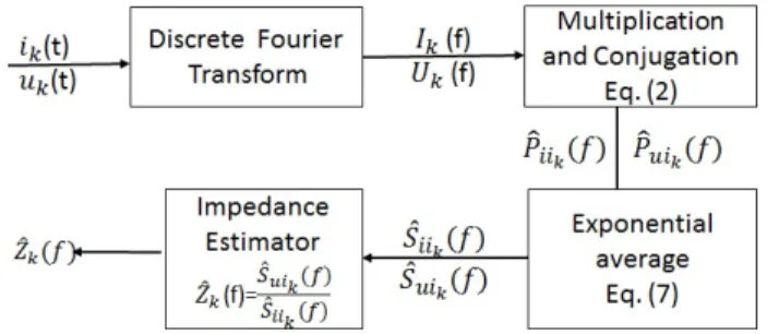
The whole algorithm used to recursively estimate Z(f) is briefly described in Fig. 2. This algorithm leads to an updated estimation ˆZk(f) of the battery impedance at
each new block of data, allowing to follow the variations of the impedance over time.
Figure 2: Recursive wideband frequency estimation algorithm.
From Eq. (7), it is clear that when a = 0, no average is performed and then
Zk(f) = UIk(f )
k(f ). In that case, the battery impedance is simply estimated by the ratio
of the Fourier transforms of the voltage and the current, leading to poor estimation performance regarding measurement noise. When a increases, the power spectral densities involved in the impedance estimation are more and more averaged, and the final estimator tends to the result obtained in the non-recursive case when a → 1.
2.4 Comparison of the three methods
a) Nature of the estimation
In the rest of this paper, we compare the estimation performance of three estimation methods presented previously:
• the classical GEIS,
• the non recursive version of the estimation algorithm given in Eq. (2), (3), and (4),
• the recursive version of this algorithm described in Fig.2.
It must be noticed that the two first methods lead to only one estimation of the impedance, while the last method gives access to several estimates continuously updated all along the measurement process. In that sense, impedances estimated with the GEIS and the non-recursive algorithm are similar to a snapshot of the state of the battery, while the one obtained with the recursive algorithm is able to track the temporal variations of the true battery impedance.
b) Estimation error
A performance indicator quantifying the estimation quality reached by the considered algorithms is clearly needed. A natural and simple indicator is the normalized root-mean-square error between a known reference value of the impedance Zref(f) and
the kth estimated value of this impedance Z
k(f). Eq. (8) defines this quantity,
expressed in percent, over a frequency band B. RMSEk= 100 s P f ∈B|Zref(f) − ˆZk(f)| 2 P f ∈B|Zref(f)| 2 (8)
Obviously if this indicator equals zero, the algorithm perfectly estimates the battery impedance over the chosen frequency band B since then ˆZk(f) = Zref(f), ∀f ∈ B.
3. Experimental results
The goal of this part is to compare experimentally the estimation performance of the proposed and usual methods. This comparison is conducted on a commercial lithium nickel manganese cobalt oxyde (NMC)/ Graphite battery with a nominal capacity C of 2.2 Ah (discharge at 25 °C, 2 C, Umin = 2.7 V). The frequency band on which the electrical impedance of this battery is estimated is 20 Hz - 90 Hz.
3.1 Experimental protocol
a) Charge and discharge
The battery was placed in an enclosure with controlled temperature of 25 °C. After a complete charge (25 °C, constant current of C/2 until 4.2 V, constant voltage during 1 h), we discharged the battery at a current of -0.5 A which corresponds
to a C-rate of C
4.4. In order to compare the estimates obtained by the wide-band
frequency algorithm with a known reference result, Zref(f) is first obtained thanks
to an impedance spectroscopy performed by the EC-Lab software associated with a VMP3 of Bio-Logic SAS. Therefore, once 10% of SOC is discharged, we first record a classical GEIS (signal amplitude of 200 mA, 3 measures, 1 Hz to 1 kHz, logarithm spacing of 10 measures per decade). Then we consecutively apply the same block of PRBS current centered around -0.5 A in order to apply the recursive and non recursive estimation algorithms and compare the obtained results.
b) Input current filtering
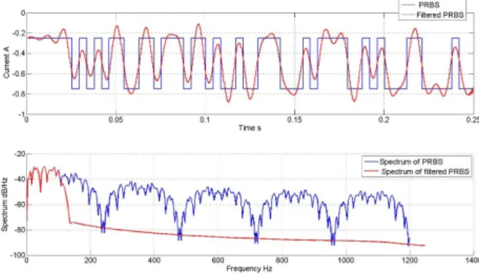
The block of PRBS current of length 0.25 s and amplitude of ± 250 mA is previously filtered thanks to a low-pass filter with a cutoff frequency of 120 Hz, higher than the maximum frequency for which the impedance must be estimated. Fig. 3 shows the temporal signals and their corresponding spectra.
Figure 3: One block of current signal (top: temporal signals; bottom: spectra). This filtered block is then repeated consecutively 36 times, leading to a measurement process with a total duration of 9 s. During this process, the current and the voltage of the battery are synchronously sampled at a sampling rate of 2500 Hz.
c) LTI assumption
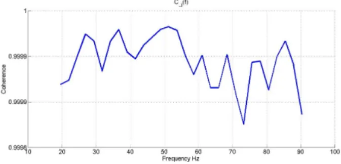
During the whole measurement process, the SOC evolution is lower than 1% leading to the assumption that the battery can be considered as linear and time-invariant. This important assumption can be confirmed thanks to the magnitude squared spectral coherence defined in the previous section. Fig. 4 shows that the magnitude squared spectral coherence stays close to 1 in the frequency band of interest. Indeed for all these frequencies the coherence is always above 0.9998.
This high value confirms that during one estimation process, the battery behaves as a LTI system and its electrical impedance can be theoretically defined by Eq. (1) and estimated with Eq. (4).
Figure 4: Magnitude squared spectral coherence estimated between 20 Hz and 90 Hz during one estimation process.
3.2 Estimation results
a) Impedance estimation for a SOC of 90%
Fig. 5 shows the results obtained with a forgetting factor a = 0.9. We can notice on the Nyquist plots that the non-recursive estimation is close to the estimation obtained through the usual GEIS, and that the recursive method seems less accurate. This can be explained by the time window over which each estimator is averaged. The non-recursive estimate is averaged over the whole data set leading to good estimation performance. On the contrary, the non-recursive estimate is averaged over a smaller local window whose size is set by using the forgetting factor a (the closer to 1 a is, the longer the time window is).
Figure 5: Estimated impedances between 20 Hz to 90 Hz by using the three methods. The learning curves shown in Fig. 6 represent the time evolution of the estimation performance indicator defined in Eq. (8) in the recursive (red curve) and non-recursive (green curve) cases. As expected, the error for the non-non-recursive algorithm is always lower than the one obtained in the recursive case. Moreover two steps are clearly visible on the red learning curve: a first decaying part corresponding to the convergence time of the algorithm (duration = 2.5 s), and a second part after convergence where the estimate fluctuates around the correct impedance.
Figure 6: Learning curves (time evolution of the root-mean-square error).
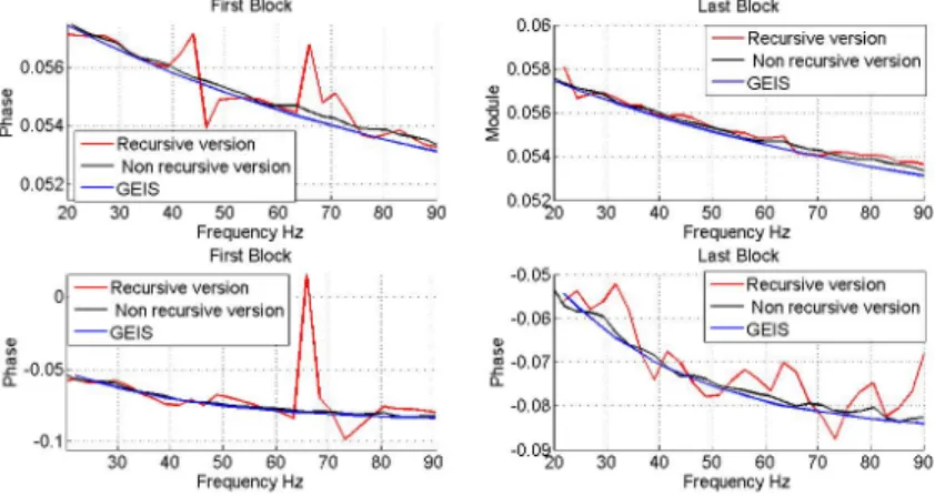
Figure 7: Difference between first and last estimation for the recursive case (left: 1stestimation, right: last estimation; top: module, bottom: phase).
Fig. 7 highlights the difference of estimation accuracy between first and last temporal estimates of the battery impedance (both module and phase are represented). Once the convergent step of the recursive algorithm is finished, the estimation performance becomes clearly more accurate, explaining the large decrease in the learning curves of Fig. 6.
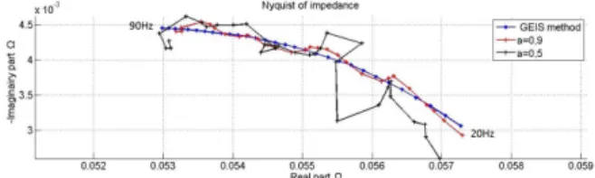
b) Influence of the forgetting factor
The parameter which controls the length of the convergence time and the quantity of fluctuations around the final error is the forgetting factor a. Fig. 8 and 9 highlight the influence of this parameter on the estimated impedance (Nyquist diagrams in Fig. 8) and on the learning curve of the algorithm (Fig. 9). For a forgetting factor close to 1 (a = 0.9, red curves), a large convergence time is obtained (around 2.5 s) with small final estimation error and fluctuations. For a smaller forgetting factor (a = 0.5, black curves), the convergence time is much shorter (around 1 s) but the
Figure 8: Nyquist diagram for a = 0.9 (red), a = 0.5 (black), and the GEIS method (blue).
Figure 9: Learning curves for a = 0.5 (black), a = 0.9 (red), and the non-recursive algorithm (green).
These results highlight the existence of a trade-off between the obtained convergence time (related to the tracking capabilities of the algorithm) and the final estimation error (related to the estimation performance of the algorithm). This trade-off can be managed through the value of the forgetting factor a. Indeed, a small forgetting fac-tor leads to an algorithm able to follow strong variations of the estimated impedance over time, but with a large estimation error. On the contrary, a forgetting factor close to 1 leads to an algorithm able to precisely estimate the battery impedance, but unable to follow large time variations.
c) Algorithm complexity
Several criteria can be used to further refine the comparison between the three considered methods. For example, their software complexity and their computation time can be analyzed. In our case, we measured that for the frequency band used in this paper (20 Hz - 90 Hz) the recursive algorithm only needs 0.25 s to be updated, while the other methods require 3 s. The electronic circuitry needed to implement the methods is also of interest for embedded systems. Concerning wideband frequency estimation methods, the input current signal is a low-pass filtered PRBS that can be simply generated by using an electronic switch (such as a transistor) followed by an analog low-pass filter, while a more complex system generating sine waves with different frequencies is needed in the GEIS case.
4. Conclusion
To conclude, the proposed recursive algorithm allows a continuous tracking of battery impedances. The trade-off between its convergence time and its final estimation error is controlled by the value of the forgetting factor: the closer to 1 this parameter is, the longer the convergence time is and the lower the final estimation error and its fluctuations are. Moreover, wideband methods seem to be much simpler and cheaper to embed than a usual GEIS strategy. In the near future, this algorithm will be implemented in an embedded system and applied to a test bench in real-time.
Bibliography
[1] F. Huet, “A review of impedance measurements for determination of the state-of-charge or state-of-health of secondary batteries,” Journal of
Power Sources 70, pp. 59–69, 1998.
[2] O.S.Bohen, “Impedance-based battery monitoring,” Institute for Power Electronics and Electrical Drives RWTH Aachen University, 2008. [3] U. Tröltzsch, O. Kanoun, and H-R.Tränkler, “Characterizing aging effects
of lithium ion batteries by impedance spectroscopy,” Electrochimica Acta
51, pp. 1664–11 672, 2006.
[4] E. Barsoukov and J. R. Macdonald, Impedance Spectroscopy Theory,
Experiment, and Applications. 2005.
[5] R. Pintelon and J. Schoukens, System Identification, a frequency domain
approach. 2004.
[6] R.Al-Nazer, V. Cattin, and P. Granjon, “Broadband identification of battery electrical impedance for hevs,” IEEE Transactions on Vehicular
Technology 62 n. 7, pp. 2896–2905, 2013.
[7] P.-D. Welch, “The use of fast fourier transform for the estimation of power spectra: a method based on time averaging over short, modified periodograms,” IEEE Trans. on Audio Electroacoustics, Vol. AU-15, pp. 70–73, 1967.
[8] J. S. Bendat and A. G. Piersol, Random Data: Analysis and Measurement