HAL Id: in2p3-00019962
http://hal.in2p3.fr/in2p3-00019962
Submitted on 23 Apr 2009
HAL is a multi-disciplinary open access
archive for the deposit and dissemination of
sci-entific research documents, whether they are
pub-lished or not. The documents may come from
teaching and research institutions in France or
abroad, or from public or private research centers.
L’archive ouverte pluridisciplinaire HAL, est
destinée au dépôt et à la diffusion de documents
scientifiques de niveau recherche, publiés ou non,
émanant des établissements d’enseignement et de
recherche français ou étrangers, des laboratoires
publics ou privés.
Phase transitions in finite systems
P. Chomaz, F. Gulminelli
To cite this version:
... ... ... .... .. ...
R0203260
....
.. ..
.... . ....
..
. . ...
..
XX X xX
...
...
.. ... ...
.. ... ...
. ... ...
. . ...
... ..I
...
... ... .
... ... ... ..
... ... .
.
. ... ...
... ... ... ... ...
...
. .. ....
...
.. . ...
...
...
...
... ...
... .. ...
...
... ... ...
.. .. .. .. ...
... ...
x
: ... .. .
...
... ...
...
... ... ....
...
...
...
... .
... ..
... .
...
....
....
...
...
...
xxxxxx]:x:
x]
... .. ... ...
.... ..
.. ...
....
.. ..
...
...
.. . ... ... .
... .. ..
...
....
....
...
...
. ...
. .. .. ...
. ...
...
...
. . .. .
...
.... .
... ... ... ...
.. ....
...
.. ... ....
.
....
....
....
...
...
...
...
.... ...
. ...
.. ....
.. ...
.. . . ... ...
. ... .
...
...
... .
... ...
...
...
...
. .
... ...
...
... .
...
. . .
... ...
....
...
...
.. .. . ....
.... ...
.
....
...
...
..
... ....
... ... ... ..
...
...
... .. ...
...
... ... ... .
... .... ... ... ..
...
...
... ... .
... ...
... .
...
.. ....
.... ...
...
... .
.... .. ..
....
. .... ....
... .. .. ...
... ... ... .. ....
...
.. .... ... .. ... .
.. .. ... ... ...
.. ...
... ... ...
...
...
.. .... ... ....
.. .. ....
.. ... ...
... ...
... ..
...
... ...
... .. .
....
....
....
....
....
....
....
...
...
...
...
...
...
... ...
... ..
...
.... ..
... .. ..
.... .... ..
.... ..
... ...
... .. . .... ...
... ... .... .
... .... .]]:
. . . .
...
... ... ...
... .. .
.. ... ....
.. .... .
....
....
....
....
...
...
... ....
... . ...
...
... .. ....
. . ...
. . ...
...
...
... I...
...
.. ... ... ..
... ...
...
.. ... .
... .. ... ... ... .. .
...
...
....
...
...
...
... ..
...
... ... ..
...
...: ...
...
.. . . ... .. .... .
... .. ... .... ...
... .. ...
. ... .. .. ..
...
... ... ...
... ..
... .
.. ... ...
...
...
....
.. ... ..
...
...
...
.. ..
....
.... ... ... ... ... .. ... ..
.... ....
.. ... ... ... ....
.... ...
...
..
.... .... ...
...
...
...
... ... .. .
....
.. ...
.. .... ...
... .
... ...
...
....
....
... .... ...
.. ...
... ....
...
...
...
...
...
...
...
....
...
... .... ... .. .... ....
...
... ... ....
....
... .... .... .
... ..
....
...
... ... ..
... ...
....
... ... ... ...
... ...
... ...
...
...
....
....
... ... .. .. .. ..
... .. ... ....
..
... ...
...
...
... .. ....
... .... ... .... ...
... ....
... .. .
...
...
... ... .. ... .. ....
....
...
... ... .... ... ....
..
. ... .. ... ..
...
... .. .. ..
... ...
.... ... ..
.. ... ... .. .... ....
...
. .. .
...
... ...
.. ... ... ...
...
....
.
... ...
... ..
.
...
.. ...
... ... ...
... ...
...
...
...
... ... ...
... .... ... ..
. .... .
...
...
....
...
...
... ...
... ... ...
...
.. ... .. ..
.. .
...
.. ...
...
... ...
...
...
...
... ...
...
...
... ...
.... ... ...
... ... ... ... ...
...
...
. ... .. .. . ...
X
X
X
X
.... ...
... .... ...
... ...
...
..
....
.
...
...
...
...
... ...
.. ...
...
...
...
... ...
... .. ...
...
... .. ... ...
. ... ... .
. ....
...
. ...
. . .
. ...
... .. ..
.... .... ....
... . ....
...
...
... ....
...
....
....
...
.. ...
... ...
...
. .. . .. .
...
::
:
:
: :
.... ...
.
xxxxxx :::x ... ...
... .... . .
. .... ... ..
...
..
.... ...
.. ...
... ...
. ... ..
. . ....
....
..
... ..
x X
...
....
...
...
.. . ...
....
.... ...
... ...
xx
:
... .. ...
....
...
.... ...
...
... .. . .. .... ..
....
.. . . ..
...
...
...
...
... .
...
...
... ....
.... .. ... ..
.. ... ...
...
... ...
...
...
..
.... ... ...
...
....
..
. .. ... .
... ...
.. ...
...
...
....
... ... ... ....
. ..
... ...
...
...
. . ... ...
...
... ...
... ...
... ...
...
x
:x
x x x : : :::
:::
...
...
... . ..
...
...
....
..
...
. ...
...
....
... ... ...
.... ....
... I .... ... .
... ... . . .
... ..
... : : : : : : : : : ::: ... ... ... ...
...
...
. .. ... ... ... ... .
...
.
. ...
.
... ...
...
...
... .
. .. ... . ...
...
... .. ... ...
...
... ..
... ... ...
...
... ...
... ....
...
...
...
...
...
... ... ...
...
...
...
...
estio
...
...
. ...
D OO, I'Enreg.
.... ...
... ...
N 'TR N
r-Phase Transitions in finite systems
Ph. Chomazi and F. Gulminelli2
GANIL (DSM-CEA/IN2P3- MRS), B.P.50271 F-14021 Caen cedex, Rance ITC Caen, (IN2P3-CNRS/ISMRA et UniversiW). F-14050 Caen cedex, France
... ... ... ... ... ... ... ... .... ...... ... .. ... ...... ... ... ...... ......... ... ... ... ... ... ... ... ... ... ... ... .. ... ..... ... .. ... . ... .... .. ...... ... ... ... ... ... ... .... ... ... ... .. .... ...... ... ... .. ... ...... ... ... ... ... ... ... ... .... .... ..... ...... .... ......... ........ ... ...... .. ... ....... .... ... ... ..... .. ... ... ... ... ... .... .. ... ... ..... ... .. ... .... ......... ... ........ .. ... ... ... .... ... .... ... ...... ... . . .. ... .. . .. ... ... .. .. . ... .... . ....... ... ....... ... ... . . . . .. ... ... .... .. ... ... .. ... ... ... ... . .... .... ... .... .... .. . ... ... .. .... . . ... .... ... ... ... ... .. .. ...X . ... ... .. ... ... ... ... ... ... X : ... .... ... .. .... .... ...... .. ... .. ... ... ... ... . .. ... ... ... ... ... ... .. ... . ... .. .... . . . .. .. .... .. ... ... ... ... ... ... ... . ... . ....
GANIL P 02 16
...
i
Ph. Chomazi and F. Gulminelli2
1 GANIL (DSM-CEA/IN2P3-CNRS), B.P.5027 F14021 Caen cedex, France 2 LPC Caen, (IN2P3-CNRS/ISMRA et Universit6) F14050 Caen cedex, France
Abstract. In this series of lectures we will first review the general theory of phase tran-sition in the framework of information theory and briefly address some of the well known mean field solutions of three dimensional problems. The theory of phase transitions in finite systems will then be discussed, with a special emphasis to the conceptual problems linked to a thermodynamical description for small, short-lived, open systems as metal clusters and data samples coming from nuclear collisions. The concept of negative heat capacity developed in the early seventies in the context of self-gravitating systems will be reinterpreted in the general framework of convexity anomalies of thermostatistical po-tentials. The connection with the distribution of the order parameter will lead us to a definition of first order phase transitions in finite systems based on topology anomalies of the event distribution in the space of observations. Finally a careful study of the ther-modynarnical limit will provide a bridge with the standard theory of phase transitions and show that in a wide class of physical situations the different statistical ensembles are irreducibly inequivalent.
1
Equilibrium and Information
1.1 States and observables 23]
Modern physics associates to every physical system two different types of o-jects: observables that characterize the measurable physical quantities and states
whose knowledge allows to predict the result of experiments. From the mi-croscopic point of view, single realizations of systems with N degrees of free-dom are characterized by a pure state (or microstate), that is a wave function,
ITIN), in quantum mechanics or a point in the 2N-dimensional phase space,
s = qjq2,...,qN;P1,P2,.--1pN), with qj and pi the position and momentum of
each degree of freedom, in classical mechanics. If systems are sufficiently com-plex, the exact state is in general impossible to define and each actual realization corresponds to a microstate (n) with the probability p('). In such a realistic case, one rather speaks of mixed states (or macrostates) described the density
1: 10(n)) (n) ,p(n) I
or b (s = E 6 (s - s('))n
n
Observables are operators defined on the Hilbert space or classically real functions of 2N real variables. The information that can be associated to the system is the ensemble of expectation values of the observables .1i, on the
2 Ph. Chomaz and F. Gulminelli
state. i.e. the ensemble of observations
(11
= E'p
AW where A(") is theI
I
actual result of a measurement on the realization (n). In the quantum case (, = pn) (0(n) 1.,, 1,(n) = Tr (bj,). Both for pure and mixed states, if the information on the system is complete at the initial time, this stays true at any time because the dynamical evolution of states is governed by the de-terministic Liouville Von Neumann
equation at
= ft' bj
where ft is the Hamiltonian of the system and where f.,.j is the commutator divided by ih in quantum mechanics which reduces to the usual Poisson bracket at the classical limit. However in the case of complex systems, the initial conditions are in gen-eral incompletely known and an exact solution of the Liouville Von Neumann equation is out of reach. In general only a small set of pertinent observables is known at any time which is sufficient to determine the state (i.e. the totality of the p(n)) because of the complexity of the density operator.1.2 The Shannon entropy[2,3]
The incompleteness of the available information can be measured through the lack of information or statistical entropy
= E
P(-) In P(n = -Tr (b In b)n
Let us show within a simple example that the statistical entropy (or Shannon entropy) indeed measures the lack of information.
Let us consider a system constituted of N identical boxes and an experiment consisting in putting randomly a ball in a box. The missing information to know where the ball is depends first on the occupation probability of each box
= Sp(l)'...' p(N)). Let us first consider equiprobable boxes p(' = 11N, Vn.
In this case depends only on the total number of boxes, = S(N).
Let us enumerate some ftmdamental properties of
The lack of information must grow with the number of possible results
S(Ni > S(N2) V N > N2.
Let us divide the N boxes into N, groups of N2 boxes each, N = NN2. The experiment now consists in two successive steps, first find out in which group out of the N equiprobable ones the ball is (which is associated to a lack of information S(NI) ) and then determine which of the N2 equiprobable boxes belonging to the group the ball is (associated to a lack of information S(N2)).
The missing information of the two steps experiment is then S(Ni) + S(N2).
The information cannot depend on the number of steps through which it is collected S (N = S(N -N2 = S(Ni) + S(N2).
The ensemble of these properties is fulfilled by a logarithmic function S(N) k In N where k is a constant.
We have just shown that the Shannon entropy coincides for equiprobable states with the Boltzmann entropy (or microcanonical entropy). Let us now turn to the more general case in which boxes are not equiprobable. To derive the associated information let us consider a big number W (eventually going to infinity) of experiments identical to the one described above. Among these W experiences, a number N : WIN will lead to the observation of the ball in the i-th box. This experimental result defines a osterioH a probability pi = N1W for the i-th box.
Within this result fNi,..., Nk,..., N1vJ, the number of possible configurations for the box is given by the combinatorial
W! (W - N,)! W!
N,! (W - N,)! N2! (W - N - N2)! Ili Ni!
where the first term represents the number of ways of choosing N, indistinguish-able objects out of W, and so on. All the events are equiprobable. The entropy is then
S(S? = k In S = k (n W - In Ni!)
= k(W In W - W - E(Ni In N - N))
= k(W In W - E(Wpi In W + Wpi Inpi))
i
- -kW
E
pi In pii
where we have used the Stirling formula InN! z NInN - N. The additiv-ity property introduced above allows to conclude that for a single experiment the missing information is given by the Shannon entropy S(p(,),...,P (N) - k E,, p0n) In p(-).
It may be interesting to know that if the additivity property of the infor-mation is relaxed, it is possible to construct a non-extensive extension of the Shannon theory based on the so called q-statistics which has interesting applica-tions in out of equilibrium situaapplica-tions as in the case of turbulent flows 4 In the following of these lectures we will limit ourselves to the standard information kernel introduced above.
1.3 The fundamental postulate of statistical mechanics
The fundamental postulate of statistical mechanics can be expressed as follows "The statistical distribution of microstates usually called the equilibrium is the one which maximizes the statistical entropy within the external constraints
4 Ph. Chomaz and F ulmineffi
Indeed any other distribution would introduce an extra piece of information, in contrast with the statement that all the available information is given by the constraint.
It is important to remark that this postulate, though certainly intuitive and elegant. does not necessarily imply that the theory has any predictive power: the fact that we have only a limited amount of information on a system does not necessarily mean that the information contained in the system is objectively limited. In this series of lectures we shall anyway keep the fundamental postulate as the only reasonable working hypothesis in a complex system.
The fundamental postulate of statistical mechanics allows to determine the equilibrium values of the state probabilities p(l). This task is easily accomplished with the help of the method of Lagrange multipliers.
1.4 The method of Lagrange multipliers[5]
Let us consider the problem of finding an extremurn of a two variables real function f (x, y) along a curve defined by the relation w(x, y = wo. To this aim the standard way is to calculate the total differential
d = af dx + af dy
Ox ay
where dx and dy are linked by the relation
&'J aw dx + aw dy =
ax
ay
Expressing dy as a function of dx the differential reads
d = af - aw'ax of )dx
Ox
awlOy
Putting df to zero at the point (xO, yo) which fulfills the constraint w(xo, yo)
wo, leads to
aw
f J-O'Y = w af J.01YO
ay
axax ay
which defines the coordinates xO, yo) of the extremurn.This same result can be obtained in a simpler way if we introduce a Lagrange multiplier A and we define the auxiliary function F = f - A(w -wo) that coincides with the function f on the curve we are interested in. Differentiating F respect to its two independent variables x and y
Of
dF = -A aw )dx + (af - Aau' )dy
ax
ax
ay
ay
the two partial derivatives have to go to zero separately at the extremum leading to a solution (xO (A), yo (A)). This extrernum fulfills the condition
aw af J-.'YO aw Of J-01YO
ay ax
09 ay
which exactly corresponds to the condition above if A is such that w(xo (A), yo (A)) = wo. The extension to a bigger number of variables and constraints is straightforward.
To summarize, this method allows to replace the study of a function of non independent variables to the study of an auxiliary function for which all variables are independent and the constraints are absorbed by real numbers (Lagrange multipliers).
1.5 The equilibrium [5]
Let us use this method to maximize the statistical entropy = Tr15 n 15 under the constraint of a given set of L observations 01)
This situation corresponds to the L constraints TrbA = A, that has to be augmented with the extra constraint of the normalization of probability R15 which can be incorporated as an additional observable Ao = 1. The auxiliary function is defined as
L
= Trb in b
E
\jTrbAj1=0
The variation of Y induced by a variation bb of the density matrix reads
L
by = -T-6b In b I
E
AA,The extremum correspond to by 0, with no restrictions on 6b leading to the condition In b I 0 AiA = 0. The solution is the density matrix at
equilibrium which is a function of the Lagrange multipliers Al
bo = 1
- exp AA, (2)
Z
where we have already taken care of the normalization constraint by introducing the partition sum
L
6 Ph. Chomaz and F. Gulminelli
The link between a constraint
01)
(or observation, or extensive variable) and the associated Lagrange multiplier Al(or thermodynamically conjugated inten-sive variable) is given by an equation of statealnZ (4)
aAl
It is also possible to express Al as a function of A) by inverting the equation of state. Indeed the equilibrium corresponding to the considered constraints is associated to a value for the statistical entropy
= rbo In bo Al A,) + InZ (5)
This last equation known as a Legendre transform gives the relation between the entropy and the partition sum and implies for the Lagrange multipliers
Al =
as
(6)a(A,
It should be noticed that while Do and Z are functions of the intensive variables (Al), the Legendre transform is a function of the associated extensive variables Ai).
Using es.(2,3,4) te whole thermodynamics of the system can be calculated if the constraints A,) are known. It is important to remark that this formalism is completely general in the sense that it can be applied for an arbitrary number of bodies with no need of a thermodynamical limit (infinite systems), and that all observables (and not only variables conserved by the dynamics) can play the role of constraints. Moreover the maximization of entropy as a tool to deal with the general problem of missing information can be extended in dynamical situations and has shown to be a fruitful approach in the field of stochastic quantum transport [6]_
1.6 The usual thermodynamics [5]
The usual ensembles of standard thermodynamics can also be obtained as ap-plications of this general theory. Let us consider for example the case where the only constraint is the energy E = Tr (boft = EpE(n) associated with the Lagrange multiplier 3 The probability of the n-th energy eigenstate is then po = 1 exp(-OE(n)) while the energy probability distribution reads
n -20
p,3(E = W(E) exp(-,8E) where W(E) is the number of states corresponding toZO
an energy E. The Lagrange multiplier has the physical meaning of the inverse of the temperature T = -1. The relation between the average energy and the
temperature is given by the equation of state (E = -a,3 In ZO and the Legendre transform S ((E)) = In Z,3 + 0 E) represents the well known relation between the canonical entropy and the free energy FT = 0-' In Z,3.
The microcanonical ensemble can also be obtained from this general theory considering that in the absence of any constraint (except the normalization of probabilities) all states must be equiprobable. The microcanonical entropy is then obtained as the expression of the Shannon entropy within the equilibrium distribution p = 11W(E), S(E) Z EW1 W` In W` i= = In W.
2 Generalities about phase transitions
Generally speaking, for a given value of the control parameters (or intensive variables) Al, the properties of a substance are univocally defined, i.e. the con-jugated extensive variables 01) have a unique value unambiguously defined by the corresponding equation of state For instance the volume occupied by n moles of an ideal gas at a given pressure P and temperature T is given by V = nRTIP . In reality we have seen in the previous chapter that extensive variables, being by definition expectation values of operators, are associated with a probability distribution unless the system is described by a pure state. The intuitive expectation that extensive variables at equilibrium have a unique value therefore means that the probability distribution is narrow and normal, such that a good approximation can be obtained by replacing the distribution with its most probable value.
In this case, as we will see in section 21, the Legendre transform gives an exact mapping between the standard intensive ensembles in which the control parameter is intensive or equivalently only the average of the extensive variable is known and the more exotic extensive ensembles where an extensive variable is controlled event by event, demonstrating the equivalence between the different statistical ensembles. In the following we will often take as an paradigm of inten-sive ensembles the canonical ensemble for which the inverse of the temperature O' (or equivalently the average energy (E) is controlled while the archetype of the extensive ensemble will be the microcanonical one for which the energy is strictly controlled.
The normality of probability distributions is usually assumed on the basis of the central limit theorem that we will briefly review in section 22. However some situations exist in which the probability distributions of extensive variables are abnormal and for example bimodal: in this case two different properties (phase$) coexist for the same value of the intensive control variable. A first elementary description of phase coexistence using this intuitive bimodality argument will be given at the end of section 22.
The topological anomalies of probability distributions and the failure of the central limit theorem in phase coexistence imply that in a first order phase transition the different statistical ensembles ae in general not equivalent and different phenomena can be observed depending on the fact that the controlled variable is extensive or intensive. This general statement will be developed in
8 Ph. Chomaz and F Gulminelli
great detail in chapter 4 and its far reaching consequences will be analyzed in chapter 6.
2.1 The difference between Laplace and Legendre,
We have seen in the last chapter that the relation between the different ther-mostatistical potentials is given by the Legendre transform. It is important to distinguish between transformations within the same statistical ensemble as the Legendre transform (which gives for instance the link between the canonical partition sum and the canonical entropy) and transformations between differ-ent ensembles wich are instead given by non linear integral transforms. Let us consider energy as the extensive observable and temperature as the conjugated intensive one. The definition of the canonical partition sum is
Ze = 1: exp(-OE("))
n
where the sum runs over the available eigenstates n of the Hamiltonian. If energy can be treated as a continuum variable this equation can be written as
00
ZO dE W(E) exp(-OE) (7)
which is nothing but a Laplace transform between the canonical partition sum and the microcanonical entropy SE = In W(E). If the integrand f (E = W(E) exp(-OE) is a strongly peaked function the integral can be replaced by the maximum f (f)
Z,3 zt; W(E) exp(-OE) (8)
which can be rewritten as
In ZO zz Sp - 3E (9)
or introducing the free energy F In Z,9
FT E - TS2
Eq.(9) has the structure of an approximate Legendre transform and shows that in the saddle point approximation eq.(8) the ensembles differing at the level of constraints acting on a specific observable (here energy) differ only by a simple linear transformation. We will see in the next section and in more details in chapter 6 that however the saddle point approximation eq.(8) can be highly incorrect close to a phase transition. In particular, when the canonical distribution of energy is bimodal a unique saddle point approximation becomes inadequate. In this case eq.(9) cannot be applied and eq.(7) is the only possible transformation between the different ensembles.
• the link between the thermodynamical potential of the intensive (e.g. log of canonical partition sum) and of the extensive ensemble (e.g. the microcanoni-cal entropy) which are always related with a Laplace transform. This Laplace transform may lead to an approximate Legendre transformation for normal distributions but we know that this Legendre transformation is wrong if the distribution is abnormal.
• with the exact Legendre transform between the entropy of the intensive ensemble and the corresponding thermodynamical potential.
This simply corresponds to the fact that the microcanonical and canonical entropies can be very different.
2.2 The central limit theorem and phase coexistence
The typical representation of the probability distribution of any generic random variable depending on a not too small number of degrees of freedom is a Gaussian distribution. The very general validity of the Gaussian is due to one of the most important theorems of statistics, the Laplace central limit theorem. Let us consider an extensive observable E (i.e., energy) that can be written as the sum of I independent contributions (i.e. the energy of the different particles constituting the system) E ei , where the ei follow an arbitrary probability distribution with the unique requirement that the global variance El((e? _ e
E i 't 'i)2)/l
is finite. Then the central limit theorem states that the distribution of E tends to a Gaussian distribution with a width decreasing with the number of degrees of freedom
lim (E = 2 1 (E - (E))2 (10) I-CO P "2,, exp(- 2o,2/1 )
According to the central limit theorem at the thermodynamical limit the distribution of an extensive variable p(E) tends to a -function, implying as we have mentioned at the beginning of the chapter that the properties of the system are univocally defined by the value of the intensive parameter that controls the asymptotic value of (E) through the appropriate equation of state. Moreover in most cases a few tens of particles are enough for the Gaussian approximation to be correct, meaning that the limit appearing in eq.(10 ) can be neglected in practical applications. Another consequence of the central limit theorem is that the Laplace transform becomes equivalent to a Legendre transform as we have discussed in the preceding section, leading to the equivalence of statistical ensembles.
However a situation can occur in which the probability distribution is bi-modal and never tends to a Gaussian. Such a situation is called a first order phase transition. This patent violation of the central limit theorem is due to the fact that phase transitions are associated to long range correlations and the independence hypothesis between the different degrees of freedom breaks down.
Let us illustrate the standard picture of phase coexistence within a simple ex-ample. Consider a molecular system in the canonical ensemble characterized by
10 Ph. Chomaz and F Gulmineffi
the free energy F = -T In Z = E - TS. As we have demonstrated in section .3 the maximization of the statistical entropy with the energy constraint is equiva-lent to the minimization of the free energy. At low temperature a minimization of F is approximately equivalent to a minimization of (E): the equilibrium state of the system will be given by a compact configuration (a crystal or a liquid) with free energy FL (A, V). On the other side at high temperature the mini-mization of F corresponds to a maximini-mization of the canonical entropy, which will be achieved by a disordered rarefied state (a gas phase) with free energy
FG(A, V). Phase coexistence means that at an intermediate temperature the
two free energy solutions are allowed giving for the total free energy
F (A, V = FL (AL, V) + FG (AG, VG)
where AL, YL (AG, VG) are the fractions of total number of molecules A and
volume V belonging to the ordered (disordered) phase
A=AL+AG V=VL+VG
The equilibrium sharing of A and V is given by the minimization of the free energy
aF c)FL aFG aF aFL aFG
= 0 = __ - =
aAL aAL aAG aVL aVL aVG
implying the equality for the intensive variables conjugated to the mass number and the volume, namely the chemical potential and the pressure
PL = PC ILL = AG
This procedure can be generalized to any statistical ensemble. If we consider for example the microcanonical ensemble, the absence of constraints means that the thermostatistical potential is directly the microcanonical entropy
S(A, E, V) = In W(A, E, V) S (AL, EL, VL) S (AG, EG, VG) (12) with the extra conservation law E EL + EG. The extremization of S respect to
V and A gives again the equality of the chemical potential and pressure for the two coexisting phases, while the derivative respect to the energy variable gives
T = TG
where we have defined the microcanonical temperature as T-1
=
aES in anal-ogy with the canonical Legendre transform = aE) So (the justification of thephysical meaning of aES as an inverse temperature is postponed to chapter 4_ Equilibrium between the two phases is characterized by the equality of the temperatures. On the other hand, the conjugated extensive variables are different in the two phases EL < EG. This means that at the transition temperature Tt = T = TG the energy is discontinuous at the phase transition (latent heat). To summarize, in this standard view first order phase transitions are charac-terized by
• the presence of two phases in contact
• a discontinuity in (one ore more) first order derivatives of the thermostatis-tical potential (energy, volume, mass number ... .
To obtain this result we have written the thermostatistical potential as a simple sum of the contributions of the two phases (eqs.(11,12)). This is true only if the free energy (or entropy) of the interface between the two phases is negligible, i.e. for large systems interacting through short range forces.
In the next sections we will illustrate this standard view of first order phase transitions within an exactly solvable model in one and two dimensions (section 2.3 24) and in three dimensions with the help of the mean field approximation (chapter 3.
The additivity hypothesis of the thermostatistical potential breaks down for finite systems and even in the thermodynamical limit if the forces are long ranged. The far reaching consequences of dropping this approximation will be developed in chapter 4.
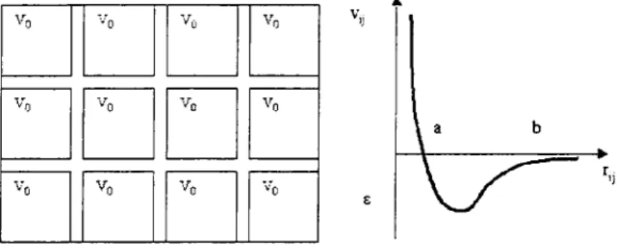
2.3 Isornorphism between Ising and Lattice Gas
Let us consider an ensemble of N classical spins which can take one of the two values Sk = ±1 on a lattice under the influence of an external magnetic field h and a constant coupling J between neighboring sites according to the Hamiltonian
N N
His = -h E Sk - - )7 Sk Si (13)
2
k=i kOi
where the second sum extends over closest neighbors.
The Ising model eq.(13) has been originally introduced to give a simple de-scription of ferromagnetism (i.e. a spontaneous magnetization that some sub-stances present in the absence of a field at low temperature). In reality the phenomenon of ferromagnetism is far too complicated to be treated in a satis-factory way by this oversimplified Hamiltonian; however the fact that the Ising model is exactly solvable in 1D and 2D and that very accurate numerical solu-tions exist for the three dimensional case makes this model a paradigm of first and second order phase transitions. The other appealing side of the Ising model is its versatility: introduced to explain magnetic phase transitions, it is also well adapted to describe fluid phase transitions. Indeed we can show that a close link exists between the Ising Hamiltonian eq.(13) and the Lattice Gas Hamiltonian which is the simplest modelization of the liquid-gas phase transition
I N 2 E N
HLG - Epknk - - E nknj (14) 2m k=1 2 kOi
In the Lattice Gas model, the same N lattice sites in D dimensions are characterized by an occupation nk = , 1 and by a D components momentum
12 Ph. Chomaz and F. Gulminelli
vector Pk- Occupied sites (particles) interact with a constant closest neighbor coupling .
Because of the transformation nk = (Sk 12 the Ising Hamiltonian HIS can be mapped into the interaction part H' of the Lattice Gas Hamiltonian
HLG. Indeed let us consider the interaction part of the Lattice Gas partition
sum in the grancanonical ensemble
7i-'=
E ...
-,3(Hj' - LA))LG
E
exp(ni=oi nN=Ol
where A = EN nk is the total number of particles and k , p are Lagrange multi-pliers. The factor multiplied by in the exponential can be written as
.'t E N Ez + 2p N Ez + 4p
HE - uA - - 1: SkS - 4 si - N 8
k*j
where z = 2D is the number of closest neighbors. With the identification J E/4 and h = ze + 2p) 4, this equation shows that the grancanonical partition sum of the Lattice Gas interaction hamiltonian is isomorphous to the canonical partition sum of the Ising model in an external field
,3 (H inl LC -,uA = OHI + K
where K is a constant. This result implies that all results obtained within the Ising model concerning magnetic transitions can be translated in terms of fluid transitions and vice-versa. In particular the magnetization m = Ek SO IN is related to the matter density p = Ck nk IN by m = - .
2.4 Exact solution of the Ising model in ID and D
The Ising model was proposed by Lenz to his student Ising in 1925. The exact solution of the model in one dimension is given in Ising's thesis.
Let us consider a one dimensional spin chain with periodic boundary condi-tions (spin ring). The Ising hamiltonian can be written as
N
His E (h5k + JkSk+l) k=1
and the partition sum results
1 1 N 1
ZIS
= E ... E
expOE
(hSk + JSkSki-1))E
712723 ... 7N1Sj=-1 5jV=-1 ( k=1 Sj=-1 SN=-l
h
7-ij = exp (Si Sj + SiSj
(2
If we consider the -j as the elements of a 2x2 matrix depending upon the two spins i and sj = ±
T T + r+
-'r- + T_
where the definition of the r j implies
,r + = exp,3(J + h) r - = exp O(J - h)
7- - = - + = exp(-OJ),
El
T2then we can write ,=-l rij7jk = k and the partition sum becomes
I N) N N I Q ) N) N
ZIS
= E
TjN =Tr (T A + Av = A Asl=-l 1 2 1 Al N oo 1
where Al, Al (Al > A2) are the eigenvalues of the T matrix The problem is then reduced to an eigenvalue problem
det (T - Al) = ; A 2 _ -r+ + + 7- A (-r +- -r -- =
After a little algebra we obtain the eigenvalues
2 A = exp(OJ) (ch(Oh ± (exp(-4,3J) + sh (h))'l
and the partition sum
2 2
In Zis = N OJ + In (ch(Oh) + (exp(-4,3J) + sh (Oh)) -1 ) )
It is easy to verify that In ZIS is a continuous function with continuous deriv-atives for all orders: the Ising model in one dimension does not present a phase transition. In particular the magnetization
1 a In ZIS 1 2 2
- - = sh(3h) (exp(-40J) + sh (h))'!
VO 9h 2
is a continuous monotonic function which is zero at zero field: no spontaneous magnetization is observed.
The solution of the Ising model in two dimensions[7] is far too complicated to be developed here. Let us simply give the asymptotic result N oo in the zero field case
14 Ph. Chomaz and F. Gulminelli M
AL T<T,
M A
T=Tc MAL T>Tc MOh
h
'0010/
h
-MO
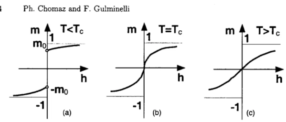
(a) (b) (C)Fig. 1. Schematic representation of the average magnetization as a unction of the applied
external field for the Ising model in more than one dimension at subcritical (left), critical (center) and supercritical (right) temperature.
Zis = 2ch (20J) exp 1)v (15)
1 = do In + ( - X2 sin2 2
27r 0 2
X 2 sh (20J) ch2 (20J)
With the partition sum of eq.(15) the magnetization equation of state can be computed. It is easy to verify that for temperatures lower than the critical temperature T = -' given by sh (2J,3, = the system presents a spontaneous magnetization at zero field[8]
mo = m(h = > = h2 (20J) (sh2 (20J) 1) 1/8 ___, (T - T) 1/8
sh4 (20J) 0 0C
The equation of state of the Ising model in more than one dimension is schematically shown in figure
At subcritical temperatures a discontinuity in magnetization is seen at zero field, showing that a first order phase transition is taking place in agreement with the intuitive arguments of the preceding section. For T = Tc the magnetization goes to zero as a power law (second order phase transition) while the equation of state is monotonous in the supercritical regime.
3
The mean field approximation
Even for simplified models such as Ising no analytical solution exists for a number of dimension D > 2 This is the reason why mean field solutions have been developed. The idea of the mean field approximation is to replace the intractable
N-body problem with an approximately equivalent analytical one body problem. Let us illustrate this method on the Ising case. If the Hamiltonian is composed of one body terms solely
N
Hlb
E
hkSk (16)k=1
with hk a generic one body operator, the thermodynamics of the system is solved in one line. Indeed the partition sum in the canonical ensemble reads
+1 +1 N
Zlb =
E ... E
exp (-OHlb = H Zk = exp (-Oh) exp (h) )N (17)$I= 1 SN= 1 k=1
where the last equality holds if hk = h Vk, and is promptly generalized to the
non-local case.
To reduce the Hamiltonian to a one body interaction the correlations among the different sites have to be neglected such that the interaction on a given site depends only of the coordinates of the site. This chapter is devoted to the applications of this approximation to the Ising model (section 31) and its general consequences for the problem of first order phase transitions (sections 32-3.3). We will see that an equivalent one body problem can be formulated and the two body character of the force results in a self-consistency problem for the equations of state which have to be solved iteratively.
It is important to stress that all mean field approaches are approximations which, because of the intrinsic lack of correlations., are especially bad in phase coexistence. In the recent years the enormous progress of computing machines has allowed the numerical solution of three dimensional models without any approximation with Monte-Carlo based methods. These exact solutions clearly show the inherent limitations of mean field approaches and will be discussed in chapter 4.
3.1 Mean field approximation for the Ising model
The interaction acting on the k-th site in the Ising model eq.(13) is hk = h +
J E, sj, where the sum extends over the first neighbors of site k A one body
term is obtained if the spin of the neighboring sites sj is assumed constant all over the lattice and equal to the average magnetization sj (s = m. In other
words the exact interaction is approximated by the interaction the site would experience if the spin distribution was uniform. The Ising Hamiltonian can then be written as a one body Hamiltonian
N N
HmF
hk$k+K=-T(h
+ JZM) Sk + K (18)16 Ph. Chomaz and F. Gulminelli
within a constant K which has to be determined by imposing that the expecta-tion value of HMF is equal to the mean field energy
EMF = -hNrn + Ein = N hrn + JZ M 2 (19)
MF 2
where the last equality is obtained by writing the interaction energy as
int -i -i ZM2
E = E 1: (Sk Si) - 1: 1: SO (Sj) J N
2 2 2
k=ljOk k=ljOk
which shows once again that the effect of the mean field approximation is the neglect of two body correlations. The comparison of eq. 19) with the expectation value of eq.(18) leads to the definition of the constant K as K = JNzm 2 /2 In fact this energy correction exactly compensates the double counting of the two-body interaction due to the introduction of the average interaction of each spin with all its neighbors. The mean field partition sum as for eq.(17) is factorized in the product of the individual partition sums of the different sites
ZMF =
E ... E
exp (-,3(HMF) = Z N (20)SI= ±1 SN=
where
Z exp, (-,3 (h + Jzm) s + JZrn2 2 exp 13 JZ M2) ch (O (h + Jzm))
2 2
which leads to a self-consistent equation for the magnetization
m = tanh (O (h + Jzm)) (21)
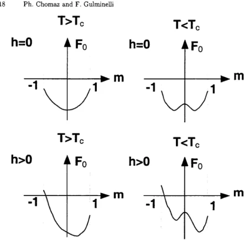
Equation 21) is represented in figure 2 in the subcritical, critical and su-percritical regime. If the behavior of the equation of state for T > T = Jz is qualitatively similar to the exact Onsager solution of section 24, in the first order phase transition regime the mean field solution shows a backbending behavior with a negative susceptibility X- = ahm region. To understand the physical meaning of the backbending, the free energy F = O' In ZMF is shown as a function of magnetization in figure 3 in the h = and h > case. From this figure one can see that the backbending corresponds to a maximum of the free energy, i.e. an instability. Indeed the coexistence between the two phases at dif-ferent magnetization cannot be obtained in a mean field calculation because of the intrinsic homogeneity hypothesis m = s) = const. The backbending there-fore reflects the instability of the homogeneous mean field solution with zero magnetization respect to the separation into two distinct phases at m = ± mo. At non zero field the magnetization oriented in the direction of the field has the minimum free energy, therefore will correspond to the unique equilibrium solu-tion. In the zero field case the two solutions have the same energy. This implies that every linear combination of these solutions
hAL
U
-MO
F_
'11/MO
MO
B
M
M
>Tc
>Tc
T=Tc
TC
TC
<Tc
Fig. 2 Left side: relation between the average magnetization and the magnetic field at
subcritical, critical and supercritical temperature for the three dimensional Ising model in
the mean field approximation. Right side: Maxwell construction modifying the subcritical
magnetization curve.
will have the same free energy; such a linear combination represents the
coex-istence between the two solutions as we have discussed in chapter 2 and
cor-responds to an horizontal straight line in the F - m and in the h - m plane
(tangent construction) as shown in the right part of figure 2
If the lack of correlations of the mean field is cured by allowing a mixed
phase according to eq. 22), the usual shape of the phase transition is recovered
(discontinuity in the first derivative of the thermodynamical potential).
To conclude this section we would like to comment the difference between
a self consistent approach as the mean field approximation and a genuine one
body Hamiltonian as in eq.(16),(17). We have shown in chapter
that the
thermodynamics of a system is completely determined once the partition sum
is known, since all thermodynamical quantities can be calculated as successive
derivatives of In Z . The Hamiltonian entering the mean field approximation of
the partition sum eq. 20) differs from the mean field approximation of the Ising
Hamiltonian because of the constant K which we have been forced to add for
the Hamiltonian to have the correct expectation value. The constant K in the
partition sum represents more than a trivial shift in the energy scale since K
depends on m which in turn is calculated from In Z showing the self-consistent
character of the approach. Following eqs.(16),(17) one could be tempted to define
from the mean field approximation to the Ising Hamiltonian a one body partition
sum as
N
Zib
( 1: exp (-O(h + Jzm)s)
S ±1
and the question arises weather thermostatistical observables can be obtained
from the successive derivatives Of Zib.
18 Ph. Chomaz and F. Guln-iinelli
T>T,
T<T,,
h=O
h=O
Fo
Fo
10. M
T>T,
T<T,,
h>O
Fo
h>O
Fo
M
M
Fig. 3 Mean field free energy as a function of magnetization at zero (upper part) and
positive (lower part) magnetic field, for a supercritical (left) and a subcritical (right) temperature.
To answer to this question one has to use the formalism of chapter and explicitly calculate the statistical entropy
SMF pi In pi
(pi (-OH(') - In
Zlb(Hlb) In Zlb
since the probability distribution for the mean field problem reads pi exp (-OH(") IZlb-The expectation of Hlb is readily calculated as
The general relation between entropy and free energy -F In ZMF
SMF - EMF finally leads to
In ZMF = In Zb + OE in, (24)
MF
Equation 24) shows that because of the two body interaction the partition sum is different from the one body partition sum even in the mean field approx-imation. In fact the difference comes from the double counting of the two-body interaction if the energy is calculated as (Hlb)
The best way to understand the mean-field approach is to consider mean-field solutions as a trial state to maximize the entropy completed by the constraints
(S -3 (E)) i.e. to variationally estimate the free energy F = -1 (S -3 (E)).
Then only the mean-field free energy can be considered as a good approximation of the exact free energy leading to,3F In Zlb - OEZ' which is nothing butF equation 24).
3.2 Implications for the liquid-gas transition
We have seen in section 23 that the isomorphism between the Ising model and the Lattice Gas model implies that all physical results concerning magnetic transitions can be easily translated in the fluid language and applied within minor modifications to the liquid-gas transition. To this aim the Ising canonical partition sum Z"', or free energy F = -O' In Z"', has to be transformed into the Lattice Gas grand-canonical partition sum ZGC or grand potential
S = -' In ZGC. If we only focus on the interaction part of the Lattice Gas model this leads to
exp (_O ( Uln) pAn,) exp, (-OSLG)
E
- LGn
(n) Zj
n
exp
(-O H N 2 NZj
exp (-OFls) exp 3N -
+
2 2
In the mean field approximation FIS
In
ZMFis given by eq. 20) giving
for the Lattice Gas grand potential
S?
i
2-' In (2ch (3 (h + Jzm)) - ZJ
ja
N 2 2 2
The total number of lattice sites in the Lattice Gas framework represents
the volume of the fluid N = V. The equation of state p
av In Z allows to
access the pressure
P= (Zj A jZM2)
+ -1 In (2ch ( (h + Jzm)))
(25)
V
2
-E ZP2
+ 0
In
1 P
20 Ph. Chomaz and F. Gulminelli
T>Tr,
=TC
Wb
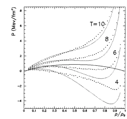
Fig.4. Isotherms in the pressure versus volume (in cell units b) plane for the three
di-mensional Lattice Gas model in the mean field approximation with a Mawell construction of the mixed phase. The coexistence zone is also indicated.
where the last equality is obtained using the magnetization equation of state eq.(21) and the substitutions m = 2p- 1, J = /2. Figure 4 shows some selected isotherms of the fluid equation of state. At subcritical temperatures T < T a clear backbending is seen reflecting the instability of the homogeneous mean field solution respect to the separation into distinct phases as in figure 2 above. Once again, if a linear interpolation of the liquid and gas volume solutions is imposed, the usual plateau of the Maxwell construction is recovered. The critical point is defined as the ending point of the coexistence zone, i.e. the point at which the first as well as the second derivative of the equation of state are zero. Substituting in eq. 25) we get p = 12, T = Jz, p = T, (In 2 - 12).
3.3 The Van der Waals equation of state
The Ising model in the mean field approximation reflects the same physics as the Van der Waals equation of state which describes a classical canonical gas of N identical molecules in an external pressure field po and volume V interacting via an attractive two body force. The free enthalpy connected to such a physical
scenario is
3
H = F oV = NT - bpN - TS + pV
Go
P
B
A
(a)
V
(b)
V
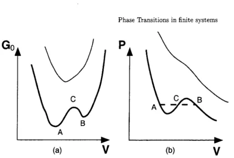
Fig. 5. Free energy and isotherms of the Van der Waals equation of state at a subcritical
and supercritical temperature.
Here p = NIV is the density of matter and bpN is the two body
interac-tion energy in the mean field approximainterac-tion. If we make an explicit use of the
equivalence between ensembles at the macroscopic limit, the entropy
can be
calculated in the mean field approximation as an effective one body problem
= In (WNWN)
V-Nvo
3
S = In W = ln(WWp)
r P= Nin
N
+ NInT
2
where the integral over the configuration space is
W
Nd
3,0(r3
_ V))NINI = (V - Nvc,)' INI
r
where vo is the volume occupied by each particle, the momentum space integral
gives
W
Nd'p exp(-p'/2,mT)
N = 27rmT)3N/2P
and we have used the Stirling approximation of the factorials. Using as above
the equation of state p = 0`0V In Z = ovF or the extremurn condition
L9V
= we get
NT
bN2
=
- -
(26)
V - Nvo
V
The free energy together with the isotherms are represented in figure 5. The
similarity with the microscopic results from the Ising model is evident. Once
again the volume interval
VA< V <
VBis unstable in the sense that if we mix
22 Ph. Chomaz and F. Culminelli
0
P/PC
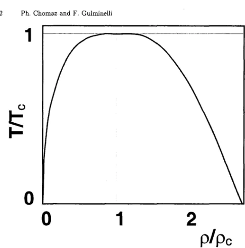
Fig. 6 Guggenheim's coexistence line in scaled variables obtained from many different
substances.
(H) does not change. This tangent construction is the well known equal area Maxwell construction since
VB VB
H(VB - H(VA = JVA dV dHldV = po (VB - VA) - 'VA dV p(V =
The coordinates of the critical point are found from dv pl = d' pl = V as V = 3NvO, T = 8b/27vo, p = b/27vo. If we introduce the scaled variables
= V/V = TITc, -x = p1p, one can readily verify that the Van der Waals
equation (26)becomes
8-r 3
7 = T-_--
--V 1 - 2
with no dependence on b or vo i.e. on the quantities specific of the structure of the gas.
This feature is preserved in realistic gases for which all thermodynamical variables can be rescaled according to the critical values leading to the famous Guggenheim phase diagram 9 (shown in figure 6 namely a unique coexistence
curve for many different substances which shows the universality character of phase transitions; this universality feature gives an a posteriori justification of the use of a schematic oversimplified model as the Ising model to describe complex and widely different physical phenomena.
3.4 The Landau Model
The simplest functional form of the thermodynamical potential as a function of the order parameter that contains all the physical situations discussed in the previous sections is given by
F(m = C + N (a(T)M2 + bM4 - hm) ; a T = ao (T - T) (27) where h is the intensive variable conjugated to the order parameter m. Note
b > in order to have a free energy bound from below in order to ensure that an absolute minimum (i.e. an equilibrium) does exist. Equation 27 is known in the literature as the result of Landau theory of phase transitions[10]. it is immediate to verify that in the proximity of the critical point T -- T, h + the order parameter and its derivatives follow a power law behavior m _+ IT, - T i
dm/dh --+ IT, - T where 12, -y = -1 are typical mean-field critical exponents.
Summarizing the present chapter, the mean field approximation leads to the definition of phase transitions as universal phenomena with the following characteristics
• presence of two different phases (i.e. minima of the thermodynamical poten-tial) that coexist in contact (via a non analyticity or tangent construction that mixes the two solutions in linear proportions)
• existence of critical points (or second order phase transitions) that corre-spond to the limit of the coexistence line
• definition of an order parameter (i.e. the extensive observable that allows to distinguish the two phases) that presents a discontinuity at the (first order) phase transition.
4
Finite systems: getting more from pushing less
In the preceding sections we have defined a first order phase transition as a dis-continuity in the first derivative (or order parameter) m of the thermodynamical potential F as a function of the control parameter. Such a discontinuity can exist only in the thermodynamical limit since
e this discontinuity corresponds to phase coexistence according to the equation (see section 22)
F(ce ml + ( - a) M2 = a F(ml) + (I - a) F(M2)
which holds if the free energy per particle is independent of the number of particles, i.e. if surface can be neglected respect to volume which is only possible if the volume goes to infinity.