Publisher’s version / Version de l'éditeur:
Journal of Infrastructure Systems, 19, 1, pp. 108-119, 2012-02-06
READ THESE TERMS AND CONDITIONS CAREFULLY BEFORE USING THIS WEBSITE.
https://nrc-publications.canada.ca/eng/copyright
Vous avez des questions? Nous pouvons vous aider. Pour communiquer directement avec un auteur, consultez la Questions? Contact the NRC Publications Archive team at
[email protected]. If you wish to email the authors directly, please see the first page of the publication for their contact information.
NRC Publications Archive
Archives des publications du CNRC
This publication could be one of several versions: author’s original, accepted manuscript or the publisher’s version. / La version de cette publication peut être l’une des suivantes : la version prépublication de l’auteur, la version acceptée du manuscrit ou la version de l’éditeur.
For the publisher’s version, please access the DOI link below./ Pour consulter la version de l’éditeur, utilisez le lien DOI ci-dessous.
https://doi.org/10.1061/(ASCE)IS.1943-555X.0000097
Access and use of this website and the material on it are subject to the Terms and Conditions set forth at
Performance of ductile iron pipes. I : characterization of external
corrosion patterns
Kleiner, Yehuda; Rajani, Balvant; Krys, Dennis
https://publications-cnrc.canada.ca/fra/droits
L’accès à ce site Web et l’utilisation de son contenu sont assujettis aux conditions présentées dans le site
LISEZ CES CONDITIONS ATTENTIVEMENT AVANT D’UTILISER CE SITE WEB.
NRC Publications Record / Notice d'Archives des publications de CNRC:
https://nrc-publications.canada.ca/eng/view/object/?id=4bf7116d-aa18-4a2c-9a0e-8b6def5a135c https://publications-cnrc.canada.ca/fra/voir/objet/?id=4bf7116d-aa18-4a2c-9a0e-8b6def5a135c
Performance of ductile iron pipes: characterization of external corrosion patterns
Yehuda Kleiner, Balvant Rajani and Dennis Krys
National Research Council of Canada, Institute for Research in Construction 1200 Montreal Road, Ottawa, Ontario K1A 0R6, Canada
Abstract:
Ductile iron pipes have been used in North America since the late 1950s. This paper, the first of two companion papers describes research that endeavored to gain a thorough understanding of the geometry of external corrosion pits and the factors (e.g., soil properties, appurtenances, service connections, etc.) that influence this geometry. This understanding is subsequently used in the second paper to devise a sampling scheme and to infer pipe condition of ductile iron buried water mains.
Soil corrosivity is not a directly measurable parameter and pipe external corrosion is largely a random phenomenon. The literature is replete with methods and systems that attempt to use soil properties (e.g., resistivity, pH, redox potential and others) to quantify soil corrosivity and subsequently predict pipe corrosion. In this research, varying lengths of ductile iron pipes were exhumed by several North American water utilities. The exhumed pipes were cut into short sections, sandblasted and tagged. Soil samples were also obtained at discrete locations along the exhumed pipe. Pipe sections were scanned for external corrosion using a specially developed laser scanner. Scanned corrosion data were processed using specially developed software to obtain information on pit-depth, pit-area and pit-volume. Statistical analyses were subsequently performed on these three geometrical attributes. Various soil characteristics were investigated to determine their impact on the geometric properties of the corrosion pits. Subsequently, a method is proposed to assess the condition of a ductile iron pipe, based on the geometry of corrosion pits of a few samples extracted along the pipe.
This paper, the first of two companion papers, describes the pipe exhumation, data preparation and statistical analysis of corrosion pits. The second paper describes a sampling scheme to infer pipe condition of a ductile iron buried water mains.
Introduction
Soil corrosivity is not a directly measurable parameter and the external corrosion of metallic pipes is largely a random phenomenon, hence, no explicit relationships exist between soil corrosivity and soil properties such as electrical resistivity, pH, redox potential, sulfate and chloride concentrations, moisture condition, shrink/swell properties and others. Moreover, no explicit relationship exists also between soil corrosivity and pipe deterioration rate. Virtually all the models in the literature that endeavor to propose such relationships are empirical. These models can generally be divided into two classes, namely, practical and empirical/probabilistic. The most widely known practical approach is the 10-point scoring method proposed by AWWA (Appendix A of ANSI/AWWA C105/A21.5-99), which classifies a soil as
corrosive/noncorrosive based on the weighted aggregation of 5 soil properties. The 25-point scoring method of Spickelmire (2002) is similar to the AWWA 10-point method except that other additional factors are included. As the 10-point method yields a binary response (corrosive/noncorrosive), some attempts have been made to fine-tune it using soft computing techniques, e.g., Sadiq et al. (2004) and Najjaran et al. (2006).
The work of several researchers, who have investigated the use of statistical/probabilistic tools to characterize the properties of corrosion pits, is briefly reviewed here. Aziz (1956) was among the first to use extreme value statistics (EVS), albeit not specifically for pipes but for aluminum samples immersed in water. His main conclusions were: (a) during the initial short period of exposure a large number of pits develop but pretty soon most of these pits are passivated (he used the term “stifle”) resulting in a J-shaped histogram for pit depths that resembles an exponential distribution (many shallow pits and few deeper pits); (b) as exposure time
progresses, some of the initial pits continue to corrode further and the histogram develops a bell shape to the right of the “J” shape; (c) as exposure time increases the mode of this bell shape moves to the right, while the general shape is approximately constant with only the right tail becoming longer. He proposed the double exponential (or Gumbel) distribution for the analysis corrosion pit-depth maxima. Hay (1984) also found that the Gumbel distribution fitted corrosion pit-depth maxima well in buried cast iron pipes. He subsequently examined, using multiple regression, the impact of soil properties on pit-depth maxima and found that the most significant factor in predicting corrosion rate was the logarithm of the reciprocal of the linear polarization
resistance (LPR), followed by total soil acidity measures in the form of extractable aluminum and extractable cations (Ca, Mg, Na) in the soil.
Sheikh et al. (1989) proposed a truncated exponential distribution as the underlying distribution for pit depth and Sheikh et al. (1990) proposed a probabilistic model to predict time to failure. Laycock et al. (1990) used the generalized extreme value statistics to analyze corrosion pit-depth maxima and subsequently extrapolate sample data in time and space. Scarf et al. (1992) extended the work of Laycock et al. (1990) to consider the r deepest pits in a sample rather than just the single deepest pit. Katano et al. (1995) and Katano et al. (2003) found that the log-normal
distribution best fitted their pit data and using regression analysis observed that the environmental factors that were found to be the most significant in determining pit depth (for a given exposure time) included soil type, pH, resistivity, redox potential and sulfate ion. Melchers (2003, 2004a, 2004b) applied multi-phase power models (as a function of time) to corrosion data collected from mild and low-alloy steel coupons subjected to “at-sea” conditions. Melchers (2005a,b,c)
questioned the use of extreme value distribution such as Gumbel to represent the distribution of corrosion pit-depth maxima. He reasoned that corrosion pits form two populations, one of metastable pits (those pits that initiate but stop growing immediately or a short while after initiation) and stable pits (those pits that continue to grow).
Restrepo et al. (2009) applied the proportionate stratified sampling method to establish “index of aggressiveness” (IA) of the soil, with contributors including soil moisture, pH, redox potential, pipe-soil potential , soil resistivity, and sulphide content. Caleyo et al. (2009) investigated the distributions of several soil properties along a 50-year old oil steel pipeline. They then proposed a Rossum (1969)-type multivariate power model to predict maximum pits depths as a function of soil properties and time of exposure and used the probability distributions of the soil properties to carry on a Monte-Carlo analysis to discern the distribution of corrosion pit growth. They found that the model was most sensitive to pH, pipe- soil potential, pipe coating type, bulk density, water content and the dissolved chloride content, in that order.
The National Research Council of Canada (NRC), with funding from the Water Research Foundation (WaterRF) undertook a research project to investigate the long term performance of ductile iron (DI) water mains that have not been protected by a polyethylene sleeve
of geometry of external corrosion pits and the factors (e.g., soil properties, appurtenances, service connections, etc.) that influence this geometry. It was hoped that this understanding would lead to the ultimate objective of achieving a better ability to assess the remaining life of ductile iron pipes for a given set of circumstances.
Four North American water utilities exhumed each about 91.4 m (300 ft) of DI pipes that were slated for replacement. The exhumed pipes were cut into sections, sandblasted and tagged. Soil samples were also obtained at discrete locations along the exhumed pipe. Pipe sections were scanned for external corrosion using a laser scanner that was specially developed at the NRC for this purpose and the scanned corrosion data were processed using special software developed to obtain information on pit-depth, pit-area and pit-volume. Statistical analyses were subsequently performed on these three geometrical attributes. Various soil characteristics were investigated to evaluate their impact on the geometric properties of the corrosion pits. Subsequently, a method that uses the results of the aforementioned analyses was developed to determine a sampling scheme so that a statistical inference on the condition of the DI water mains can be made. This paper describes the data extraction, preparation and analyses, while the companion paper, Kleiner and Rajani (2011a) describes the sampling scheme and statistical inference on the pipe condition. The remainder of this paper is organized as follows. The second section describes data collection, cleansing and preparation. The third section provides the definition of a corrosion pit and describes the statistical analyses of corrosion pit populations. The fourth section provides the definition of ring population and describes the statistical analyses of geometrical properties of corrosion pits in ring populations without the impact of soil properties. The fifth section describes the statistical analysis to determine the impact of soil properties on the geometry of corrosion in ring populations. The sixth section provides summary and conclusions.
Data collection, cleansing and preparation
Four water utilities exhumed approximately 91.4 m (300 ft) of ductile iron pipe slated for replacement (Table 1). The utilities reported neither stray currents nor the use of cathodic
protection in the vicinity of the exhumed pipes. Soil samples were recovered every 7.6 to 15.2 m (25 to 50 ft) along the exhumed pipe and sent to local soil testing laboratories to measure soil properties as suggested in AWWA C105/A21.5-99.
Table 1. Details of exhumed pipes
City (Water utility) Pipe diameter Depth Length Installation year
Kansas City (Water One) 300 mm (12”) 1.07 m (3.5’) 91.4 m (300’) 1989
St. Louis (American Water) 300 mm (12”) 1.22 m (4’) 42.7 m (140’) 1970
Louisville (Louisville Water Co.) 200 mm (8”) 1.07 m (3.5’) 91.4 m (300’) 1972
Calgary (Calgary Water Dept.) 250 mm (10”) 3.05 m (10’) 91.4 m (300’) 1969
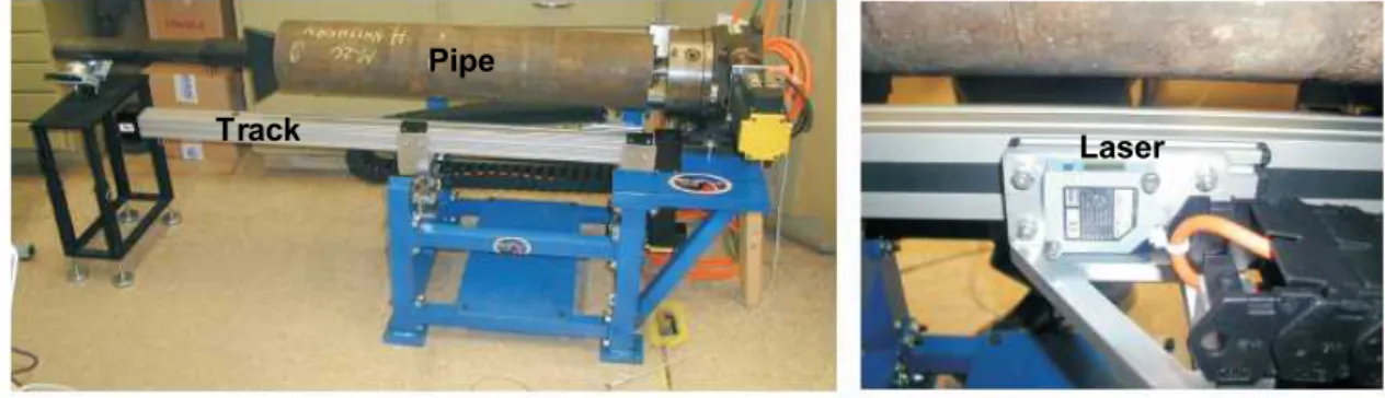
Individual pipe segments, typically 5.5 m or 6.1 m (18 or 20 ft) long, were tagged sequentially as they were removed from the trench, and subsequently cut into sections of about 1.1 m (3½ ft) long, to be scanned by a pipe laser scanner that was specially developed for this purpose (Figure 1). Prior to scanning, the exterior surfaces of the pipe sections were sandblasted to reveal
“corroded” or “graphitized” ductile iron. The contractor/sand blasters were instructed to use low nozzle velocities and avoid excessive blast times to prevent metal abrasion as well as to
immediately cut back on both if “blistering” or “slivering” occurred. This resulted normally in dull light gray pipe surfaces. The data from St. Louis pipes were only partially usable due to inadequate tagging and labeling, therefore these data were not used in the ring-based analysis.
Figure 1. Pipe scanner (left: pipe mounted ready for scanning; right: laser point range finder mounted on track).
Pipe
Figure 2. Schematic representation of pipe scanner data.
Pipe scanning involves the back and forth movement of a laser range finder mounted on a track that is placed parallel to the longitudinal pipe axis. When the laser range finder reaches either end of the pipe, the pipe rotates a specified amount, depending on the desired scan resolution and the pipe diameter. For every data point the scanner records the longitudinal distance x along the pipe, the rotation θ, and the distance ρ from the laser range finder to the pipe surface (Figure 2). The pipe scanning process terminates when θ reaches 360 degrees. The scanning resolution was set to provide data points spaced at 1.5 mm grid (i.e., 1.5 mm spacing along both longitudinal and circumferential directions).
Raw data obtained from the scanner can typically suffer from a number of problems. For
example, the scan data will show a pipe surface that looks warped or bent if the pipe section was not perfectly aligned in the pipe scanner. Also, under some conditions (oily pipe surfaces, asphaltic residue on the pipe, especially near repairs and service connections) the laser range finder sometimes had problems reading the pipe surface accurately, often indicating through-holes where there were none. Also, the scanning accuracy can diminish when a pit grows inside the pipe wall (with only a small opening at the surface). Using software specially developed for this purpose, a six-step process was used to record the data and remove these undesired effects: (a) read in raw data and apply a raw data filter; (b) rearrange the data into a grid; (c) establish the “correct” pipe surface; (d) apply 2-D grid-level filter; (e) apply 3-D grid-level filter; and (g) remove unusable data for statistical analysis. Details on the various filters applied to the data can
x
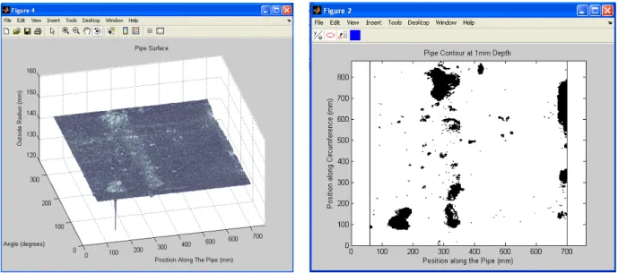
be found in Rajani et al. (2011). The results of this data cleansing process can be visualized as illustrated in Figure 3.
Figure 3: Data visualization: 3-D foldout (left) and pit contour (right).
Statistical analyses were conducted on geometrical properties of corrosion pits including pit-depth maxima, pit-area and pit-volume that were generated from the cleansed scanned data. Two different approaches were investigated as to the definition of the corrosion pit populations to which statistical analysis should be applied, namely individual pit populations and pipe ring populations. These are described in detail in the next two sections.
Definition and analysis of individual pit population
Corrosion pits are naturally small upon initiation and some will grow over time while others will become passivated (Aziz, 1956, used the term “stifled” and Melchers, 2005c referred to them as metastable (passivated) and stable pits). If two pits in close proximity continue to grow they will eventually combine (coalesce) to form one larger pit. This larger pit can continue to grow and may combine with yet more adjacent pits to become an even larger pit. This corrosion pit morphology presents a challenge as to what constitutes a single pit and its associated geometric properties. In this research the notion of threshold depth was used to define a single pit.
Figure 4 illustrates two adjacent corrosion pits that partially coalesced into one. If “Threshold 1” is taken as a reference then we have one corrosion pit with length X1 and maximum depth = (wall thickness - Y2). If “Threshold 2” is taken as a reference then we have two corrosion pits with lengths X2 and X3 and depths = (wall thickness - Y2) and = (wall thickness - Y3),
respectively. It is thus clear that a population of pits generated with threshold x is different from a population of pits generated with threshold y, and one population is not a subset of the other. For each of the four cities, three pit populations were generated, with three different threshold depth values as described in Table 2. Note that higher threshold depths result in a lower number of corrosion pits in the population. This is expected because for example, all pits with depth smaller than 2 mm are not considered when the threshold depth is 2 mm. However, note also that the number of through-holes can increase as the threshold depth increases. This can be explained with the help of Figure 4. Suppose that Y2 and Y3 were zero, i.e., there would be two through-holes in these locations. If the reference threshold depth is “Threshold 2” then there are two pits, each with depth exceeding wall thickness, i.e., two through-holes. However, if the reference threshold depth is “Threshold 1”, then there is only one pit with maximum pit depth exceeding wall thickness. In this case a through-hole is counted only once, even though there could be multiple perforations within the pit.
Figure 4. Corrosion pits and threshold depth
Y3 Y2
Table 2 Pit populations generated with various threshold depth values
Depth (mm) Area (mm2) Volume (mm3)
Threshold
depth # pits # through holes Min. Max. Min. Max. Min. Max.
Calgary 1 mm 10,346 24 1.0 8.44 2 33,208 2 81,996 2 mm 3,451 27 2.0 8.44 2 15,438 4 58,246 4 mm 1,059 42 4.0 8.44 2 6,455 9 39,812 Kansas City 1 mm 29,380 12 1.0 10.89 2 35,791 2 78,970 2 mm 2,732 12 2.0 10.89 2 14,868 4 47,613 4 mm 219 12 4.0 10.89 2 3,296 9 21,760 Louisville 1 mm 13,454 15 1.0 8.89 2 39,017 2 91,732 2 mm 2,074 17 2.0 8.89 2 21,830 4 65,014 4 mm 309 18 4.0 8.89 2 4,199 9 27,416 St. Louis 1 mm 17,904 11 1.0 10.51 2 66,107 2 161,202 2 mm 2,195 12 2.0 10.51 2 35,178 4 109,139 4 mm 207 12 4.0 10.51 2 4,754 9 34,358
Three different probability distributions as well as their right-truncated variants were examined as candidates to describe the populations of pit-depth maxima, pit-area and pit-volume. The right-truncated variants were explored because the properties of the pit populations are (or can be) right-truncated. For example, the value of pit depth is limited by the pipe wall-thickness, which in this case would serve as the upper bound of the truncated probability distribution. The distributions explored included Weibull (2-parameter),
] ) ( exp[ ) ( ) ( ] ) ( exp[ 1 ) ( 1 x x x f x x F (1)
where F(x) is the cumulative density function (cdf), f(x) is the probability density function (pdf),
] ) ( exp[ 1 1 ] ) ( exp[ 1 ) ( 0 ; ] ) ( exp[ ) ( ) ( 1 o o o x K x K x F x x x x x x K x f (2)
where xois the upper bound (truncation value) of the distribution. Gumbel (or double-exponential) distribution is,
)] exp( exp[ ) ( )] exp( exp[ ) ( 1 x f x x x x F (3)
where is the location parameter and is the scale parameter; and the right-truncated variant is,
)] exp( exp[ 1 )] exp( exp[ ) ( 0 ; )] exp( exp[ ) ( 1 o o o x K x K x F x x x x x x K x f (4)
And finally, the exponential distribution is,
) exp( ) ( ) exp( 1 ) (x x f x x F
(5)where 1/is the mean rate of occurrence, and its right-truncated variant is,
) exp( 1 ) exp( ) ( 0 ; ) exp( ) ( o o o x K x K x F x x x x x K x f (6)
Probability distribution parameters were discerned using the maximum likelihood method. Pearson’s chi-square test was used to ascertain “goodness of fit” between model and data (in all cases there were sufficient data to warrant chi-square test). Through holes were excluded in the
exploration of probability distributions for pit-depth maxima because they comprise an ever-increasing category of pits with constant depth, which would bias the distribution.
Figure 5 provides insight into the statistical properties of pit-depth maxima, where the pit populations are derived with to= 1 mm and 2 mm threshold depths as reference. Relative frequencies are shown at the top, followed by a right-truncated Weibull distribution fit that was found to best fit the pit-depth maxima data. Note that while the right-truncated Weibull
distribution has support in (or is defined on) the range x [0, xo], the pit-depth maxima data lie in the range [to, xo]. Consequently, the maximum likelihood method was applied to the variate x’
= (x - to) and the results were subsequently transformed back to actual pit-depth maxima. Quality of fit was assessed using the likelihood ratio (LR) test and the results are provided using the P-value, which can be loosely interpreted as “what is the probability of observing such quality of fit (between observed and modeled frequencies) without these frequencies actually belonging to the same probability distribution”. Therefore, a lower P-value reflects a better fit. It can be seen that the truncated Weibull distribution fits the pit-depth maxima data very well. As explained earlier, through-holes were excluded from the analysis of pit-depth maxima.
The bottom of Figure 5 illustrates the plotting position of the data, linearized using the assumed right-truncated Weibull probability distribution. Data that are perfectly distributed according to the assumed model will appear as a straight line on such a linearized plot. Note that in the plotting position the variate x’ = (x - to) cannot be transformed back to the true pit depth scale because of the logarithmic horizontal axis. Data with to= 1 mm appear to be fairly linear for the most part, except at the lower tail of the distribution. This deviation from straight line of the lower tail is all but eliminated for to= 2 mm, which suggests that the deviation could be
attributed to the various data filtering methods that were applied during data preparation which may have created some distortion in the very small values.
0.00 0.05 0.10 0.15 0.20 0.25 0.30 0.35 0.40 0.45 0 2 4 6 8 10 Re la ti ve fr eq ue nc y Pit depth
Chi square test = 0.04 (P-value = 0.000)
Truncated Weibull distribution
0.00 0.20 0.40 0.60 0.80 1.00 0 2 4 6 8 10 Re la tiv e fr eq ue nc y Pit depth Relative frequency 1 mm pit threshold 0.00 0.05 0.10 0.15 0.20 0.25 0 2 4 6 8 10 Re la ti ve fr eq ue nc y Pit depth 2 mm pit threshold 2 mm pit threshold
Chi square test = 0.021 (P-value = 0.000) 0.00 0.20 0.40 0.60 0.80 1.00 0 2 4 6 8 10 Re la tiv e fr eq ue nc y Pit depth 1 mm pit threshold
Chi square test = 0.04 (P-value = 0.000) 0% 20% 40% 60% 80% 100% 0 2 4 6 8 10 0.001 0.010 0.100 1.000 10.000
Log pit depth Theoretical distribution
Shape = 0.70 Scale = 0.59
Plotting position of
observed data 1 mm pit threshold
0% 20% 40% 60% 80% 100% 0 1 2 3 4 5 6 7 8 9 0.001 0.010 0.100 1.000 10.000
Log pit depth
Theoretical distribution Shape = 0.872 Scale = 1.064 2 mm pit threshold Linearized truncated Weibull plotting position (x’ = x - to)
Figure 5. Statistical properties of pit-depth maxima (Calgary) with 1 and 2 mm threshold depth Similar results (not shown here) were obtained for the pit data in Kansas City, Louisville and St. Louis. It appears that these results do not support Aziz’s (1956) observation regarding an
underlying distribution that is bimodal, where an exponential distribution describes the “stifled” pits, while the pits that continued to corrode are described by a bell-shaped distribution. This discrepancy might be explained by (a) the difference in material type (aluminum vs. ductile iron), (b) the difference in environment (emersion in water vs. pipe buried in soil), and (c) the difference in exposure time (a few months vs. many years). It could be postulated, that Aziz’s (1956) bell curve is said to shift to the right as the exposure time increases, and that since the Calgary pipe has been exposed in the ground for about 4 decades it is possible that this bell curve shifted far to the right, beyond the pipe wall thickness. However, this postulation is impossible to verify with the Calgary data set. Moreover, the through-hole state is an absorbing state, i.e., over time more and more pits will become through-holes but there is no evidence to suggest that the relative frequency of the very deep pits (that have not yet become through-holes) also increased. The same analysis was repeated for to= 4 mm and results were similar to those observed for
to= 2 mm, except that the P-values were somewhat higher (i.e., not as good a fit). Examination of data sets comprising pit-area and pit-volume revealed that these data sets were extremely skewed in all cities (between 97% and 99.5% of the data points were concentrated in the lower 2.5% of the range of values) therefore further statistical investigation was not pursued.
In summary, the right-truncated Weibull probability distribution was found to fit best the observed frequencies in all four data sets, i.e., Calgary, Kansas City, Louisville and St. Louis, and therefore was deemed to be the most likely underlying probability distribution of pit-depth maxima, regardless of the threshold depth value toused. In some cases, the non-truncated and truncated exponential distribution also fit the data fairly well, but never as well as the right-truncated Weibull distribution. This finding is in contrast to observations made by Aziz (1956), and as noted earlier also by Sheikh et al (1989), who assumed the truncated exponential
distribution and Sheikh et al. (1990), who assumed the normal distribution of the square root of pit depth at the early stage of corrosion and lognormal in the more advanced stages of corrosion.
Definition and analysis of ring population
Each of the exhumed pipes was virtually sliced into rings (or sections) of length x, where x = 25, 50, 100, 150, 300, 450 and 600 mm. Thus for example, an exhumed pipe of 10 m length would produce a population of 400 rings each 25 mm long, or a population of 200 rings each 50 mm long, and so on. In this way each exhumed pipe was tested seven different times with seven different ring populations. For each population, three pit properties were investigated, namely the distribution of pit-depth maxima in the rings, the distribution of the total corroded surface area (pit-area) in a ring and the distribution of metal volume loss due to corrosion (pit-volume) in a ring. Ring analysis was not performed on St. Louis data for reasons explained earlier.
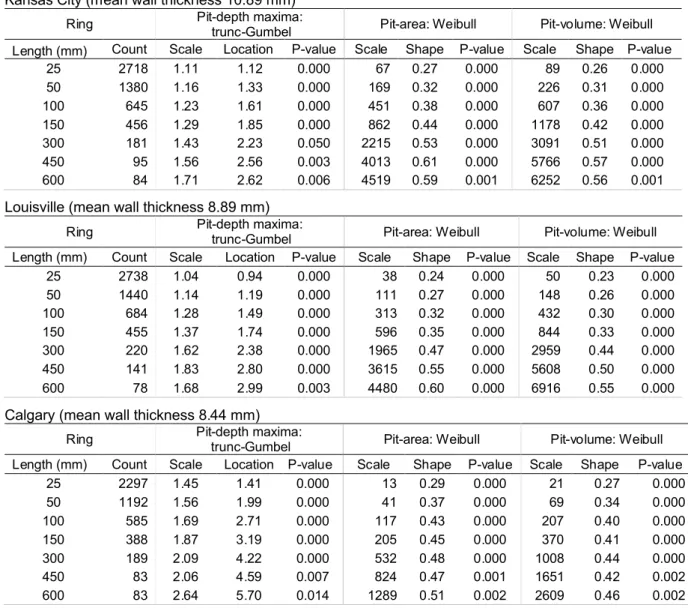
Each ring population was fitted with six different probability distributions (equations 1 through 6). For data sets comprising pit-depth maxima, the right-truncated Gumbel distribution was the most consistent in yielding low (often the lowest) P-values among all the cases tested. This bodes well with theoretical expectations because it is an extreme value distribution and the population at hand is indeed truncated. For the data sets comprising area, as well as those comprising pit-volume, among all the cases tested the Weibull distribution was the most consistent in yielding low (often the lowest) P-values. In most cases involving pit-area and pit-volume, the non-truncated distribution results did not differ much from their non-truncated variants. This is expected because none of the rings in any of the cities had its entire surface covered with corrosion pits (and certainly the entire volume could not have been depleted by corrosion). Statistical analyses results for each utility are provided in Table 3.
Table 3. Statistical analysis results of pit geometries in ring populations
Kansas City (mean wall thickness 10.89 mm)
Ring Pit-depth maxima:trunc-Gumbel Pit-area: Weibull Pit-volume: Weibull Length (mm) Count Scale Location P-value Scale Shape P-value Scale Shape P-value
25 2718 1.11 1.12 0.000 67 0.27 0.000 89 0.26 0.000 50 1380 1.16 1.33 0.000 169 0.32 0.000 226 0.31 0.000 100 645 1.23 1.61 0.000 451 0.38 0.000 607 0.36 0.000 150 456 1.29 1.85 0.000 862 0.44 0.000 1178 0.42 0.000 300 181 1.43 2.23 0.050 2215 0.53 0.000 3091 0.51 0.000 450 95 1.56 2.56 0.003 4013 0.61 0.000 5766 0.57 0.000 600 84 1.71 2.62 0.006 4519 0.59 0.001 6252 0.56 0.001
Louisville (mean wall thickness 8.89 mm)
Ring Pit-depth maxima:trunc-Gumbel Pit-area: Weibull Pit-volume: Weibull Length (mm) Count Scale Location P-value Scale Shape P-value Scale Shape P-value
25 2738 1.04 0.94 0.000 38 0.24 0.000 50 0.23 0.000 50 1440 1.14 1.19 0.000 111 0.27 0.000 148 0.26 0.000 100 684 1.28 1.49 0.000 313 0.32 0.000 432 0.30 0.000 150 455 1.37 1.74 0.000 596 0.35 0.000 844 0.33 0.000 300 220 1.62 2.38 0.000 1965 0.47 0.000 2959 0.44 0.000 450 141 1.83 2.80 0.000 3615 0.55 0.000 5608 0.50 0.000 600 78 1.68 2.99 0.003 4480 0.60 0.000 6916 0.55 0.000
Calgary (mean wall thickness 8.44 mm)
Ring Pit-depth maxima:trunc-Gumbel Pit-area: Weibull Pit-volume: Weibull Length (mm) Count Scale Location P-value Scale Shape P-value Scale Shape P-value
25 2297 1.45 1.41 0.000 13 0.29 0.000 21 0.27 0.000 50 1192 1.56 1.99 0.000 41 0.37 0.000 69 0.34 0.000 100 585 1.69 2.71 0.000 117 0.43 0.000 207 0.40 0.000 150 388 1.87 3.19 0.000 205 0.45 0.000 370 0.41 0.000 300 189 2.09 4.22 0.000 532 0.48 0.000 1008 0.44 0.000 450 83 2.06 4.59 0.007 824 0.47 0.001 1651 0.42 0.002 600 83 2.64 5.70 0.014 1289 0.51 0.002 2609 0.46 0.002
Impact of soil properties on the geometry of corrosion in ring populations.
Multi-covariate models. Two statistical models were proposed to assess the impact of soil
properties on corrosion in ring population. , These models are in fact the multi-covariate versions of the probability distributions that had been found (see previous section) to best fit the data. These include the right-truncated Gumbel distribution for pit-depth maxima and the Weibull distribution for pit-area and pit- volume. Equation (7) depicts a multi-covariate truncated Gumbel distribution, where the location parameter λ is a function of soil properties:
) exp( ) ( )] ) ( exp( exp[ 1 )] ) ( exp( exp[( ) ( 0 ; )] ) ( exp( ) ( exp[ ) ( 1 βz s s x K s x K x F x x x x s x s x K x f o o o (7)
where x is maximum pit depth in a ring, f(x) is the density function, F(x) is the cumulative probability, xois the upper bound of the truncated distribution, α is the scale parameter, λ(s) is the location parameter, which is a function of soil properties s, z is a row vector of soil properties (e.g., soil resistivity, redox potential, etc.) and β is a column vector of soil property coefficients to be discerned by the maximum likelihood method. Equation (8) depicts a multi-covariate Weibull distribution, where the scale parameter α is a function of soil properties
) exp( ) ( ] ) ) ( ( exp[ 1 ) ( ] ) ) ( ( exp[ ) ) ( ( ) ( ) ( 1 βz s s x x F s x s x s x f (8)
where, γ is the shape parameter, α(s) is the scale parameter, which is a function of soil properties s, z is a row vector of soil properties and β is a column vector of soil property coefficients to be discerned by the maximum likelihood method.
The essence of analyzing the impact of soil properties on corrosion pits was to determine whether, and by how much can soil property data, through multi-covariate probability
distributions, improve the ability to predict (or “explain”) observed variations in pit properties (pit-depth maxima, pit-area, pit-volume) beyond the single-variate probability distributions that were fitted to these properties as described in the previous section. The determination whether an additional covariate(s) actually improves the predictive ability of a model in a statistically
significant manner was done using the likelihood ratio (LR) test (e.g., Ansel and Phillips, 1994), )] ( ) ( [ 2 ) ( ) ( ln
2 MLL reducedmodel MLL fullmodel
model full ML model reduced ML LR (9)
degree of freedom (if it is reduced by two covariate then LR would be asymptotically chi-square distributed with two degrees of freedom and so on). In this research 5% was considered
significant for the P-value (≤ 0.05).
Soil properties data preparation. Table 4 provides a summary of the soil properties used in this research. The analysis of the impact of soil properties on the corrosion along the pipe requires a value corresponding to each ring. Simple linear interpolation is rarely used for geo-spatial properties (such as soil properties) because it is deemed too crude and lacking in precision. Instead, the inverse distance weighting (IDW) interpolation method was used, which is based on the assumption that the value of a property at an unsampled point is the weighted average of known values of this property within the neighborhood. These weights are inversely related to the distances between the unsampled point location and the sampled point locations. In this research weights were taken as the inverse of the square distance (full details are provided in Rajani et al., 2011).
In addition to soil properties data, metallic appurtenances and other metallic structures were documented along the exhumed pipes (e.g., couplings, service connections repair bands, valves, etc). The proximity to these metallic appurtenances (represented by the covariate
“Appurtenance” in Tables 5 and 6) was also investigated for its impact on observed corrosion pit properties.
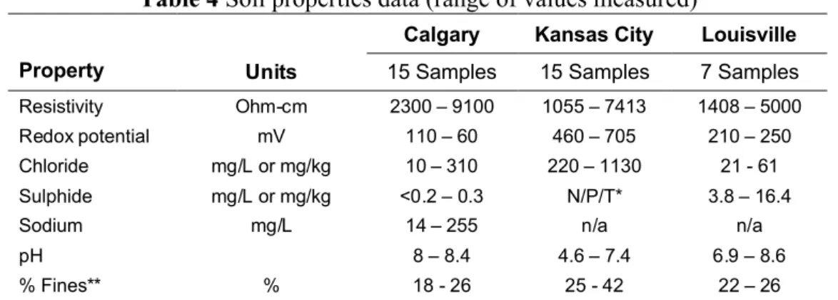
Table 4 Soil properties data (range of values measured)
Calgary Kansas City Louisville
Property Units 15 Samples 15 Samples 7 Samples
Resistivity Ohm-cm 2300 – 9100 1055 – 7413 1408 – 5000 Redox potential mV 110 – 60 460 – 705 210 – 250 Chloride mg/L or mg/kg 10 – 310 220 – 1130 21 - 61 Sulphide mg/L or mg/kg <0.2 – 0.3 N/P/T* 3.8 – 16.4
Sodium mg/L 14 – 255 n/a n/a
pH 8 – 8.4 4.6 – 7.4 6.9 – 8.6
% Fines** % 18 - 26 25 - 42 22 – 26
*Measured only negative (N)/positive (P)/trace (T). ** Defined as percentage of clay in the soil
A cautionary note is warranted with regards to analysis of soil properties impact on corrosion pits. In all exhumed samples, corrosion pits had been developing over an exposure period spanning several decades, while the soil properties were measured only at the time of
exhumation. Drawing quantitative conclusions about the impact of soil properties on corrosion, based solely on these soil samples, introduces an implicit assumption that these soil properties have remained more or less unchanged over the exposure period. This implicit assumption is impossible to verify in this field study and may not be true for all of these properties.
0 10 20 30 40 50 60 70 80 90 100 0 1 2 3 4 5 6 7 8 9 0 20 40 60 80 100 M ax p it de p th (m m ) Length (m) Re sis tiv ity 0 10 20 30 40 50 60 70 80 90 100 0 1 2 3 4 5 6 7 8 9 0 20 40 60 80 100 M ax p it de pt h (m m ) Length (m) Re sis tiv ity 0 10 20 30 40 50 60 70 80 90 100 0 1 2 3 4 5 6 7 8 9 0 20 40 60 80 100 M ax p it de p th (m m ) Length (m) Re sis tiv ity 0 10 20 30 40 50 60 70 80 90 100 0 1 2 3 4 5 6 7 8 9 0 20 40 60 80 100 M ax p it d ep th (m m ) Length (m) Re sis tiv ity 600 mm rings Coeff. =-0.006 P-value = 0.079 300 mm rings Coeff. = -0.006 P-value = 0.009 100 mm rings Coeff. = -0.005 P-value = 0.001 50 mm rings Coeff. = -0.005 P-value = 0.000
Analysis results. As an example, Figure 6 illustrates the relationships between maximum pit depth and soil resistivity for various ring length populations in Calgary. The small dots represent maximum pit depth in each ring (left axis) and the curve represents soil resistivity along the pipe (the markers on the curve are actual measured values in the soil samples and the curve represents the interpolated values). It can be seen that although such a relationship is not visually apparent, the relatively low P-values indicate that it exists to some extent. Furthermore, the coefficients obtained for the resistivity covariates were all negative, which confirmed the expected type of impact, i.e., low resistivity results in high corrosion and vice versa.
In the analysis to assess the impact of soil properties on corrosion, each of these properties was considered in two ways, absolute values and rate of change (derivative) values, where rate of change value is calculated between two adjacent soil sample locations as the difference in the soil property values divided by the distance between these two points. In addition, the distance of a ring from an appurtenance or a service connection or a repair band, etc. was considered as well. This results in a total of 13 covariates (six based on absolute values of soil properties, six based on their derivatives and one based on the distance from appurtenance). An exhaustive
examination requires the LR computation of all combinations of covariates (i.e., each covariate on its own (single) – 13 cases; all possible combinations of two covariates (pair) - = 78 cases; all possible combinations of three covariates (triplet) - = 286 cases and so forth) totaling many thousands of cases, applied to three corrosion pit properties (maximum depth, area and volume), each with 4 possible ring lengths (50, 100, 300 and 600 mm). However, careful
observation can often reduce the number of combinations requiring examination to a manageable number of a few hundred (for each of the exhumed pipes from the respective cities).
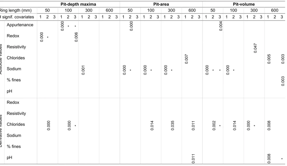
Table 5 provides the results for the multi-covariate analysis of the Calgary data. A few comments, explanation and observations are warranted:
Table 5 shows P-values, rounded off to 3 decimal places. Only those that are significant at the 5% level (i.e., P-value ≤ 0.05) are shown.
Table 5. Calgary Data: P-values of various covariates in various ring lengths (only P-values smaller or equal to 0.05 are shown)
Pit-depth maxima Pit-area Pit-volume
Ring length (mm) 50 100 300 600 50 100 300 600 50 100 300 600 # signif. covariates 1 2 3 1 2 3 1 2 3 1 2 3 1 2 3 1 2 3 1 2 3 1 2 3 1 2 3 1 2 3 1 2 3 1 2 3 Absolu te values Appurtenance 0.000 * * 0.000 0.004 Redox 0.000 * 0.006 Resistivity 0.047 Chlorides 0.007 0.005 0.003 Sodium 0.001 0.000 * 0.000 * 0.000 * 0.000 * * 0.000 * % fines 0.003 pH Derivative values Redox Resistivity Chlorides 0.000 0.000 * 0.014 0.035 0.011 0.002 * 0.014 0.000 * 0.008 Sodium % fines pH 0.011 0.008 *
Three columns, 1, 2 and 3 are provided for each ring length. Column 1 shows the P-value for the single most statistically significant covariate. Column 2 shows the P-value for the most statistically significant pair of covariates and column 3 shows the P-value for the most statistically significant triplet of covariates. The marginal contributions to LR of more than three covariates (pH, redox and resistivity) were insignificant for all cases examined for Calgary, however, in some cases as many as a quintuple of covariates (Kansas City) was found significant, and in another case as few as a single covariate (Louisville).
It interesting to note that soil resistivity, which is often considered as the single most significant factor in pipe corrosion, was not found to be a significant covariate to explain corrosion on ductile iron pipe in Calgary.
If a generic covariate A is the single most statistically significant covariate and generic covariates A and B are the most statistically significant pair of covariates, then A’s P-value is provided in column 1, and P-P-value in column 2 for covariate A is represented by an asterisk (*). Covariate B will have a P-value in column 2, indicating its marginal contribution to the LR of the covariate pair A and B is beyond the contribution of covariate A alone. The same logic is extended to the case of three covariates or more. If covariate A is the single most statistically significant covariate and covariates B and C
are the most statistically significant pair of covariates, then A’s P-value is provided in column 1, and the value of covariates B and C is provided in column 2. This latter P-value indicates the contribution to the LR of the covariate pair of B and C beyond the baseline, i.e., beyond the maximum likelihood value of the model with no covariates (where the LR is computed with two degrees of freedom). The same logic is extended to the case with three covariates or more.
In Calgary, soil sodium concentration appears to be consistently significant. It emerged as the single most significant covariate in 6 out of 11 cases shown in Table 5. Out of these 6 cases, it also emerged 5 times as one of the two covariates in the most significant pair, and 1 time as one of the three covariates in the most significant triplet. Unfortunately, Calgary was the only utility that measured sodium concentration in soil samples,
therefore this relatively high significance of sodium concentration could not be compared to analyses of other cities.
The derivative of chloride concentration also showed consistent significance. In 1 out of 11 cases, it was the single most significant covariate. In 6 out of 11 cases, it was one of the two covariates in the most significant pair. In 3 out of 11 cases, it was one of the three covariates in the most significant triplet.
Proximity to appurtenance did not emerge as consistently significant covariate. In 1 out of 11 cases, it was the single most significant covariate. In 2 out of 11 cases, proximity to appurtenance was one of the two covariates in the most significant pair. In 2 of 11 cases, proximity to appurtenance was one of the three covariates in the most significant triplet. Pit-depth maxima results for 600 mm rings could not be obtained in Calgary data due to
some numerical problems that could not be resolved.
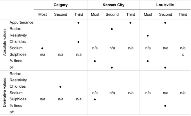
Similar analyses were carried out for the Kansas City and Louisville data. Tables with full results are not provided here due to space limitations although full details can be found in Rajani et al., 2011). Instead, Table 6 shows which covariates emerged as the most/second/third consistently significant in the respective data sets, including all ring lengths and including pit depth
maximum, pit area and pit volume (“n/a” means that the covariate was not measured in the respective cities).
Table 6. Most consistently significant covariates
Calgary Kansas City Louisville
Most Second Third Most Second Third Most Second Third
Absolute values
Appurtenance
Redox
Resistivity
Chlorides
Sodium n/a n/a n/a n/a n/a n/a
Sulphides n/a n/a n/a x
% fines pH Derivative values Redox Resistivity Chlorides
Sodium n/a n/a n/a n/a n/a n/a
Sulphides n/a n/a n/a
% fines
pH
It is quite clear that the three data sets (Calgary, Kansas City, Louisville) reflect high variability, in that no single soil property or combination of properties appeared to emerge as consistently significant in pipes from all three utilities.
The fact that some covariates were found to be statistically significant means that these
covariates appear to have some influence on the observed geometrical properties of the corrosion pits in the rings. However, it is not clear to what extent these covariates might improve the actual prediction of corrosion pit properties. A better insight into this improvement can be obtained by comparing the observed pit geometry to the pit properties calculated using the discerned
coefficients. This comparison of the predicted (calculated) means with observations can be assessed through the “goodness of fit” measure of the unadjusted coefficient of determination (R2):
2 2 2 ) ( ) ( 1 observed i i i Y Y Y Y R observed observed calculated (10)where Yiare pit geometry properties (maximum depth, area or volume). The coefficient of determination, R2, measures how much calculated (or modeled) values are able to estimate observed values better than a simple mean estimate. R2= 0 means that the model is no better than a simple mean, while R2= 1 means that the model has perfect prediction ability (a negative value is possible too, indicating worse that the mean). Theoretically, an adjusted coefficient of
determination should be used in multi-covariate models since it accounts for the goodness of fit as well as the loss of degrees of freedom (to identify a parsimonious model). In our case, an unadjusted coefficient of determination was used since we are only interested in the goodness of fit (significant covariates were already identified based on LR test).
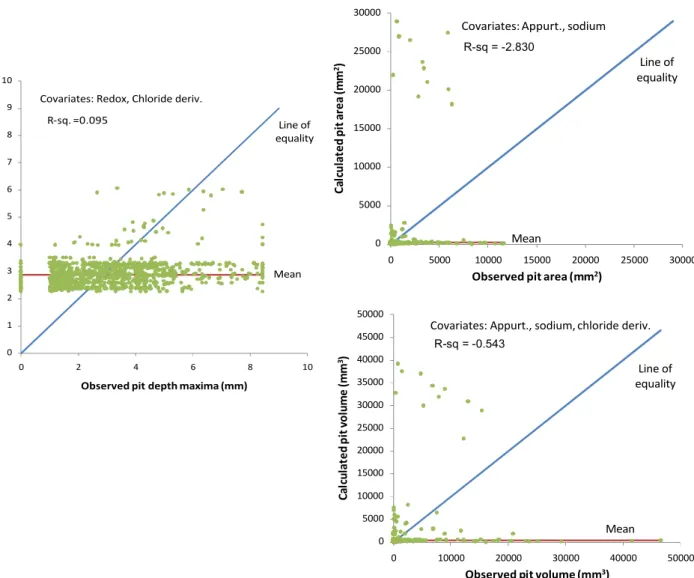
Figure 7 illustrates the R2obtained for the pit geometries in 50 mm rings using covariates that were found to be statistically significant in Calgary. It can be seen that R2of the pit-depth maxima improved somewhat (to 0.095, indicating that the soil-related covariates helped in predicting mean pit-depth maxima. However, pit-area and pit-volume predictions degraded with the introduction of soil-related covariates, despite the fact that these covariates were found to be statistically significant by the LR test. Similar results were obtained in the Kansas City and Louisville data sets, where R2of the pit-depth maxima improved somewhat (to 0.161 and 0.058 in Kansas City and Louisville, respectively) but R2degraded for pit-area and pit-volume
Figure 7. Calgary (50 mm rings) predicted means vs. observed pit properties
It should be noted that likelihood ratio tests do not measure exactly what R2endeavors to measure, therefore it is possible to see these types of apparent “contradictions”. These contradictions become less likely as the significance of the covariate increases.
Summary and conclusions
Pit population. The pit population analysis examined the statistical properties of corrosion pits.
Line of equality 0 1 2 3 4 5 6 7 8 9 10 0 2 4 6 8 10 Ca lc ul at ed m ea n pi t d ep th m ax im um (m m )
Observed pit depth maxima (mm)
R-sq. =0.095
Mean Covariates: Redox, Chloride deriv.
Line of equality 0 5000 10000 15000 20000 25000 30000 0 5000 10000 15000 20000 25000 30000 Ca lc ul at ed p it ar ea (m m 2)
Observed pit area (mm2) R-sq. =0.000
Mean
Covariates: Appurt., sodium R-sq = -2.830 Line of equality 0 5000 10000 15000 20000 25000 30000 35000 40000 45000 50000 0 10000 20000 30000 40000 50000 Ca lc ul at ed p it vo lu m e (m m 3)
Observed pit volume (mm3) R-sq. =0.000
Mean Covariates: Appurt., sodium, chloride deriv.
Louisville and St. Louis), using three different threshold depth reference values (1, 2 and 4 mm). The right-truncated Gumbel probability distribution was found to fit the observed distribution of depth maxima quite well in all 12 populations. The observed distributions of area and pit-volume were too unbalanced to warrant the fitting of any theoretical probability distribution. The investigation of pit populations was conducted to expand on existing knowledge and to compare findings with those of other researchers rather than for any practical purpose. It is much more practical to create sampling schemes and inference methods based on ring population rather than pit population. Practical sampling scheme would typically involve examination of a number of small pipe samples that represents the entire pipe. As the area of a single pit can vary significantly, sample sizes would have to be quite large to contain entire large pits. Furthermore, when a pipe is virtually divided into rings, the location of each ring can be easily related to the location of a soil sample. Moreover, ring-based analysis lends itself better to develop inference techniques that are based on return period computations (discussed in the companion paper Kleiner and Rajani 2011a) because a ring is always geometrically well defined.
Ring population without soil properties. Seven different ring populations were examined for each of three data sets (Calgary, Kansas City, Louisville). These seven populations included rings of lengths 25, 50, 100, 150, 300, 450 and 600 mm. The right-truncated Gumbel probability distribution was found to provide the best fit and in the most consistent manner to the observed frequency distribution of pit-depth maxima. The Weibull distribution fitted best and most consistently the observed frequency distributions of pit-area and pit-volume.
Ring population with soil properties impact. Multi-covariate probability distributions were assumed for ring populations, where covariates comprised various soil properties associated with ring location as well as ring distance from known appurtenances. For pit-depth maxima a multi-covariate right-truncated Gumbel distribution was assumed, where the location parameter is a function of soil properties. A multi-covariate Weibull distribution was assumed for pit-area and pit-volume, where the location parameter is a function of soil properties. Soil properties were interpolated between samples since they were sampled at discrete intervals. The multi-covariate probability distributions were examined on four populations drawn from each data set, including rings of lengths 50, 100, 300, and 600 mm.
No single soil property or combination of properties appeared to emerge as statistically significant in all three data sets (Calgary, Kansas City, Louisville). The impact of statistically significant soil properties towards the improvement in the predictability of expected mean corrosion pit properties in the rings was examined with the help of the coefficient of determination (R2). The introduction of soil properties improved the prediction of pit-depth maxima in virtually all cases, albeit not by much. However, soil properties most often degraded the pit-area and pit-volume predictions (compared to a simple mean value).
It can be concluded that the data on corrosion pits and soil properties from three different cities did not provide any compelling evidence to suggest that the knowledge of soil properties along the pipe improves the ability to predict corrosion pit properties in any significant or consistent manner. It is possible that better consistency among measured soil properties (sodium only in Calgary, sulphides not in Calgary, sulphides measured as yes/no/trace in Kansas City versus actual concentration in Louisville) would have increased the confidence in the results but are not likely to have changed them in any significant way. This apparent lack of impact of soil
properties on corrosion pit geometry seems to contradict a large body of work in the literature. Two plausible explanations for this contradiction are: first, as stated earlier, soil properties data in this research are but a snapshot picture, whereas the pipes have been buried for decades. It is possible that soil properties changed over time and therefore the observed corrosion pits do not exactly reflect exposure to current soil properties; second, our data sets presented relatively short pipes (~90 m or 300’) long. In general, soil properties do not vary significantly over such a short distance. In our data sets, with few exceptions (e.g., resistivity in Calgary – from 2,300 to 9,100 ohm-cm, pH in Kansas City – from 4.6 to 7.4), soil properties were relatively uniform. The companion paper Kleiner and Rajani (2011a) describes the development of sampling and statistical inference of the pipe condition that is based on the analysis presented here. Acknowledgement
This research project was co-sponsored by the Water Research Foundation (WaterRF), the National Research Council of Canada (NRC) and water utilities from the United States, Canada and Australia.
References
Ansell, J.I., and M.J. Phillips, (1994). “Practical methods for reliability data analysis”. Oxford University Press, Oxford, UK.
ANSI/AWWA C105/A21.5-99. (1999). “American National Standard for polyethylene encasement for ductile iron pipe systems”. American Water Works Association, Denver, CO. Aziz, P.M. (1956). “Application of the statisticall theory of extreme values to the analysis of maximum pit depth data for aluminum”. Corrosion 12, pp. 35-46.
Caleyo, F., Velázquez, J.C., Valor, A. and Hallen, J.M. (2009). “Probability distribution of pitting corrosion depth and rate in underground pipelines: A Monte Carlo study”. Corrosion Science, 51, pp. 1925–1934.
Hay, L. S. (1984). “The influence of soil properties on the performance of underground pipelines”. M.Sc.(Agriculture) thesis, Dept. Soil Science, University of Sydney, Sydney, Australia.
Katano, Y., Miyata, K., Shimizu, H. and Isogai, T. (1995). “Examination of statistical models for pitting on underground pipes and data analysis”. Proceedings of the International Symposium on plant aging and life prediction of corrodible structures, May 15-18, Sapporo, Japan..
Katano, Y., Miyata, K., Shimizu, H. and Isogai, T. (2003). “Predictive model for pit growth on underground pipes”. Corrosion, 59(2), pp. 155-161.
Kleiner, Y., and Rajani, B. (2011) “Long-term performance of ductile iron pipe”, Research report to be published by the Water Research Foundation, Denver, CO.
Kleiner, Y. and Rajani, B. (2011a) “Performance of ductile iron pipe: sampling scheme and inferencing pipe condition”. Submitted for publication in Journal of Infrastructure Systems, ASCE. New York, NY.
Laycock, P. J., R.A. Cottis, and P. A. Scarf (1990). “Extrapolation of extreme pit depths in space and time”. Journal of the Electrochemical Society, 137(1), pp. 64-69.
Melchers, R.E. (2003). “Modeling of marine immersion corrosion for mild and low alloy steels-Part 1: phenomenological model”. Corrosion (NACE), 59(4), pp. 319–334.
Melchers, R.E. (2004a). “Pitting corrosion of mild steel in marine immersion environment – Part 1: maximum pit depth”, Corrosion (NACE), 60(9), pp. 824-836.
Melchers, R.E. (2004b). “Pitting corrosion of mild steel in marine immersion environment - Part 2: variability of maximum pit depth”. Corrosion (NACE), 60(10), pp. 937–944.
Melchers, R.E. (2005a). “Statistical characterization of pitting corrosion – 1: Data analysis”. Corrosion (NACE), 61(7), pp. 655-664.
Melchers, RE (2005b) “Statistical characterization of pitting corrosion – 2: Probabilistic modelling for maximum pit depth”. Corrosion (NACE), 61(8), pp. 766-777.
Melchers, RE (2005c). “Representation of uncertainty in maximum depth of marine corrosion pits”. Structural Safety, 27, pp. 322-334.
Najjaran, H., Sadiq, R., and Rajani, B. (2006). "Fuzzy Expert System to Assess Corrosivity of Cast/Ductile Iron Pipes fromBackfill Properties". Computer Aided Civil and Infrastructure Engineering, 21(1), pp. 67-77.
Rajani, B., Kleiner, Y., and Krys, D. (2011) “Long-term performance of ductile iron pipe”, Research report to be published by the Water Research Foundation, Denver, CO.
Restrepo, A., Delgado, J. and Echeverría, F. (2009). “Evaluation of current condition and lifespan of drinking water pipelines”. Journal of Failure Analysis and Prevention. 9,pp. 541– 548.
Rossum, J. R. (1969). “Prediction of pitting rates in ferrous metals from soil parameters”. Journal American Water Works Association, AWWA, 61, pp. 305-310.
Sadiq, R., Rajani, B. and Kleiner, Y. (2004). "Fuzzy-Based Method to Evaluate Soil Corrosivity for Prediction of WaterMain Deterioration". Journal of Infrastructure Systems, 10(4), pp. 149-156.
Scarf, P. A, R.A. Cottis, and P. J. Laycock. (1992). “Extrapolation of extreme pit depths in space and time using the r deepest pit depths”. Journal of the Electrochemical Society, 139(9), pp. 2621-2627.
Sheikh, A.K., Boah, J.K. and Jounas, M. (1989). “Truncated extreme value model fro pipeline reliability”. Reliability Engineering and System safety, 25(1), pp. 1-14.
Sheikh, A.K., Boah, J.K. and Hansen, D.A. (1990). “Statistical modelling of pitting corrosion and pipeline reliability”. Corrosion-NACE, 46(3), pp. 190–197.
Spickelmire, B. (2002). "Corrosion consideration for ductile iron pipe". (NACE) Materials Performance, 41(7), 16-23.