OPTICS OF INSTANTANEOUS WAVES

HAL Id: hal-00004162

https://hal.archives-ouvertes.fr/hal-00004162

Submitted on 4 Feb 2005

HAL is a multi-disciplinary open access archive for the deposit and dissemination of sci-entific research documents, whether they are pub-lished or not. The documents may come from teaching and research institutions in France or abroad, or from public or private research centers.

L’archive ouverte pluridisciplinaire HAL, est destinée au dépôt et à la diffusion de documents scientifiques de niveau recherche, publiés ou non, émanant des établissements d’enseignement et de recherche français ou étrangers, des laboratoires publics ou privés.

OPTICS OF INSTANTANEOUS WAVES

Alexandr Shvartsburg, Guillaume Petite

To cite this version:

Alexandr Shvartsburg, Guillaume Petite. OPTICS OF INSTANTANEOUS WAVES. E. Wolf. Progress in Optics, vol. 44, Elsevier, pp.143-214, 2002. �hal-00004162�

OPTICS OF INSTANTANEOUS WAVES

By

Alexander B. SHVARTSBURG

Central Design Bureau for Unique Instrumentation of the RAS

Butlerov Str. 15, Moscow, Russia

and

Guillaume PETITE

Laboratoire des Solides Irradiés, CEA/DSM/DRECAM, CNRS (UMR 7642) and Ecole Polytechnique, 91128, Palaiseau, France

OUTLINE

INTRODUCTION

I. SHORT E.M. PULSES : HOW THEY ARE MODELED, PRODUCED, MEASURED.

I.1) Non sinusoidal waveforms of electromagnetic waves. I.2) Production of ultrashort EM pulses

I.3) Measurement of ultrashort EM pulses

II. SPATIOTEMPORAL RESHAPING OF ULTRASHORT PULSES IN STATIONARY

MEDIA

II.1) Dynamics of ultrashort waveforms in dispersionless optical systems II.2) Evolution of transients in dispersive media

II.3) Broadband reflectivity in transient optics

II.4) Diffraction induced transformations of ultrashort pulses in free space and dispersive media

III. OPTICS OF NON STATIONARY MEDIA

III.1) Non-stationarity induced dispersion in dielectrics

III.2) Dynamical regime in the reflectivity of non-stationary dielectrics III.3) Spectral distortions of waves reflected from a non-stationary dielectric CONCLUSION

ABSTRACT

This review is devoted to the transient optical phenomena, displayed both in the spatiotemporal dynamics of ultrashort single - cycle wave pulses in free space and dispersive dielectrics as well as to interaction of light with non-stationary media. The interplay of diffractive and dispersive phenomena, including the coupled processes of amplitude and phase reshaping, spectral

variations, polarity reversal for different types of light pulses, is examined in frequency and time domains. Reflection - refraction effects on the interfaces of media with time-dependent dielectric susceptibility are considered by means of exact analytical solutions of Maxwell equations for these media. The non - stationarity - induced dispersion is shown to provide a dynamical regime of reflectivity of non-stationary media, depending upon both instantaneous dielectric

susceptibility and its temporal derivative; the relevant generalization of Fresnel formulae is presented

INTRODUCTION :

This paper is devoted to the physical fundamentals and mathematical basis of the optics of waveforms whose parameters vary in the course of propagation. The dynamics of instantaneous optical fields, travelling in free space and continuous media, opens many new opportunities for controlled spatio-temporal reshaping of these fields. The ongoing interest towards such problems in fueled by several research goals:

- to optimize the processes of light pulses transfer through optical systems; this is particularly important in view of the applications to optical communication : the use of ultrashort pulses at high repetition rate is one of the approaches to the increase of the transfer rate.

- to develop methods of fast non-destructive testing of materials and targets, atmospheric sensing, using ultrashort broadband electromagnetic (EM) pulses;

- to reach a comprehensive understanding of such ultrafast processes as amplitude or phase modulation of EM waves interacting with non stationary media.

Moreover, an important task is to elaborate an analytical approach to these topics, which were considered until recently as an exclusive field of computer simulations.

The investigation of coupled processes of spatial and temporal deformations of localized waveforms is preceded here by a brief description of waveforms widely used in modeling of such processes. Both frequency and time-domain models are presented below in Section I-1. We then briefly recall how such waveforms are produced (I-2), and measured experimentally (I-3).

Two opposite statements of the problems of instantaneous optics will then be treated. Section II is focused on the spatio-temporal dynamics of localized EM pulses interacting with stationary dielectric media. On the contrary, the reshaping of harmonic CW trains interacting with non-stationary media is discussed in Section III. In this latter case, a special attention will be given to some exactly solvable models, providing a better physical insight into these problems.

I. ULTRASHORT EM PULSES : HOW THEY ARE MODELED, PRODUCED, MEASURED.

It is first necessary to agree upon what will be defined as an ultrashort electromagnetic pulse. Here we will retain the following definition : a pulse whose duration is of the order of a few, at most a few tens of periods of the EM field. It is of course almost equivalent to consider pulses whose spectral width is a substantial fraction of their frequency, except that one rather adresses in this case the coherence length of the pulse than its duration, so that this definition would be strictly valid for radiation presenting complete temporal coherence only, a criterion which is not even satisfied by all lasers. In this section, we will first recall some of the mathematical models which have been used to represent such pulses (§ I.1), and we will then briefly recall how such pulses are produced (§ I.2) and measured (§ I.3).

I.1) Non-Sinusoidal Waveforms of Electromagnetic Waves.

Let us begin this analysis from the traditional spectral approach. To optimize a waveform

( )

t E F

( )

t

E = ₀ with respect to a bandwidth-limited communication system or to the width of an absorption line, it is traditional to work with its Fourier transform (FT). Some properties of waveforms F(t), having an essential influence on their spectral bandwidths, such as their duration and rise time, are considered below.

I.1.1. Square-shaped truncated train of monochromatic waves, are represented by the function :

( )

( )

0 0 0 cos ; 0 ; t t t F t t t ω  _≤  =   > (1.1)

The spectral density of EM energy Ε

( )

∆ in a pulse F (1.1), localized in some finite spectral range (ω±∆ 2), writes

( )

( )

( )

0 0 2 2 2 0 2 1 ; 2 E W W F d ω ω ω ω π ∆ + ∆ − Ε ∆ = ∆ ∆ =

∫

(1.3)

The spectral density Ε calculated for an infinite spectral range, ∆→∞, is given by the function W(∞). The spectral bandwidth of a pulse is defined as the range of frequencies ω0±∆, containing some given fraction δ (e.g., δ = 90% or 99%) of the pulse energy

( )

∆ = ×W

( )

∞

W δ (1.4)

Substituting the Fourier amplitude F_ω (1.2) into (1.3) and introducing a variable x=t0∆ we

obtain the function W

( )

∆

( )

( )

      − = ∆ x x x Si t W 2 0 ₂ sin 2π (1.5)

where Si(x) is the integral sine function

∫

=x dy y y x Si 0 sin ) ( (1.6)

Using the value Si(∞)= π/2 , one can present eq. (1.4), governing the value of spectral-time product Kc=t0∆c , in a form

( )

πδ 2 sin 2 2 = − c c c K K K Si (1.7)

Considering the central part of the distribution F_ω (1.2), located between the zeros of F_ω (Kc=±π), one can see that 90% of the pulse energy is contained in the spectral range ω0±π/t0.

Any further significant growth of this fraction δ requires a substantial increase of spectral range : for δ = 0.99, the spectral range Κc is increasing by more than a factor 10.

It is worthwhile to compare the broadband square-shaped pulses, characterized by a short rise time, tending formally towards zero, with other waveforms possessing the same

I.1.2. To illustrate the influence of increasing rise- and falltime, let us consider the Gaussian-shaped waveform

( )

      − = ₂ 0 2 2 exp t t t F (1.8)

the FT of a Gaussian waveform is known to be also Gaussian

( )

_      − = 2 exp 2 2 0 0 t t F_ω π ω (1.9)

It is often convenient to characterize the pulse by its full width at half-maximum (FWHM). The Gaussian waveform (1.8) and its FT (1.9) are defined by the FWHM values tc and ωc

55 . 5 ; 35 . 2 ; 35 . 2 0 0 = = = _{c c c} c t t t t ω ω (1.10)

Using the first of relations (1.10), one can present the Gaussian profile (1.8) in a form, expressed via the FWHM

( )

_             − = 2 67 . 1 exp c t t t F (1.11)

Calculating the function W(∆) (1.3), related to the FT (1.9), we obtain the equation, governing the bandwidth ∆c

(

t ∆c

)

=δ

erf ₀ (1.12)

Here erf is the error function. Taking, e.g., δ=0.9, one has Kc=t0∆c=1.17, and thus the

bandwidth ∆c of the Gaussian pulse (1.8) is almost three times smaller than that of the

square-shaped pulse (Kc=π for δ=0.9). This example shows that an increase of rise time, the pulse

duration being fixed, induces a strong spectral narrowing.

Some pulses with extremely steep leading edges have been proposed as prospective carriers for directed energy transmission in free space. Such a pulse, entitled by Wu [1985] “electromagnetic missile”, yields a diffracted wave decaying slower than z-2 in intensity.

see that the boundaries of the first Fresnel zone zF=ω a2c-1 for high frequencies ω become

extremely distant. Wu [1985] showed that when the pulse spectrum is damping slowly in the high-frequency limit ω→∞, even though the energy collected on a detector of finite dimensions is still tending to zero when z→∞, it can be made to do so in an arbitrarily slow manner. An example of such pulses is expressed as a function of time via the modified Bessel function K of _ν

ν-th order:

( )

            = 0 0 t t K t t t F _ν ν (1.13)

Taking the cosine FT from (1.13), we obtain

(

)

2 1 2 0 2 0 0 1 1 2 1 2 + − +       ₊ Γ = ν ν ω ω ν π t t F (1.14) Presenting ν in a form ; 0 2 1 > + − = γ γ

ν , one finds as asymptotic spectral behavior of

γ ω

ω →∞≈ω−2

F ; thus, following Wu [1985], an appropriate choice of parameter γ yields an arbitrarily slow decrease of the high-frequency limit of (1.14), providing a weakened angular divergence of the pulse at distances z ≥ωa2c−1.

I.1.3. Until now we have discussed ways to broaden or to narrow the spectral bandwidths for waveforms of a given duration 2t0. Steepening of the pulse fronts was shown to cause an increase

of the spectral bandwidth; their softening can give rise to a narrowing of the spectrum. However, it should be mentioned that there is an implicit simplification in all the above developments, which is that we have not allowed statistical fluctuations between the different spectral

components of the EM field we studied. Any classical source will present such fluctuations, as well as most of the lasers. All the above developments thus deal with temporally coherent sources such as single longitudinal mode or mode-locked lasers. One often refers to such pulses as “Fourier Transform limited pulse” (in the sense that the bandwith of a partially coherent pulse

will be larger than strictly required by the FT). It should be mentioned that there is a stricter definition of a FT-limited pulse, which is the one having the narrowest pulse width possible for a given spectral amplitude distribution. The term “amplitude” may be misleading here since the spectral amplitudes are in reality complex, and the actual temporal shape of the pulse will depend on the shape of the “spectral phase” φ(ω) . Fig. 1 illustrates this point by comparing two pulses having the same power spectrum ( f

( )

ω 2), but different spectral phase behaviors. It shows that the pulse with the minimum width (and in this sense, strictly speaking FT-limited) is the one presenting a linear spectral phase frequency dependence.

The physical and computational problems, resulting from the efforts to adjust the Fourier “ω-k“ language to the dynamics of ultrashort waveforms in dispersive media, stimulated the development of time-domain models, i.e. directly using the temporal dependence of electric and magnetic strength of EM field, for such waveforms.

I.1.4. Models of pulses assuming equality of rise and fall times have been considered so far. However, there are many real optical pulses that do not have such symmetry. An example of strongly asymmetrical waveform, described by a Gaussian rising edge, followed by an exponentially falling tail

( )

2 1.67 exp ; 0 0 exp ; 0 0 0 t E t tC E t t E t t   _{ }    _{ }  − ≤   _{ }   _   _  =     _{ } − ≥  _{ }     (1.15)

was discussed by Qian and Yamashita (1992). This so-called single-cycle exponential waveform has a discontinuity of derivative at the maximum t = 0. A double- exponential waveform,

( )

            − −       − = 2 1 0 exp exp t t t t E t E (1.16)

was used by Ma and Ciric [1992] for the analysis of transient scattering on small targets; in the case (t1>>t2), profile (1.16) resembles a single-sided waveform, but differs from (1.15) by a

smooth maximum.

Flexible models, describing continuous waveforms with an arbitrary amount of different extrema and unequal distances between zero-crossing points, were used in time-domain optics by Shvartsburg [1999]. These waveforms, characterized by well-expressed leading fronts with finite slope, an arbitrary number of unharmonic oscillations and exponentially damping tails, are defined by the series of Laguerre functions Ln in the time interval 0≤ t < ∞

( )

∑

∞ =      = 0 0 n n n t t L a t E (1.17)

The Laguerre functions (Fig. 2)

( )

[

x

( )

x

]

dx d n x x L _n n n n −      ₋ = exp ! 2 exp (1.18)

are known to be orthonormal in the interval 0 ≤ x ≤∞, that is to say :

nm m n x L x dx L =δ

∫

∞ ) ( ) ( 0 (1.19)

These waveforms, localized in time, are suitable for description of plane wave pulses. However, to consider the dynamics of both spatially and temporally localized fields, other families of waveforms are needed.

I.1.5. The spatiotemporal structure of few-cycle three-dimensional pulsed wave beams can be described by means of so-called Poisson-spectrum pulses

( )

( )

( )

m it t it t f t ef t F _       + = ℜ = 0 0 ' ; (1.20)

Here ℜef indicates the real part of the function f(t); t0>0 and m≥1 are free parameters, t’ is the

retarded time for points located on the beam axis t’ = t – zc-1 . This model, discussed by Porras

[1998], is suitable for presentation of waveforms of any duration and with an arbitrary number of oscillations (Fig. 3). The FT of waveform (1.20) gives the Poisson spectrum, also called the power spectrum

( )

(

0

)

1 0 exp t m t F m m ω ω π ω = _Γ − − (1.21)

Unlike the above mentioned waveforms, the function F (1.20) can be used for modeling of spatio-temporal evolution of narrow directed pulsed beams with curvilinear wave fronts. To describe the non-stationary three-dimensional structure of such beams one has to replace the retarded time t’ by the shifted time t'−r2 2cR; where R and r are the radius of wave front curvature and the distance between the beam’s axis and the observation point on the wave front. This non-separable waveform, containing both temporal and spatial variables, provides a useful analytical tool for investigation of coupled diffraction and dispersion- induced distortions of localized fields.

The spatiotemporal dynamics of all the aforesaid waveforms has to be investigated by means of relevant solutions of Maxwell equations. On the contrary, some localized waveforms, which are packet – like solutions of Maxwell equations in a free space themselves, are recalled below.

I.1.6. Search of packet-like solutions of the wave equation in free space

0 1 2 2 2 2 2 2 2 2 2 = ∂ ∂ − ∂ ∂ + ∂ ∂ + ∂ ∂ t U c z U y U x U (1.22)

led to the following family of solutions, presented by Bateman [1955] in a form

( ) ( ) ( )

t g t f θ

U r, = r, (1.23)

0 1 2 2 2 2 2 =       ∂ ∂ −       ∂ ∂ +       ∂ ∂ +       ∂ ∂ t c z y x θ θ θ θ (1.24)

and f is an arbitrary function. Two simple examples of waveform-preserving solutions (1.23) are (a) plane waves : θ =z−ct, (b) spherical waves : θ =R−ct. A third class of solutions (1.23), reported by Hillion [1983], is based on :

ib ct z r ct z − + + − = 2 θ (1.25)

Here b is an arbitrary positive constant, having the dimension of a length. Making use of (1.25) one can express the solution U of wave equation (1.23) via an arbitrary function f(θ)

( )

ib ct z f U − + = θ (1.26)

The free choice of function f(θ) provides a remarkable flexibility in the modeling of localized fields. For instance, in a case considered by Brittingham [1983], f(θ) was chosen as

( )

θ

( )

iKθ

f =exp (1.27)

where K is a free real parameter. Separation of real and imaginary parts in (1.27) permits to separate the amplitude and phase factors in the field presentation (1.26)

(

)

(

)

           ₊ + + + − − + +       − = ⊥ ⊥ 2 2 2 2 2 2 1 exp exp l r b ct z ct z b ct z K i b ct z l r U (1.28)

This field is localized around the direction of propagation (z – axis) as a Gaussian – like pulse with the transversal width

(

)

Kb b ct z l 2 2₊ + = ⊥ (1.29)

However, the energy of the pulse (1.28) happens to be infinite, but this approach gave rise to forthcoming improvements of such packet - like solutions, providing them a finite energy. Indeed, taking the function f(θ) in a form

( )

                − − = b i Kb f θ exp 2 1 1 θ (1.30)

Kiselev and Perel (2000) demonstrated the packet – like behavior of solution (1.26) near by the point r=0, z=ct, θ=0. This point is viewed as the center of the packet, moving along the z -axis with velocity c. Expansion of the function f (1.30) in the vicinity of this point in a case Kb >>1, brings about the approximation

(

)

K b l l ct z U U _ =      ₋ − = _{2 //} // 2 1 2 exp ; (1.31)

Substitution of (1.31) into (1.26) yields the representation of the field near its peak in a form differing only from solution U1 (1.28) by an exponential factor, providing longitudinal

localization

(

)

_      ₋ − = ₂ // 2 1 2 exp l ct z U U (1.32)

Expression (1.32) describes a wave packet, filled with non-sinusoidal oscillations; its envelope decreases in a Gaussian-like manner, both in longitudinal and transversal directions. Unlike the pulse U1 , the energy of waveform U2 is finite.

I.1.7. - New types of waveforms presenting non-separable solutions to the propagation of a pulse of EM field in a collisionless plasma, characterized by its “plasma frequency” Ω, such that

m Ne /

4 2

2 ₌ π

Ω (N,e and m are the electron density, charge and mass respectively) have been suggested by Shvartsburg [1999]. Starting with the vector potential of the field A(A_x,0,0) such

that z A H t A c E x y x x _∂ ∂ = ∂ ∂ − = 1 ; (1.33)

Substitution of (1.33) into the Maxwell equations yields the propagation equation, governing the vector-potential

The traditional solution of eq. (1.34) takes the form of harmonic wave trains :

(

)

[

i kz t

]

A

A_x = ₀exp −ω . In such a case the wave number k and the frequency ω are linked by the dispersion equation, derived from (1.34)

2 2 2 2 =ω −Ω c k (1.35)

However, side by side with these sinusoidal wave trains, there is a huge family of exact non-sinusoidal solutions of eq. (1.34). To analyze the spatiotemporal structure of such

anharmonic EM fields in plasma, it is convenient to introduce the normalized variables τ and η and the dimensionless function f

1 0 ; ; =Ω = − Ω = f A A c z t η _x τ (1.36)

Making use of (1.36), one can rewrite eq. (1.34) in a dimensionless form

f f f = ∂ ∂ − ∂ ∂ 2 2 2 2 τ η (1.37)

(1.37) is the Klein-Gordon (KG) equation. Solutions of this equation, suitable for time-domain optics, were presented by Shvartsburg [1999] in a form:

∑

∞ = = 0 ) , ( q q q qf d f τ η (1.38)

( )

τ η

[

ψ

( )

τ,η ψ

( )

τ,η

]

2 1 , = _q−1 − _q+1 q f (1.39) ( ) 2

(

(

2 2

)

)

, τ η η τ η τ η τ ψ _ −       + − = q q q J (1.40)

Here Jq is the Bessel function of order q; the coefficients dq and the values q will be determined

from the continuity conditions on the boundary plane η. The non-separable functions ψq cannot

be written in the usual form of a product of time-dependent and coordinate-dependent factors. Let us point out some of their salient features:

(i). They have both spatial and temporal derivatives of arbitrary orders, which may be calculated by means of recursive formulae:

(

1 1

)

2 1 + − − = ∂ ∂ q q q ψ ψ τ ψ (1.41)

(

1 1

)

2 1 + − + − = ∂ ∂ q q q _{ψ ψ} η ψ (1.42)

(ii). The causal condition τ≥η, which is fulfilled for each observation point η≥ 0, results in restriction of the magnitudes of harmonics ψq for q≥ 0. The function ψqon a plane η=0 reduces

to

( )

τ

ψq_η=0 =Jq (1.43)

(iii). The electric and magnetic components of the EM field are also presented by non-separable harmonics. Using (1.33), we obtain

( )

τ,η

( )

τ,η ;

( )

τ,η

( )

τ,η 0 0 0 0

∑

∑

∞ = ∞ = Ω − = Ω − = q q q q y q q q q x d h c A H e d c A E (1.44)

( )

(

2 2 2

)

4 1 , = _q− − _q + _q+ q e τ η ψ ψ ψ (1.45)

( )

(

2 2

)

4 1 , = _q− − _q+ q h τ η ψ ψ (1.46)

Examples of electric and magnetic harmonics with q=3 are depicted on Fig. 4. One can see that these harmonics are non-sinusoidal, non-stationary and that their spatiotemporal structures are quite different.

The models of localized pulses discussed above are far from exhausting the huge variety of non-sinusoidal waveforms, and were chosen since they will be exploited in Section II.

I.2 : Production of ultrashort EM pulses

Production of such ultrashort EM pulses started long before the lasers were even thought of, with the advent a long time ago of short pulse radars. We will not address this point here, and rather concentrate on the production of short optical pulses, and some of their derivatives. Techniques consisting in optically gating a cw laser have been developed but they do not, so far,

can be immedialtely deduced from the statement made above that short pulses have broad spectra, production of short laser pulses requires either materials that can support a large gain bandwidth, or to develop techniques to increase, in the course of propagation, the spectrum of the pulse, which therefore pertain to non-linear optics. Obviously, the same materials used for broadband tuneability can in principle be used for production of ultrashort laser pulses. Indeed, dye lasers were the first to allow, more than twenty years ago, production of pulses whose duration were significantly below 10-13 s. However, it is fair to say that in the past ten years, all-solid state systems have definitely outruned dye-based systems in the race for production of high intensity ultrashort pulses. Several materials have been considered for such applications,

including alexandrite, LiSAF crystals, and titanium doped sapphire (ti:sa), definitely the most commonly used nowadays because of its excellent thermal and spectral qualities, and particular non-linear properties offering the opportunity of a simple mode-locking mechanism. With a central wavelength in the near IR, a spectral bandwidth in the 100 nm range, one can expect pulse durations in the 10 fs range. Three essential functions have to be realized in such a laser : - broadband amplification, which is provided by the amplifying material

- mode-locking, which is based in such lasers on the “Kerr-lens mode locking” mechanism. Because of the high intensities reached at the focus of the Z-shaped subcavity, where the amplifying crystal is located, non-linear contributions to the index of the material’s refractive index (Kerr effect) cause the appearance of a “Kerr lens” instead of the parallel slab used, which in turn perturbs the cavity stability. This effect can be corrected by a readjustment of the Z-shaped subcavity mirrors, with the consequence that the total cavity is now optimized for the high intensity (pulsed) regime. Besides, it is possible to select the spatial modes corresponding to a pulsed operation using a slit conveniently placed in the oscillator cavity. It is worth noting that, if one considers a pulse travelling back and forth in the cavity, the gain perturbation caused by the appearance of the Kerr effect occurs everytime the pulse passes in the amplifying crystal, i.e. perturbation of the gain occurs at the intermode frequency, a known condition for obtaining

mode-locked operation of a laser. This self-modelocking effect (once known as “magic” modelocking!) was essential in the success of such lasers.

- Compensation of the Group-Velocity Dispersion (GVD) induced both in the amplifying crystal and also, to some extent, in the coatings used for the different mirrors included in the cavity. This function is provided by a “negative dispersion line”, usually consisting of two identical isoscele prisms placed in one of the arms of the cavity.

With such oscillators, one now currently obtains pulses with duration in the 10 to 20 fs range, with energies of 1 nJ or more, i.e. peak power in excess of a GigaWatt, making non linear optics experiments accessible in quite confortable conditions. It should be mentioned that the world record for pulse duration in such systems (5.8 fs, Matuschek, Gallmann, Sutter Steinmeyer and Keller [2000]) was obtained using a different GVD principle, based on the use of “chirped mirrors” proposed by Szipöcs, Ferencz, Spielman and Krausz [1995]. This solution, now

commercially available, also offers excellent compactness and stability. Note that for such short time durations, the natural bandwidth of the amplifying material is not sufficient. It is Self Phase Modulation in the amplifying crystal (a temporal counterpart of the Kerr effect) which provides the extra bandwith needed.

Amplification of such laser pulses in solid-state amplifiers was the occasion of another revolution, with the appearance of the “Chirped Pulse Amplification” technique (Maine, Strickland, Badot, Pessot and Mourou, [1988]) –first applied to Table-Top Terawatt (T3) neodymium lasers – which will not be detailed here. Let us just mention that it relies on a three stage manipulation of the pulse : stretching of the ultrashort pulse to nanosecond durations, amplification (which under these conditions can extract efficiently the energy stored in the amplifiers material without reaching the material breakdown threshold) and recompression of the pulse almost to its original duration. Pulses of typically 25 fs/25 J can be produced this way in the most advanced ti:sa systems, allowing to reach intensities in excess of 1020W.cm-2.

At much lower intensities (typically 1014 W.cm-2), interaction with dense gaseous targets allows to produce with a rather high efficiency a large number of odd harmonics of the incident frequency (Salières, L’Huillier, Antoine and Lewenstein, [1999]). A typical harmonic spectrum generated in such interactions is shown on Fig. 5, which shows a case where both the

fundamental beam and its second harmonic have been focused simultaneously to generate a complete spectrum (odd an even harmonics : the fundamental alone generates only odd

harmonics). It has a very typical shape, consisting in a rather fast decrease of efficiency for the lowest order harmonics, followed by a “plateau” whose width and height depends on the gas used (rare gases, most often), and finally a cut-off region. The emitted harmonics have excellent spatial and temporal coherence properties, thanks to the coherent nature of the process producing them, and pulse duration smaller than that of the exiting laser. The number of photons per

harmonic pulses is quite high (typically 108 in a common case where one does not seek to

produce the shortest possible wavelength), and such sources, in some applications requiring short UV pulses are a serious competitor to synchrotron radiation (which is still leading the race, though, in terms of average power). Concerning the shortest wavelength that can be generated with such techniques, the latest results showed evidence of generation of the 255th harmonic of the ti:sa laser, i.e. a wavelength close to 3nm !

The particular shape of the spectrum shown on Fig. 5 has suggested a possible way of reducing the pulse duration of such harmonic far below 1 fs. If one could lock the phases

between the different harmonics in the plateau region, modelisation predicts that pulse durations in the range of a few attoseconds (one attosecond equals 10-18 s) could be obtained. Very

recently, the relative phase of the different harmonics were measured using a two photon IR-VUV ionization experiment (Paul, Toma, Breger, Mullot, Augé, Balcou, Muller and Agostini, [2001]), which allowed to reconstruct the harmonic pulse train, arriving to the conclusion that one individual harmonic pulse had a maximum duration of 250 as, the shortest EM pulse produced to date.

The search for ultrashort pulses has also been successful in the IR range. It has been known for some times that IR free electron lasers produce, in the leading edge of the “macropulse” (a train of 100 or more micropulses with picosecond or less duration)

characteristic of such machines, pulses with durations of typically one picosecond, which, given the wavelength range considered (10 µm or more) satisfies the definition given above. Such lasers now almost routinely operate between 5 and 50 µm.

In the communication domain, lots of efforts have also been made to develop very high repetition rate-ultrashort optical sources. Usually starting from semiconductor lasers for compactness and cost efficiency reasons, such sources are based on compression techniques using propagation in different optical fibers. Limited for some times to the ps duration regime, recent progresses have allowed to obtain compression levels down into the 20 fs range, that is to say equivalent to that of the ti:sa lasers described above. In particular, starting from a 7.5-ps pulses generated from a gain-switched semiconductor laser at (λ=1.55 µm, rep. Rate 2 GHz), Matsui, Pelusi and Suzuki [1999] achieved their compression down to 20 fs using a four-stage fiber soliton pulse compressor consisting of standard single-mode transmission, Er-doped, dispersion-decreasing, and dispersion-flattened fibers, respectively. They confirmed

experimentally that the soliton self-frequency shift plays an important role in obtaining such high compression in very short fibers, and also in minimizing the inherent undesirable pedestal

component.

Finally, let us mention that the ultrashort laser pulses discussed above have been used to generate single or half-cycle Terahertz pulses. The principle of the experiment is the following : a piece of semi-conductor is irradiated during a short time using a subpicosecond laser pulse (You, Jones, Bucksbaum and Dykaar [1993]). The carriers injected in the sc thus allow a current to circulate in the sc, biased under a high dc voltage, as long as it is maintained in the conducting state by the laser illumination. The field radiated by the moving electrons has the temporal shape

determined by the illumination laser pulse duration, and falls in the Terahertz range. More recently this technique has been refined and THz emission obtained from unbiased GaAs (Code, Fraser, De-Camp, Bucksbaum and van Driel [1999]), originating from ballistic photocurrents generated via quantum interference of one- and two-photon absorption in low-temperature-grown and semi-insulating GaAs. At a 250 kHz repetition rate, up to 3 nW of THz power have been measured.

The examples given above show that it is possible, using the different techniques briefly summarized here, to obtain ultrashort EM pulses at almost any wavelength between milimeters (at least hundreds of µm) and nanometers.

I.3 – Measurement of ultrashort EM pulses.

Another problem is to measure such ultrashort EM pulses. If one excepts the case of ultrashort RF pulses, which can be measured using standard electronic techniques, no electronic equipment possesses a sufficient bandwidth to allow direct measurement of any, e.g.,

subpicoscond optical pulses. Therefore a number of optical techniques were proposed, and some of them are routinely in use, for measurement of not only the pulse duration, but also of various ultrashort laser pulses characteristics. A comprehensive review of such techniques can be found in Dorrer and Joffre [2001] to which the reader is referred for a detailed description of the many different possibilities demonstrated so far, and we will concentrate here on the methods that are most commonly applied, and those offering the most complete and detailed information on the pulse characteristics and therefore appearing as the most promising.

The first of them is second harmonic generation, which was proposed very early as a mean of measuring short pulses (Weber, Mathieu and Meyer [1966]). If obtained using two replicas of the pulse to be measured delayed by a time interval τ, it allows to deduce the

autocorrelation function of the pulse intensity with the measurement, for different delays of the quantity :

( )

∞

∫

∞ − − = I t I t dt I_SHG τ ( ) ( τ) (1.33)

I representing the intensity profile of the pulse to be measured. Autocorrelators based on this technique (which can be exploited in two variants : the intensimetric mode, and the

interferometric one, in which the autocorrelator is simply a Michelson interferometer associated with a frequency doubling crystal) are implanted on basically all subpicosecond laser systems. They allow to obtain not only the pulse duration (FWHM), but also some information on the pulse shape. They allowed for instance to realize that the pulse shape generated in femtosecond ti:sa oscillators were generally closer to the “squared-cosech” profile than to the exponential one described by eq. (1.11), the latter being still generally used due to its analytic simplicity.

However, due to the symmetrical nature of the autocorrelation function, such a method is helpless in the case of asymmetrical pulses. It should also be mentioned that such methods are limited to measurements in the visible part of the spectrum essentially because the GVD of most non linear materials (which would produce an artificial lengthening of the pulse) is large in the UV range, thus limiting their thickness to values that preclude collection of a usable signal.

So, for the measurements of pulse durations in the UV or VUV range, one has to substitute to SHG another non-linear process allowing to couple the pulse to be measured to a well characterized optical pulse. Two photon absorption or ionization has often been employed to this aim. Note that the electronic nature of the non linear process is essential since it warrants – because of the fast response time of electrons – the accuracy of the measurement. For instance, the pulse duration of X-rays pulses generated by intense irradiation of a metallic target could be measured by monitoring the sidebands induced in the Auger electron spectrum of atomic Ar, subject to the combined irradiation the of X-ray pulse and a delayed IR subpicosecond pulse

Needless to say, such methods are difficult to employ and generally do not give birth to apparatuses that could be considered as “measurement equipment”.

It is sometimes not enough to know the pulse duration. This was for instance the case in he example mentioned above of the measurement of the respective phases of the different high order harmonics. A commonly encountered example of such problem concerns the measurement of the so called “chirped” pulses, in which the frequency of light varies along the pulse. One then first has to locate the energy density in the time-frequency space, which is generally done using spectrographic techniques. One of them is based on the Frequency Resolved Optical Gating (FROG) principle (Kane and Trebino [1993]), consisting in measuring the spectrum of the pulse after gating through a correlation process. However, retrieval of the field, which requires the use of quite heavy algorithmic techniques, is a slow and uneasy task.

Interferometry-based techniques have emerged which appear to be the most powerful ones presently available. This is the case in particular of the Spectral-Phase Interferometry for Direct Electric field Reconstruction technique (SPIDER – Iaconis and Walmsley, [1998]) which is a frequency domain counterpart of shearing interferometry, allowing to obtain single-shot measurements of the spectral phase of ultrashort pulses (Dorrer, de Beauvoir, Le Blanc, Ranc, Rousseau, Rousseau and Chambaret [1999]). In this technique, whose experimental principle is sketched on Fig. 6, two time delayed frequency upshifted replica of the ultrashort pulse to be analyzed are generated by frequency mixing with a chirped pulse. In such a chirped pulse, the instantaneous frequency depends linearly on time (ω=tα+β), and will be supposed constant throughout the duration on the ultrashort pulse. If τ is the time delay between the two replicas, a frequency shear Ω=τα is introduced between both replicas. One then measures the spectrum of the pair of upshifted replicas which consists in a series of fringes, whose structure is determined principally by the frequency shear Ω, but also bears information on the spectral phase of the original pulse as a continuous function of frequency (Fittinghof, Bowie, Sweetser, Jennings, Krumbugel, DeLong, Trebino and Walmsley [1996]; Lepetit, Cheriaux and Joffre [1995]). By

this technique it is thus possible, in a single laser shot, to obtain a complete information on both the amplitude and the phase of the EM pulse.

II. SPATIOTEMPORAL RESHAPING OF ULTRASHORT PULSES IN STATIONARY MEDIA.

The variety of applications of few-cycle optical pulses in different branches of physics is extending continuously. These applications range from time-domain spectroscopy of dielectrics (Smith, Auston and Nuss [1988]) to impulse photoionization of molecules, (Jones, You and Bucksbaum [1993]), new principles of imaging, suggested by Hu and Nuss [1995] and shape-dependent absorption of broadband pulses in the space plasma, examined by Akimoto [1996], to name just a few.

In any of such studies, one has to know the spatio-temporal parameters of the pulse at the target location. However, these parameters may change on the path between source and target. It was argued by Wolf [1986], [1987], that free-space propagation of a polychromatic radiation beam produces variations of the beam’s spectrum, unless the radiation source possesses some particular coherence properties (which fortunately happens to be the case of many classical sources). Nevertheless, the general rule is that the spectrum does not have to be conserved upon propagation, and this particularly when broadband coherent radiation is considered. During the last two decades, great efforts were put into the understanding of the optics of broadband waveforms localized in time and space. Spatial and temporal dynamics of these waveforms cannot be analyzed separately, as in the quasimonochromatic case, but become coupled even in free space. The spatial frequencies, arising due to the finite transverse size of a real wave beam, provide free space dispersion, inducing changes in the pulse shape during propagation. The interplay of these effects in the dynamics of different waveforms, travelling both in

II.1 - Dynamics of ultrashort waveforms in dispersionless optical systems.

Propagation of ultrashort few-cycle pulsed beams in linear homogeneous lossless media is accompanied by a coupled evolution of their spatial and temporal parameters. To understand the fundamental role of the coupling between spatial and temporal reshaping of the pulse, it is worthwhile to show first how these processes are developing during propagation in free space (§ II.1.1), paragraph II.1.2 is devoted to spatial and temporal variations of waveforms passing through an optical system and waveform-preserving reflection on curvilinear mirrors is discussed in paragraph II.1.3.

II.1.1. : The interplay between transversal, longitudinal and temporal distortions of localized pulses is described by the paraxial equation for electric field E(r, z, t) (Einziger and Raz - 1987)

' 2 2 t z E c E ∂ ∂ ∂ = ∆_⊥ (2.1.)

with ∆_⊥ =∂2_x+∂2_y ;t'=t−zc−1. We will use a non-separable solution of eq. (2.1), which writes:

(

)

_       − = cq r t F q iL t z r E R 2 ' , , 2 (2.2)

here r2 = x2 + y2, q=z+iLR and LR is the diffraction length (Rayleigh range), F is an arbitrary

function. The pulsed beam diffraction, arising due to its finite transversal size, induces, through the factor iLR/q in eq. (2.2), propagation changes in the on-axis waveform. Presenting this factor

in a form

( )

        =       + = R R R L z Arctg L z i q iL ϕ ϕ ; 1 exp 2 (2.3)

one can link the factor

[

(

)

2

]

12

1+ z L_R − with the pulse amplitude attenuation, meanwhile the phase ϕ is responsible for the evolution of the pulse shape : (2.2) is real at z = 0 to and purely

imaginary for large z (z >> LR). Parameter ϕ in (2.3) is known as the Gouy phase shift, and takes

values from -π/2 to π/2. Independently of the choice of function F the coupling of its spatial and temporal variations comes from the complex space-dependent time shift –r2/2cq. Its real part

2 2

2 qc zr

t_S =− (2.4)

is an actual time of arrival of the pulse at each plane. This shift is connected with the paraxial spherical phase front of radius

( )

              + = = 2 2 1 z L z z q z R R _(2.5)

The imaginary part of time shift iL_Rr2 2cq determines the spatial distribution of pulse

attenuation. Let us illustrate the spatio-temporal coupling phenomena, choosing the function F in a form (1.20), corresponding to the Poisson-spectrum pulse. The 1/e width of the real pulse F is

1 2 exp 0 −      = m t T (2.6)

which can represent a large variety of pulses, the value m=1 relating to a single maximum of F, whereas large values of parameter m correspond to a growing number of oscillations with almost constant frequency ω_m=mt₀−1 in the central part of the pulse. To examine the forming of a spatiotemporal structure in the course of paraxial propagation of the pulse (2.2) one can use eq. (1.20), replacing the time t’ by a complex time t'−r2 2cq and multiplying the function F (1.20) by the Gouy factor

(

)

m R it cq r t it q iL t z r E             + − = 0 2 0 2 ' , , (2.7)

Using the definition of q, and with the help of (2.5), one can rewrite eq. (2.7) in a form

(

)

m R R m R R q c L r t i cR r t q c L r t i q c L r t t q iL t z r E                         + +         −         +               + = 2 2 0 2 2 2 0 2 2 0 0 2 2 ' 2 2 , , (2.8)

of which, according to (1.20), one should take the real part. One can see that solution (2.8) derives from (2.7) through a time shift, connected with the spherical pulse fronts of radius R (2.5) and replacement of parameter t0 by

2 2

0 r L 2 qc

t + _R . These changes result in an increase of the pulse duration T, as compared with (2.6)

1 2 exp 2 1 ₂ 0 2 0 −              + = m q ct L r t T R _(2.9)

The frequency of oscillations being redshifted :

1 2 2 0 2 −         + = q c L r t m R m ω (2.10)

As shown by Porras [1999], the off-axis spatial structure of the pulse (2.8) is

characterized by the factor

(

1+r2L_R 2ct₀q2

)

−m, indicating a decrease of the pulse amplitude when moving away from the axis. The Gouy factor iLR/q describes the pulse temporal reshaping,

including its polarity reversal during the pulse travel from z<<-LR to z>>LR (Fig. 7).

It should be pointed out that the pulse spectrum has an essential influence on the dynamics of its spatio-temporal evolution. The above mentioned results relate to the Poisson-spectrum pulses (1. 21). This Poisson-spectrum, determined by two parameters only - m and t0 - proves to

be flexible enough for modeling of such phenomena as pulse lengthening, frequency redshifting and polarity reversal. Such transformations were observed experimentally by Feng and Winful [1998] in the diffraction of ultrashort pulses.

The above analysis was treating the pulse propagation in an homogeneous medium. We now turn to the study of the effects arising from transportation of such pulses through an optical system.

II.1.2. Let us consider the spatio-temporal transformation of an ultrashort pulse with Poisson spectrum (1.21), passing through a thin lens. The main features of such a transformation can be revealed in a simple case, that of the so-called isodiffracting pulses. These pulses, characterized by a frequency-independent Rayleigh range, were examined by Melamed and Felsen [1998].

Feng, Winful and Hellwarth [1999] showed that such pulses can be generated, e.g., in a cavity resonator consisting of two curved mirrors of equal radii of curvature R, separated by a distance L. The confocal parameter for this geometry is given by

(

R L

)

L W d= 2 = 2 − 2 λ π (2.11)

Here W is the beam waist, W ≈ λ , and the Rayleigh range is

(

R L

)

L L_R = 2 − 2 1 (2.12)

This fixed confocal parameter provides the same values of wave front radius of curvature R(z) for all the wavelengths and thus for the entire pulse.

Making a one-sided inverse FT of the isodiffracting pulse with Poisson-spectrum (1. 21) with m=3, Feng and Winful [1999] obtained the following expression for the field :

( )

[

]

(

)

_{( )}

3 2 2 2 3 2 0 1 1 3 exp         + + − = z a r T T iArctg q iA E (2.13)

where parameter q=z+iL_R represents the Gouy phase shift and the z-dependent amplitude attenuation factor; the normalized local time scale T is

( )

( )

      +       + − = z a r t z R r z c t T 2 2 0 2 1 2 1 (2.14)

Here the radius of curvature R(z) is defined in (2.5), the beam width a(z) is given by

( )

              + = 2 0 2 1 2 R R L z L ct z a (2.15)

The q parameter of the pulse is linked to the values of R(z) and a(z) by

( )

a

( )

z ict z R q 2 0 2 1 1_{= −} (2.16)

Let us consider such a pulse, passing through a thin non-dispersive lens with focal length f, placed in the vacuum at plane z=0. Upon propagation through this lens the entire pulse can be characterized by a new value of parameter q=q2, which is related to the parameter q1 of incoming

pulse by the so-called ABCD transformation, developed by Dijaili, Dienes and Smith [1990]

D Cq B Aq q + + = 1 1 2 (2.17)

Here q1=d1+iLR, d1 being the distance from the beam waist of the incoming pulse to the lens. For

the pulse passing through the aforesaid thin lens to any point z2, the values A,B,C and D were

found by Feng and Winful [1999]:

1 ; 1 ; ; 1− 2 = ₂ =− = = D f C z B f z A (2.18)

(2.18), (2.17) and (2.16) give the transformed q parameter at z2

(

)

(

)

(

)

1 1 2 1 1 2 2 1 1 − − + − + + − = f iL d z iL d f z q R R _(2.19)

Making use of (2.16) with the value q=q2 (2.19) yields the values of the new Rayleigh range L’R

and new beam waist a2(d2), located at the distance d2 from the lens :

( )

K ct d a K L L R R 0 2 2 ' 2 ; = = (2.20)

(

)

[

]

(

₁

) (

2 ₁

)

2 1 2 2 1 1 1 2 ; 1 1 _{− − + = − − + −} = d f d L K d f L f K d _{R R} (2.21)

The total phase shift between the input and output beam waist is

1 d f L Arctg R − = ϕ (2.22)

These results illustrate the spatiotemporal evolution of pulse (2.14), caused by its passage through a thin dispersionless lens in vacuum. The following salient features of such evolution can be stressed out

(i) The phase shift, introduced by the lens, can change drastically the pulse’s temporal profile at the focus. For instance in a case d1=f , it follows from eq. (2.22), that ϕ=π/2 ; herein a unipolar

(bipolar) pulse is transformed into a bipolar (unipolar) one.

(ii) Considering the planes z=d1 and z=d2 as the object and image planes with respect to the beam

waists, one can see that the image pulses are different both is space (beam size) and in time (pulse width) at different locations

(iii) The variations of the spatial and temporal structures of the off-axis field at the beam waist (z=d2) can be found by means of substitution of parameters (2.20)-(2.21) into the expression

(2.14), meanwhile the on-axis pulse width remains invariant.

Feng and Winful [1999] showed that the spatio-temporal reshaping of Poisson-spectrum pulses, reflected from a concave spherical mirror with radius R, is described by formulae (2.19)-(2.22) after replacement of the lens focal length f by the mirror radius R. Another geometry of

curvilinear mirror providing invariance of the reflected pulse shape, is considered now.

II.1.3. To design curvilinear reflectors, with the purpose of controling the properties of transient fields, Bateman [1955] developed an elegant time-domain approach to the analysis of EM field in a free space. Following this approach, let us introduce a vector M , which is the linear

combination of electric ( E ) and magnetic ( H ) components of this field (assumed to be linearly polarized):

M = E + i H (2.23)

The equation governing vector M, can be derived from the Maxwell equations

t c i ∂ ∂ − = × ∇ M M (2.24)

Further, representing vector M by scalar fields U and ψ in the form

ψ ∇ × ∇ = U M (2.25)

It should be noted that, as well as vector M, defined by eq (2.25), any other vector M1

(

ψ

)

∇ ×∇ψ = FU, U

1

M (2.27)

containing any arbitrary function F(U,ψ) also obeys eqn (2.24). The determination of vector M for the scattered field is appreciably easier than the traditional solution of the scattering problem. The components of this vector being known, the separation of their real and imaginary parts yields the fields E and H (2.24).

This notation proves to be important for the analysis of some scattered pulsed fields. A linearly polarized plane wave with the components Ex and Hy , travelling in the z-direction, may

be described by means of scalar functions

ct z iy

x

U₁ = + ; ψ₁= + (2.28)

Substitution of eq. (2.28) into eq. (2.25) yields Mx=i, My=-1; comparing this result with the

definition (2.24), we obtain the dimensionless values of the components of this plane wave : Ex=1, Hy=-1. An arbitrary waveform of this field may be written, according to eq. (2.27), as

( )

1 1 1 1

1 = F ψ ∇U ×∇ψ

M (2.29)

Proceeding in a similar fashion, one can find the representation of a diverging spherical wave, using the coordinates ρ, θ, ψ. Introducing the scalar functions

ct tg e U i  = −      = −ϕ θ _{ψ ρ} 2 2 ; 2 (2.30)

one can find the components of vector M2 for this field:

(

)

ϕ θ ϕ θ ρ 2 _{ρ θ} 2 2 2 ; cos 1 ; 0 M ie M iM M i − = + − = = − (2.31)

By analogy with eq (2.29), vector M2 can be presented in a form containing an arbitrary scalar

function

( )

2 2 2 2

2 = F ψ ∇U ×∇ψ

M (2.32)

We can now examine the scattering of an incident plane wave M2 on some curvilinear

( )

1 1 1 2

( )

2 2 2 1

2 = F ψ ∇U ×∇ψ +KF ψ ∇U ×∇ψ

M (2.33)

representing the total field of the incident and scattered wave, must also be a solution of this equation; the constant K in (2.33) has to be defined from the boundary conditions at the scattering surface R.

Let us consider, using this approach, the scattering of an arbitrarily shaped waveform with a plane wave front, incidenting on the convex side of a perfectly conducting axisymmetrical surface R along its axis of symmetry z (Fig. 8). Assuming this wave to be linearly polarized, one can rewrite the scalar functions U1 and ψ1 (2.28) in spherical coordinates:

ct e

U₁ =ρsinθ iϕ ; ψ₁ =−ρcosθ + (2.34)

and substituting eq (2.34) to eq (2.33), we can find vector M : ϕ ρ F θei M = ₁sin (2.35)

(

θ

)

ρ θ ϕ ϕ θ cos 1 cos 2 1 + ₊ = i KFe−i e F M (2.36)

(

θ

)

ρ ϕ ϕ ϕ cos 1 2 1 − ₊ = i KF e−i e iF M (2.37)

It is of interest to examine the case of an arbitrary waveform which remains invariant in the course of scattering, i.e. F1=F2=F. Since the surface R is supposed to be perfectly

conducting, the tangential component of the electric field Eϕ=ImMϕshould vanish on this surface, which determines the value of the constant K:

(

θ

)

ρ₀ 1+cos =

K (2.38)

Here ρ0 and θ are the polar coordinates of the curve forming the axisymmetric surface by

rotation around the z axis. Curve (2.38) is a parabola; its pole is located at the center of the coordinate system (Fig. 8). Hence the surface R is a paraboloid. The components of the EM field, scattered by this paraboloid, are determined directly from eq (2.36)-(2.37)

(

)

(

)

0 sin cos 0 0 = = − − = = − = − = ρ ρ θ ϕ ϕ θ ρ ϕ ρ ρ ρ ϕ ρ ρ H E ct F E H ct F E H (2.39)

Using these fields, one can write the radial component of the energy flow, carried by scattered waveform, as

(

ct

)

F c P _ −      = ρ ρ ρ π ρ 2 2 0 4 (2.40)

Thus we have obtained the time-domain description of the scattered wave. The main features of this reflector are : (i) the Pointing vector of the scattered field is directed radially:

0 ;

0 = =

≠ _{ϕ ρ}

ρ P P

P ; (ii) this result is valid for an arbitrary waveform; (iii) the preservation of the scattered waveform is probably a unique property of a paraboloid reflector.

This example shows the possibilities of elegant time-domain method developed by Bateman [1955] for the problem of diffraction and scattering of transients, treated traditionally by computer simulations. It is worth noticing that, more than forty years later, the use of

parabolic mirrors is considered as the only way of focusing efficiently (i.e. without lengthening the pulse) ultrashort laser pulses.

II.2. Evolution of transients in dispersive media .

The traditional analysis of wave dispersion phenomena is based upon the supposition of a slow accumulation of pulse envelope distortions in the course of propagation in dispersive

media. The characteristic length for such an accumulation L_d = 2t₀ K_ωω depends upon the

second-order dispersion of the medium, described by the factor K_ωω = ∂2k ∂ω2, where k=k(ω) is the dispersion relation. Some types of pulse distortions typical, in particular, of fiber optics, are determined by means of third order dispersion; the analysis of these effects was given by

Agrawal [1994]. A forthcoming improvement of this approach, taking into account the fourth order dispersion, was considered by Karlsson and Hook [1994]. Brabec and Krausz [1997] derived the generalized equation, describing the influence of an arbitrary order dispersion on the evolution of a pulse envelope.

Alternatively, the effect of non-stationary propagation of ultrashort one or few cycle waveforms in dispersive media can be investigated by means of the temporal variations of electric strength itself. This approach is presented in this chapter : simple analytical expressions for time-dependent electric strength of a flexible waveform in a medium with second-order dispersion are given in paragraph II.2.1. paragraphs II.2.2 and II.2.3 show the rapid deformation of transient electric and magnetic components in plasma-like media and waveguides by means of exact time-domain non-sinusoidal solutions of Maxwell equations without using the concept of dispersion.

II.2.1. Let us consider first the spatiotemporal evolution of localized waveform in a lossless medium with an arbitrary dispersion ω=ω(k). Following Nodland [1997], one can use the flexible presentation of an initial waveform as a superposition of spatially modulated Gaussian waveforms

( )

∑

(

)

( )

= − = n m m m m a z b z f z E 1 2 0 exp cos (2.41)

Here fm, am and bm are some real constants, and am>0 . The FT of (2.41) can be written as

( )

_∫

( ) (

)

∑

(

)

(

)

= ∞ ∞ −               ₊ − +       ₋ − = − = n m m m m m m m a b k a b k a f dz ikz z E k A 1 2 2 0 4 exp 4 exp 4 1 exp 2 1 π π (2.42)

The dominant wavenumbers in eq. (2.42) are k=±bm; expanding the dispersive relation up to

second order around each point ±bm , we obtain

(

k±bm

)

=s

(

±bm

)

+ks

(

±bm

)

+k s2

(

±bm

)

2

1 0

ω (2.43)

( )

z t A

( )

k

[

kz t

( )

k

]

dk E

∫

∞ ∞ − − = cos ω , (2.44)

Substitution of (2.42) and (2.43) into (2.44) brings the expression for electric field as a sum of 2n terms, all of them centered on the major wave numbers ±bm with 1≤m≤n

( )

∑

∫

(

)

{

( )

[

( )

]

( )

}

= ∞ ∞ − − → + − − + −       ₋ − = n m m m m m m m m m m b b b ts k b ts z k b ts a b k dk a f t z E 1 2 2 1 0 2 cos 4 exp 4 1 , π (2.45) The integral in (2.45) can be performed analytically, yielding:

( )

∑

( )

[

( )

]

=       − → + −       = n m m m m m m m m m m m m b b b s ta Arctg B A a F f a f t z E 1 2 4 ₄ 2 1 cos 4 exp 4 1 , π (2.46) with

( )

m

[

( )

m

]

[

( )

m

]

m

( )

m m m tb s b z ts b z ts b t b s b A _{2 1 1} 2 2 2 ₂2 4 1 _{− −} − − = (2.47)

( )

[

]

[

( )

( )

]

_{( )}

_[

_{( )}

_]

_{( ) ( )}

      − − + + − − = _{m m m m} m m m m m m m m ts b z ts b t s b s b a b s b b s t b ts z b F B ₂ 2 _{2 1} 3 _{0 2}2 2 0 1 4 1 16 (2.48)

( )

( )

[

₂

]

1 2 2 2 4 − + − = m m m a t s b F (2.49)

Considering each mth pair in presentation (2.46), one observes that the amplitude of this mth pair,

maximal at the points ±bm, decays exponentially when one moves away from these points; the

amplitudes are 1/e of their maximal value when k is at the distance ±2 a_m from the point ±bm.

Thus, each pair makes a significant contribution to the field only in two areas of the ω(k) line. The advantages of this approximate description can be summarized as : (i) the dispersion law is arbitrary, (ii) the presentation of an initial waveform is flexible, each sinusoidal wave packet in (2.41) is characterized by three free parameters, (iii) the localized field is presented as a sum of elementary functions. At the same time one has to mention some shortcomings of this approach : (i) An initial waveform E(z) (2.41) is supposed to be known inside the medium. This supposition seems to be justified when considering a waveform near a source located inside the medium. But this waveform remains to be found when the pulse has to travel a large distance z>>ωktfrom the

source; (ii) Presentations (2.41) are restricted to symmetrical waveforms only, (iii) The result (2.46) is restricted to the second-order dispersion and it is not easy to generalize this result, including, e.g., the third-order dispersion.

Considering this, it is worthwhile to discuss another statement of the pulse dynamics problem, considering the pulses generated by a source, located outside the dispersive medium. Using the continuity conditions for EM fields on the interface of this medium, we will find the non-stationary waveforms inside the medium. Herein the impulse reflection and refraction problems have to be solved simultaneously. It is shown below how exact non-stationary time domain solutions of Maxwell equations can describe the waveforms dynamics without any suppositions about smallness or slowness of dispersive distortions of fields in the medium; thus, in particular, the expansions (2.43) are not needed in this approach.

II.2.2. Realistic models of ultrashort EM transients, generated by existing optical systems, often differ from idealized cos-Gaussian waveforms. They can present uneven distances between zero-crossing points and asymmetric waveforms, including a well-defined leading front and slowly damping tail, and can be, as well as the reflected ones, represented in the time range 0 to ∞ by linear superposition of Laguerre functions Ln (1.18); the same superposition for the reflected

pulses can be written replacing coefficients an in (1.17 ) by bn . Since both electric and magnetic

components of these pulses are equal to zero at the pulse’s front edge and Ln(0) = 1(Fig. 2 ), the

coefficients an and bn have to obey conditions

∑

∑

∞ = ∞ = = = 0 0 0 ; 0 n n n n b a (2.50)

The coefficients an, characterizing the incident pulse, are supposed to be known, the coefficients

bn have to be found simultaneously with the coefficients dq defining the field components in the

plasma-like medium (eq. 1.44).

For simplicity let us consider the normal incidence of Laguerre waveforms from vacuum on the

t r i t r i E E H H H E + = ; + = (2.51)

Presenting the incident and reflected waveforms on a plane η = 0 by means of Laguerre functions (1.18) and transmitted fields by means of non-separable solutions of Maxwell equations (1.44), one can rewrite the continuity conditions (2.51) in a form

(

) ( )

∑

( )

∑

∞ ∞ = Ω − = + 0 0 0 q q q n n n n d e c A t L b a τ (2.52)

(

) ( )

∑

( )

∑

∞ ∞ = Ω − = − 0 0 0 q q q n n n n d h c A t L b a τ (2.53)

Multiplying equations (2.53)-(2.53) by the Laguerre functions Ln(t) , integrating both sides of

these equations with respect to t and using the orthonormality of Laguerre functions (1.19) we obtain an infinite set of equations:

( )

α n n n T c A b a + =− 0Ω _{1 (2.54)}

( )

α n n n T c A b a − =− 0Ω _{2 (2.55)} where α =Ωt₀, and

( )

∑

( )

∑

∞ = ∞ = 0 0 2 1 ; q nq q n q nq q n d P T d Q T α α (2.56)

( )

= ∞

∫

( ) ( )

( )

= ∞

∫

( ) ( )

0 0 ; Q dxL x h x x e x dxL P_nq α _{n q} α _nq α _{n q} α (2.57)

The dimensionless quantities Pnq and Qnq can be considered as matrix elements, describing the

excitement of q-th harmonic of non-sinusoidal field by n-th Laguerre waveform. The systems (2.54)-(2.57) allow the simultaneous calculation of coefficients bn and dq,

characterizing the reflected and transmitted EM fields. Let us outline some properties of this system:

(i). The coefficients Pnq and Qnq (2.57) depend only upon the parameter α ,which may be

There are no restrictions for the values of t0 and Ω in the model discussed here. Thus, speaking

about the propagation of “ultrashort” pulse in plasma – like media, one has to keep in mind that the same pulse can be considered as long or short not depending on the absolute value of its duration, but on the comparison of this value with the dispersive time-scale of the medium of propagation.

(ii). Due to the non-stationary regime of pulse reflection, the reflected transient can contain some Laguerre waveforms which are absent in the incident pulse. It means that in the relevant pair of equations (2.52)-(2.53) for n-th Laguerre waveform one has an=0, but bn≠0. e.g., considering an

incident waveform of the type F1(x)=L0(x)-L1(x) (a0=1, a1=-1), the reflected pulse contains, along

with transients L0 and L1, the series of transients L2 to L7 with significant amplitudes although a2

to a7are all equal to zero. Generation of these transients, providing reshaping of the reflected

signal (Fig. 9 a), can be viewed as a result of shock excitement of the dispersive medium by the ultrashort waveform.

Solving system (2.54)-(2.55), we will find n coefficients bn for the reflected pulse and n

coefficients dq for the refracted field. All these coefficients are real. Substituting the coefficients

to eq. (1.44), we can present both electric and magnetic components of the EM field inside the medium.

It is noticeable that coefficients bn describing the reflected Laguerre waveform L0, can be

expressed without solving the whole system (2.54)-(.2.55). Doing this, Shvartsburg [1999] showed that the reflection coefficient of Laguerre waveform L0 can be expressed simply as a

function of coefficient α only :

( )

(

)

2 2 2 2 0 0 0 4 1 1 4 α α α + + − = − = = D a b R (2.58)

The graph R0(α) is shown on Fig. 9b. As could be expected, in the case of a rarefied

II.2.3. The appearance of optoelectronic sources and receivers of subpicosecond pulses of terahertz (THz) EM radiation has generated much interest into the quasi-optical methods of spatiotemporal shaping of these pulses. Many methods, used in the microwave domain, were scaled down to the THz domain. A continuous refinement of THz generation techniques during the last decade has made several important applications possible, including time-domain far IR spectroscopy (Keiding, [1994]), THz imaging (Hu and Nuss, [1995]) and generation of tunable narrow-band THz radiation (Weling, Hu, Froberg and Auston, [1994]). These applications require a specific pulse form, such as, e.g., the half-cycle pulses such as the ones mentioned in chapter I-2. Rapid spatiotemporal shaping of almost half-cycle THz radiation, based on

diffraction of waves on conductive aperture with finite thickness, was observed by Bromage, Radic, Agrawal, Stroud, Fauchet and Sobolewski [1998].

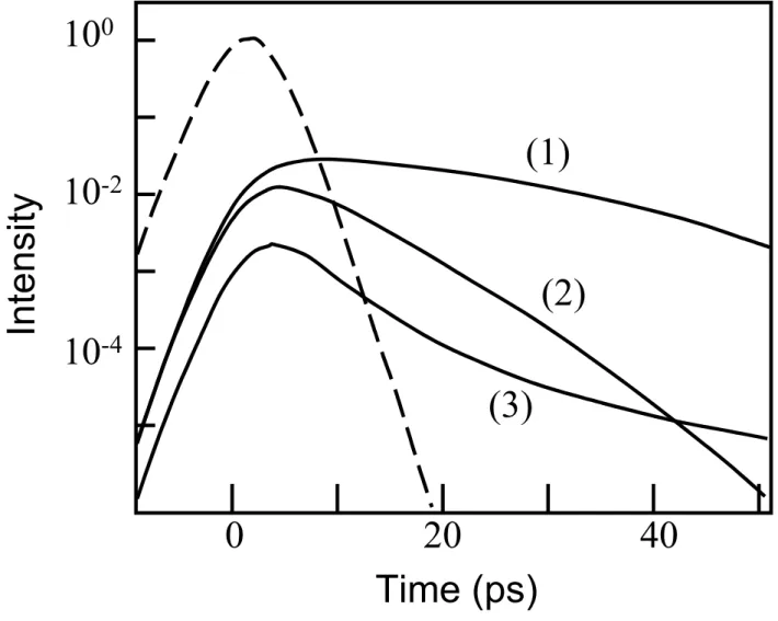
An effective method of THz pulses shaping, based on dispersive passage through a segment of metallic waveguide, was demonstrated by Mc Gowan, Gallot and Grischkowsky [1999]. In their experiment the pulses were coupled into the circular metal waveguide through a silicon lens and coupled out with a second silicon lens. The ~1 ps input pulse was stretched to 70 ps while propagation through the waveguide segment, equal to 80 initial pulse spatial lengths. The waveguide propagation is characterized by a multimode behavior and late time oscillations; the typical envelope of these oscillations in the outcoming pulse based on the measurements made by Mc Gowan, Gallot and Grischkowsky [1999], is shown on Fig. 10.

It is noticeable that a similar waveform can be obtained by means of direct time domain solutions of Maxwell equations for hollow circular waveguide with perfectly conducting walls. Let us consider the simplest axisymmetrical vortical TE01 mode in this waveguide, with Eϕ, Hρ

and Hz components. The component Eϕ is known to obey the wave equation

0 1 1 2 2 2 2 2 2 2 2 = ∂ ∂ − ∂ ∂ + − ∂ ∂ + ∂ ∂ t E c z E E E E_{ϕ ϕ ϕ ϕ ϕ} ρ ρ ρ ρ (2.59) Setting E_ϕ in a form: