HAL Id: hal-01140007
https://hal.archives-ouvertes.fr/hal-01140007
Submitted on 7 Apr 2015HAL is a multi-disciplinary open access
archive for the deposit and dissemination of sci-entific research documents, whether they are pub-lished or not. The documents may come from teaching and research institutions in France or abroad, or from public or private research centers.
L’archive ouverte pluridisciplinaire HAL, est destinée au dépôt et à la diffusion de documents scientifiques de niveau recherche, publiés ou non, émanant des établissements d’enseignement et de recherche français ou étrangers, des laboratoires publics ou privés.
Towards holographic spintronics
Koji Hashimoto, Norihiro Iizuka, Taro Kimura
To cite this version:
Koji Hashimoto, Norihiro Iizuka, Taro Kimura. Towards holographic spintronics. Physical Review D, American Physical Society, 2015, 91, pp.086003. �10.1103/PhysRevD.91.086003�. �hal-01140007�
Towards holographic spintronics
Koji Hashimoto,1,2,*Norihiro Iizuka,1,3,† and Taro Kimura4,2,‡ 1Department of Physics, Osaka University, Toyonaka, Osaka 560-0043, JAPAN 2Mathematical Physics Laboratory, RIKEN Nishina Center, Saitama 351-0198, JAPAN
3Yukawa Institute for Theoretical Physics, Kyoto University, Kyoto 606-8502, JAPAN 4Institute de Physique Théorique, CEA Saclay, 91191 Gif-sur-Yvette, FRANCE
(Received 5 May 2013; published 6 April 2015)
We study transport phenomena of total angular momentum in holography, as a first step toward holographic understanding of spin transport phenomena. Spin current, which has both the local Lorentz index for spins and the space-time vector index for current, couples naturally to the bulk spin connection. Therefore, the bulk spin connection becomes the source for the boundary spin current. This allows us to evaluate the spin current holographically, with a relation to the stress tensor and metric fluctuations in the bulk. We examine the spin transport coefficients and the thermal spin Hall conductivity in a simple holographic setup.
DOI:10.1103/PhysRevD.91.086003 PACS numbers: 11.25.Tq, 85.75.-d, 75.76.+j
I. INTRODUCTION
Spintronics is a technology where we manipulate the intrinsic electron spin degrees of freedom instead of the electric charge [1,2]. In ferromagnetic/antiferromagnetic materials, spin-charge separation can occur, and in such a situation, it is useful to consider spin as an independent degree of freedom which carries information. Because electric charge transport is not involved there, spin devices can reduce power consumption compared to usual electric ones and exceed the velocity limit of the electron charge. This spintronics is actually used widely, for example, for read heads of hard drives, and is based on a recent development of experimental technologies manipulating imbalance between up spins and down spins. For these reasons, spin transport phenomena have been attracting special interest recently.
Recent research on the spin transport basically relies on one-body quantum mechanical analyses, especially in the presence of a spin-orbit interaction. However, in strongly correlated systems, we have to go beyond the one-body physics by treating the interaction effect seriously. In this paper, we propose a method to study the spin transport phenomena for strongly correlated systems by using the holography, i.e., gauge/gravity correspondence [3–5]. The method of holography is one of the most useful tools to study strongly correlated quantum field theories. While there are some attempts to include effects of spins in holography, e.g., Refs.[6–14], study of spin transport itself has not yet been performed in the literature. To discuss the spin degrees of freedom, we first show a definition of spin current from a relativistic field theoretical viewpoint as a
conserved Nöther’s current. Then with this definition, we show how to deal with the spin transport coefficients from the holographic viewpoint. The key point is that the spin connection is naturally regarded as a source for the spin current. We demonstrate a holographic treatment of the spin transport, on a “boosted” Schwarzschild black brane back-ground in anti-de Sitter (AdS), and we calculate a spin transport coefficient and a thermal spin Hall conductivity.
II. SPIN CURRENT
The spin current is, as the name suggests, a flow of the intrinsic spin degrees of freedom, instead of the electric charge. If z-spin is conserved, namely a good quantum number, we can apply a naive definition of the spin current,
~Jz¼1
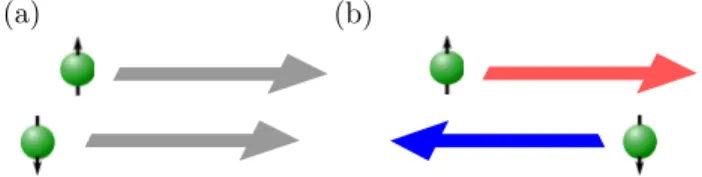
2ð~J↑− ~J↓Þ: ð1Þ This means that the spin current is given by the difference between flows of up and down spins, ~J↑ and ~J↓, while the electric current is the total contribution of them, ~J ¼ ~J↑þ ~J↓, as shown in Fig. 1. This definition (1)
FIG. 1 (color online). (a) The charge current is just the total contribution of up- and down-spin currents ~J ¼ ~J↑þ ~J↓.
(b) The spin current is given by difference between them, ~Jz¼12ð~J↑− ~J↓Þ. This picture is available if and only if
z-direction spin is conserved.
*[email protected]‑u.ac.jp †[email protected]‑u.ac.jp ‡[email protected]
PHYSICAL REVIEW D 91, 086003 (2015)
corresponds to the Schwinger representation of the spin operator, ~s ¼1
2ψ†~σψ.
The expression(1)is available if and only if the spin is conserved or, at least, approximately conserved [15]. However, generically the electron spin is not conserved by itself, due to the spin-orbit interaction. Therefore, the naive definition of the spin current(1)has to be modified in the presence of such an effect.
First we consider how to define the spin current from the field theoretical point of view. Let us recall the treatment of conserved currents in the context of quantum field theories. A conserved current is defined as a variation of an action with respect to the corresponding source. For example, the electric current Jμ is derived by differentiating an action with respect to a U(1) gauge field,
Jμ¼ δS δAμ
: ð2Þ
Conservation of Jμ is guaranteed by Nöther’s theorem, associated with a U(1) gauge symmetry,
∂μJμ¼ 0: ð3Þ
In the weak coupling limit of a U(1) gauge theory, the U(1) local symmetry reduces to a global one. The Aμbecomes a nondynamical background gauge potential, which is a source, and the Jμ becomes a global current. In this limit, the global U(1) current Jμ couples to the source A
μin the Lagrangian as Lsource¼ AμJμ. Therefore, the U(1) current Jμ is obtained by differentiating the action with respect to its source Aμ.
Similarly a stress tensor is given by a variation of an action with respect to a metric,
Tμν¼ 1 ffiffiffiffiffiffi −g p δgδS μν : ð4Þ
The conservation of energy and momentum
∂μTμν¼ 0 ð5Þ
comes from the translation invariance in temporal and spatial directions, respectively. In the weak gravity limit (where gravity is decoupled), nondynamical background metric gμν becomes a source for the stress tensor, and it couples with the stress tensor as Lsource¼ gμνTμν in the Lagrangian.
In this way, in order to obtain a conserved quantity, we have to introduce a corresponding field (or source) which couples to the conserved quantity. For the case of the spin current Jμ
ˆ
a ˆb, our claim is that the spin connection ωμa ˆbˆ is the corresponding field (source). This implies that they couple as Lsource ¼ ωμa ˆbˆ Jμa ˆbˆ in the Lagrangian. By differ-entiating an action with respect to the spin connection, we can obtain the spin current.
To see why it is so, let us recall the nature of spin. The spin operator saˆ ¼ σaˆ=2 has an index ˆa for the orientation of the spin. Here the hatted index ˆa takes only a spatial coordinate as ˆa ¼ ˆx; ˆy; ˆz, and σ is the Pauli matrix. Spin is conserved only in the sense that the total angular momen-tum is conserved. The total angular momenmomen-tum is asso-ciated with the global rotational symmetry of the system. If we uplift this global rotational symmetry to a local one, then these become a subgroup of the local Lorentz symmetry. Therefore, it is natural to associate the conserved spin σaˆ to a local Lorentz generator Σa ˆbˆ ¼4i½γaˆ; γˆb& as σaˆ ¼ ϵa ˆb ˆcˆ Σ
ˆb ˆc, where ϵa ˆb ˆcˆ is an antisymmetric tensor taking '1 defined on the spatial part of the local Lorentz indices; i.e., ˆa; ˆb; ˆc of ϵa ˆb ˆcˆ takes only ˆx; ˆy; ˆz. Furthermore, since the spin connection ωμa ˆbˆ is a gauge field associated with the local Lorentz symmetry, it is natural to associate it to the conserved spin current Jμ
ˆ a ˆb, as Eq.(2).
Therefore, we reach a conclusion that a spin current is given by a variation of an action with respect to a spin connection as Jμ ˆ a ˆb¼ δS δωμa ˆbˆ : ð6Þ
From now on, the hatted indices ˆa; ˆb; … represent the local Lorentz indices, so they stand for ˆt; ˆx; ˆy; ˆz. Greek indices μ; ν; … stand for curved spacetime vector indices. The spin connection is written in terms of a vielbein eμaˆ as
ωμa ˆbˆ ¼ eνaˆ∇μeν ˆb¼ eνaˆ∂μeν ˆbþ eλaˆΓλμνeν ˆb
¼ −eνˆb∇μeν ˆa¼ −ωμˆb ˆa; ð7Þ where Γλ
μν stands for the Christoffel symbol, and the vielbein eμaˆ satisfies gμν¼ ηa ˆbˆ eμaˆeνˆb, with the local Lorentz metric ηa ˆbˆ ¼ diagð−1; 1; 1; 1Þ.
Usually, we call the following current as a spin current, Jμ ˆa¼ ϵˆ0 ˆa ˆb ˆcJμ
ˆb ˆc; ð8Þ
rather than the former one Jμ ˆ
a ˆb. Here we use the con-vention ϵˆ0 ˆ1 ˆ2 ˆ3¼ 1. One can easily see that the definition(8)
is consistent with, for example, the standard free fermion spin current. To see this, let us consider the generic form of a fermionic Lagrangian on a curved space, which is given by LF ¼ ¯ψ " ieμ ˆ aγaˆ # ∂μ− iAμ−i 2ωμ ˆ a ˆbΣ ˆ a ˆb $ − m % ψ: ð9Þ From this, we have the spin current by differentiating it with the spin connection,
Jμ ˆ a ˆb¼ 1 2ψγ¯ μΣ ˆ a ˆbψ⟶Jμaˆ ¼1 2ψγ¯ μðσ ˆ a⊗ 1Þψ: ð10Þ This is regarded as a current carrying ˆa-direction spin. We can see that the zeroth component correctly gives the spin density
J0 ˆ
a¼ ψ†ðsaˆ ⊗ 1Þψ: ð11Þ In this way, we have seen that the definition(8)is consistent with the conventional one for the spin current. However, it is more convenient to consider Jμ
ˆ
a ˆbas a spin current, since Jμ
ˆ
adefined in Eq.(8)is not local Lorentz invariant tensor. This is because the ϵˆ0 ˆa ˆb ˆc tensor takes explicit index component ˆ0.
The conservation of the spin current Jμ ˆ a ˆb,
∂μJμa ˆbˆ ¼ 0; ð12Þ is associated with the local Lorentz invariance, and the spin current Jμ
ˆ
a ˆb couples to the source term ωμa ˆbˆ in the Lagrangian as Lsource¼ ωμa ˆbˆ Jμa ˆbˆ .
Precisely speaking, what we define above is “total angular momentum” current, rather than “spin” current. Note that only the total contribution of the angular momentum current, coming from both the orbital and the spin angular momentum, is conserved. A difficulty in dealing with spin transport phenomena is in the definition of the spin current, because the intrinsic spin is not conserved solely but rather conserved as a whole angular momentum. Therefore, the spin current, by itself, cannot be introduced as a conserved Nöther current at least in the relativistic limit. Thus, in this sense, the spin current defined above is slightly different from the conventional definition of the spin current often used in the nonrelativ-istic condensed-matter system, which includes the contri-bution of only the intrinsic electron spin.
We will also point out that it is possible that the orbital contribution gives only a subleading contribution, in the nonrelativistic limit. This is because the orbital angular momentum includes the spatial momentum as ~L ¼ ~x × ~p. Thus, by taking an appropriate limit, the spin current, defined as a conserved one, may provide a good description of the spin transport. We will discuss how we take the nonrelativ-istic limit a bit more in detail in the discussion later.
There is a number of attempts to define the spin current in the literature. The original idea of using the spin connection as a source to obtain a spin current is found in Refs. [16,17], especially in 2 þ 1 dimensions. In
Ref.[16]the authors treated the space and time separately and broke the Lorentz invariance explicitly. Another attempt to define a spin current is performed by introducing an SU(2)-valued gauge field, coupled to a spin degrees of freedom, in addition to a U(1) electromagnetic field
[18–20]. This SU(2) symmetry can be seen as a remnant
of the local Lorentz symmetry, which is decomposed as SOð1; 3Þ ≅ SUð2Þ × SUð2Þ in 3 þ 1 dimensions. However, since these SU(2) are not decoupled except for the massless case, it is difficult to define the spin current as a conserved current only with the SU(2) gauge field. Actually, this SU(2) symmetry is broken in the presence of the spin-orbit interaction.
III. HOLOGRAPHY
Given the spin current definition in terms of spin connection, in order to study the spin current by the gauge/gravity duality scheme, we will evaluate the fluc-tuation mode of the spin connection. Note that holography induces one extra coordinate, i.e., a radial direction. So in the gravity side, the local Lorentz index runs as ˆ
a ¼ ˆt; ˆx; ˆy; ˆz and ˆr. Similarly the vector index runs μ ¼ t; x; y; z; r.
Before studying a component of the spin connection corresponding to a spin current in a spatial direction, we analyze a temporal component of a spin current Jtx ˆyˆ , as an example. This term couples to ωtx ˆyˆ . When the background metric is diagonal, the static contribution is calculated as
δωtx ˆyˆ ¼1 2e
xˆxeyˆy
ð∂yδgtx−∂xδgtyÞ: ð13Þ Here we apply a gauge choice eraˆ≠ˆr ¼ grμ≠r¼ 0. From the indices, it is clear that this represents a rotation of a metric fluctuation in the xy-plane. In terms of the gauge/gravity duality, the non-normalizable mode of this component is regarded as a chemical potential for the ˆz-component of the total angular momentum, i.e., ωx ˆyˆ
tðNNÞ¼12μ ˆ
z, where the index (NN) represents the non-normalizable mode [21]. This chemical potential is naively interpreted as the difference between those for up and down spins, μˆz¼1
2ðμ↑− μ↓Þ. The ˆz-component spin density Jt ˆ z cor-responds to the normalizable mode of ωx ˆyt ðNÞˆ in the holo-graphic viewpoint, where the index (N) represents the normalizable mode.
Similarly, let us study a fluctuation of the spin con-nection along the x-spatial direction, ωxx ˆyˆ . This corre-sponds to a spin current Jxx ˆyˆ ¼12Jx
ˆ
z; i.e., ˆz-oriented spin flows along the x direction. Here we can see that we need to turn on some of the off-diagonal elements of the back-ground metric, in particular gtx and gty, which correspond to nonvanishing off-diagonal contributions of vielbeins, etxˆ and etyˆ. To see this, assuming that the fluctuation depends only on r and t directions, we obtain
δωxx ˆyˆ ¼ −1 2e tˆxeyˆy∂ tδgxyþ1 2e xˆxetˆy∂ tδgxx: ð14Þ From this expression one can see that the off-diagonal components of the metric, etˆx and etyˆ, or equivalently gtx
TOWARDS HOLOGRAPHIC SPINTRONICS PHYSICAL REVIEW D 91, 086003 (2015)
and gty, are required in order to give the spin current Jxzˆ. A physical meaning of this condition is discussed later.
IV. EXAMPLE: “BOOSTED” BLACK BRANE So far we have considered a boundary theory in 3 þ 1 (ˆx; ˆy; ˆz and ˆt) dimensions. However, even if the boundary theory is 2 þ 1 dimensional, none of our argument so far is modified since 2 þ 1-dimensional theories still admit a spin along the “z”-direction; Here z-direction is simply the ðˆa; ˆbÞ ¼ ðˆx; ˆyÞ component, Jμx ˆyˆ . We will conduct a cal-culation of the spin current in a holographic setting, but for simplicity of the calculation in the bulk, we consider a bulk theory in 3 þ 1 dimensions, which corresponds to a boundary theory in 2 þ 1 dimensions.
We demonstrate a calculation of the transport coeffi-cients for spin with the simplest holographic setup, i.e., pure gravity in 3 þ 1 dimensions,
S ¼ Sbulkþ Sboundary; ð15Þ Sbulk¼ Z d4x ffiffiffiffiffiffip−g ðR½g& − 2ΛÞ; ð16Þ Sboundary¼ 2 Z d3x ffiffiffiffiffiffip Θ;−γ ð17Þ where the cosmological constant is Λ ¼ −3, and γμνis the boundary metric, defined by the metric components along the boundary dimensions. Θ is a scalar defined with the extrinsic curvature Θμν¼ −1
2ð∇μnνþ ∇νnμÞ, as Θ ¼ γμνΘμν. nμ is outward unit vector pointing along the radial direction. This boundary action is to provide a well-defined Dirichlet variational principle. In addition, we have to also take into account another counterterm, called the cosmological counterterm, which depends on the intrinsic curvature of the boundary[22]. Although this counterterm is important for the regulation of the boundary stress tensor, it is known that the correct boundary stress tensor, involving the contribution from the cosmological counter-term, can be read off simply from the normalizable modes of the metric[23]. As explained later, we will study the spin current in terms of the stress tensor based on the relation between the spin connection and the metric, and further-more we will read off the boundary stress tensor from the normalizable modes. Therefore, we just apply the argument for the stress tensor, instead of taking the variation with the spin connection without worrying about the cosmological counterterm.
We study metric fluctuations around a boosted Schwarzschild black brane solution in AdS4,
ds2 ¼ −UðrÞdt2 þUðrÞ1 dr2 þ r2dy2 þ ðr2− a2UðrÞÞdx2− 2aUðrÞdtdx; ð18Þ with UðrÞ ¼ ðr3− r3
0Þ=r. r ¼ r0 is the horizon while r ¼ ∞ is the boundary. r0 is related to the temperature T as T ¼ 3r0=4π [24]. This metric was obtained by a coordinate transformation t → t þ ax on the AdS-Schwarzschild solution, and it suffices for our purpose since it includes the off-diagonal metric element gtx. We can check that this satisfies the Einstein equation Rμν−12gμνR þ Λgμν¼ 0 and is not singular for jaj < 1, and we can consider a > 0 without loss of generality.
Let us perform a fluctuation analysis around the back-ground solution. Fluctuations we consider are δgtyand δgxy, and we assume the following form for ac fluctuations,
δgty¼ δgyt¼ ϵ e−iωtr2fðrÞ; ð19Þ δgxy¼ δgyx¼ ϵ e−iωtr2hðrÞ: ð20Þ Then, nontrivial components of the Einstein equation to linear order in these fluctuations, OðϵÞ, are found to be just the ty-component, the ry-component and the xy-component. The other components of the Einstein equation turn out to be trivially satisfied. Among the three equations, the ry-component provides a constraint,
f0ðrÞ ¼ # a þaðr3r3 0− r3Þ $−1 h0ðrÞ; ð21Þ where 0 is for the r-derivative. With this relation, the ty-component reduces to a simple equation solely for hðrÞ, hðrÞ þr3− r30 ω2r3 d dr " ðr3− r3 0Þr4 ð1 − a2Þr3þ a2r3 0 d drhðrÞ % ¼ 0: ð22Þ Furthermore, the remaining xy-component of the Einstein equations also reduces to the same equation (22). So, we just need to solve the equation(22)for hðrÞ and relate it to
fðrÞ via the constraint equation(21). This equation(22), in the limit a ¼ 0, coincides with the equation for the shear viscosity calculation[25,26].
Equation (22) can be written by a new coordinate x≡ r0=r as ω2 r2 0 hðxÞ ¼ x2 ðx3− 1Þ d dx " 1− x3 x2 ð1 − a2 þ a2x3 Þ dhðxÞ dx % : ð23Þ The new coordinate x ranging 0≤ x ≤ 1 can make the boundary analysis easier.
Near the horizon x ¼ 1, we can solve (23)as h∝ exp # −i 3 ω r0logð1 − xÞ $ ; ð24Þ
which amounts to the ingoing boundary condition at the horizon. Note that the equation of motion (23) and the ingoing boundary condition(24)depend on r0only through
the combination ω=r0. Since T∝ r0, the temperature dependence is the same as the 1=ω dependence. This is because the background is a finite temperature system of an AdS space, namely a scale invariant system, and therefore any nontrivial dependence comes from only the dimension-less ratio, ω=r0 [27].
Near the boundary x ¼ 0, we have two independent solutions of(23), h ¼ h0 # 1−1 2γx 2−1 8γ 2x4 þ ( ( ( $ ; ð25Þ h ¼ h3ðx3þ ( ( (Þ; ð26Þ with γðω; TÞ ≡ ð1 − a2 Þω2=r2
0. Here h0 and h3 are integration constants. We can find that h0 is the non-normalizable mode, while h3 is the normalizable mode. Consider the bulk action, Eq.(16), and expand that around r →∞ in the background equation (18), with the fluc-tuation hðrÞ and fðrÞ. After using the constraint(21), we find, to the quadratic order in hðrÞ, the leading r behavior of the Einstein action is
ffiffiffiffiffiffi −g p ½R½g& − 2Λ&jr→∞ ¼ ðbackgroundÞ −ϵ 2e−2iωtr4 2ð1 − a2Þh0ðrÞ 2; ð27Þ
neglecting the boundary terms. From this expression, we confirm that h∼ const is the non-normalizable mode[28], while h∼ r−3 is the normalizable mode.
We can also specify the boundary condition for the other fluctuation fðrÞ. From(21), we obtain
fðxÞ ¼ Z x 1 aðs3− 1Þ a2s3− a2 þ 1 dhðsÞ ds ds þ c; ð28Þ where c is an integration constant. Near the horizon x ¼ 1, hðxÞ approximated as (24) can give an ingoing wave for fðxÞ only if c ¼ 0. So we need to put c ¼ 0, and fðxÞ is uniquely determined once hðxÞ is given. The magnitude f0 of the non-normalizable mode of fðxÞ can be read by(28)
with c ¼ 0, while the magnitude h3 of the normalizable mode of fðxÞ is proportional to that of hðxÞ (which is h3), through(28).
V. SPIN CURRENT AND STRESS TENSOR Let us pose and understand the physical meaning of the modes we consider above. The spin connection can be written with the metric, or the vielbein as Eq. (7). This means that the spin current, which is dual to the spin connection, should be associated with the stress tensor, which is dual to the metric. Therefore, we have to evaluate
the spin current by taking into account its relation to the stress tensor. In other words, the spin current can be determined by comparing the coefficients appearing in the following relation:
Jμ ˆ
a ˆbδωμa ˆbˆ ¼ Tρσδγρσ ¼ δL: ð29Þ
Here L is the Lagrangian of the quantum field theory in the boundary 2 þ 1 dimensions. Note that these metric and spin connections are defined on the boundary, and therefore all the indices run without the radial direction. We have omitted the volume factorpffiffiffiffiffiffi−γ for simplicity.
To obtain an explicit relation between the spin current and the stress tensor, we first need to choose a local Lorentz frame. Any spin current is dependent on the choice of the frame. The boundary metric is
gtt¼ −1; gtx¼ gxy¼ −a; gxx¼ 1 − a2; gyy¼ 1: ð30Þ These are given by subtracting the scale factor r of the bulk metric in the limit r →∞. A natural choice of the local Lorentz frame for the background vielbein consistent with this metric is given by[29]
etˆt¼ 1; exˆt¼ a; exxˆ¼ 1; eyyˆ¼ 1: ð31Þ We turned on the ac fluctuation of the metric given by Eqs. (19) and (20), and the most generic vielbein fluctuation consistent with (19) and (20) is a set fetyˆ; exyˆ; eyˆt; eyxˆg, which satisfies the two relations
etyˆ− eyˆt¼ ϵ e−iωtþikxxþikyyf0; ð32Þ
exyˆþ eyxˆ− aeyˆt¼ ϵ e−iωtþikxxþikyyh0 ð33Þ coming from the constraint γμν¼ eμaˆeνˆbηa ˆbˆ . Here we used Fourier modes as ∼e−iωtþikxxþikyy, and ðω; kx; kyÞ is the
frequency/momentum for the fluctuations. The other com-ponents of the vielbein are consistently put to zero in our case.
With this at hand, all nontrivial components of the spin connection are
TOWARDS HOLOGRAPHIC SPINTRONICS PHYSICAL REVIEW D 91, 086003 (2015)
δωtˆt ˆy¼ iωeyˆt; δωtx ˆyˆ ¼ −i 2kxðet ˆ y− e yˆtÞ þi 2ωðey ˆ x− e xˆyþ aeyˆtÞ; δωxˆt ˆy¼ −i 2kxðet ˆ y þ eyˆtÞ þi 2ωð−ey ˆ x− e xyˆþ aeyˆtÞ; δωxx ˆyˆ ¼ −i 2kxð2ey ˆ xþ ae tyˆ− aeyˆtÞ þ2iaωð−eyxˆ− exyˆþ aeyˆtÞ; δωyˆt ˆx¼ −i 2kxðet ˆ y− e yˆtÞ þi 2ωð−ey ˆ x− e xyˆþ aeyˆtÞ; δωyˆt ˆy¼ −ikyetyˆ;
δωyx ˆyˆ ¼ −ikyðaetyˆ− exyˆÞ: ð34Þ Keeping the two relations(32) and(33)satisfied, we can make a gauge choice of the local Lorentz frame, eyˆt¼ eyxˆ¼ 0, and restrict ourselves to homogeneous fluctuation, kx¼ ky¼ 0. In this local Lorentz frame, the above spin connections are simplified, and all the nonzero components are δωxx ˆyˆ ¼ − iaω 2 ϵ e −iωth 0; ð35Þ
δωtx ˆyˆ ¼ δωxˆt ˆy¼ δωyˆt ˆx¼ −iω 2 ϵ e
−iωth
0: ð36Þ Since h0is the constant mode of the boundary metric gxy, it is a source for the boundary stress tensor Txy, and therefore we obtain the spin current coupled to the spin connection from this expression as
Jxx ˆyˆ ¼ −1a 1 2iωT xy; ð37Þ Jtx ˆyˆ ¼ Jxˆt ˆy¼ Jyˆt ˆx¼ − 1 2iωT xy: ð38Þ All the other components, other than each antisymmetric partner Jμˆb ˆa¼ −Jμa ˆbˆ , are zero. These combined with(35) and(36)clearly satisfy(29). Jx ˆyxˆ is the spin current along the x direction, and Jtx ˆyˆ ð¼ Jxˆt ˆy¼ Jyˆt ˆxÞ is the temporal component of the spin current, corresponding to the spin density.
Here we have employed a choice of the local Lorentz frame eyˆt¼ eyˆx¼ 0. However, other local Lorentz frame choices are also possible. Actually, for a certain other choice of the local Lorentz frame, one can show that the spin current determined in this way is equivalent to a popular definition of the angular momentum current M made by the stress-energy tensor,
Mμ
νλ≡ xνTμλ− xλTμν: ð39Þ
Due to this relation, for example, we can obtain the normalizable and non-normalizable modes for the spin connection from those for the metric. Note that this current is with the target spacetime indices, so in order for this to be equivalent to our spin current J, a certain local Lorentz frame should be appropriately chosen.
To check this explicitly, we consider our case of nonzero Tty and Txy. We consider a ¼ 0 for simplicity. From the definition(39), one obtains
Mt ty¼ −tTty; Mtxy¼ xTty; Mxty¼ −tTxy; Mx xy¼ xTxy; Mytx¼ xTty− tTxy; My ty¼ yTty; Myxy¼ −yTxy: ð40Þ
One can show that all of these are consistent with the spin connections (34) only when we choose a local Lorentz frame at which
etyˆ¼ −eyˆt; exyˆ¼ eyxˆ ð41Þ are satisfied. To see this, in this case,(32)and(33)become
etyˆ ¼ −eyˆt¼1 2ϵ e −iωtþikxxþikyyf 0¼ 1 2δgty; ð42Þ exyˆ ¼ eyxˆ ¼1 2ϵ e−iωtþik xxþikyyh 0¼ 1 2δgxy; ð43Þ and(34)becomes δωtˆt ˆy¼1 2∂tδgty; δωt ˆ x ˆy ¼ −12∂xδgty; δωxˆt ˆy¼ 1 2∂tδgxy; δωx ˆ x ˆy¼ −1 2∂xδgxy; δωyˆt ˆx¼ −1 2∂xδgtyþ 1 2∂tδgxy; δωyˆt ˆy¼ −1 2∂yδgty; δωy ˆ x ˆy ¼12∂yδgxy: ð44Þ Therefore, the angular momentum current Mμ
νλ given by (40) satisfies our previous anticipation (29) with the spin connection(44)via a partial integration.
The freedom for the local Lorentz frame choice corre-sponds to the freedom for the local choice of the axes to define the rotation for the angular momentum. Note that in any choice of the local Lorentz frame for the vielbein fluctuations, interestingly, the expression of the most important spin connection(35)is universal, and therefore so is(37).
VI. TRANSPORT COEFFICIENTS
h3is proportional to the spin current Jxzˆ¼ 2Jxx ˆyˆ . h0is proportional to the spin gradient along the x direction∇xμˆz,
because ∇xμzˆ¼ 2∇xωt ðNNÞˆx ˆy is gauge equivalent to −2∇tωx ðNNÞx ˆyˆ ¼ 2iω ωx ðNNÞx ˆyˆ .
f0 corresponds to the thermal gradient along the y direction due to the relation iωδgðNNÞty ¼ r2∇yT=T [30]. f3corresponds to a thermal current along the y direction, since δgðNÞ
ty is dual to the stress tensor, δgðNÞty ¼ Tty. From these, we can evaluate the spin transport coefficient α and the thermal spin Hall conductivity κsH, defined as
Jxzˆ¼ −α∇xμˆz; Jxzˆ¼ −κsH∇yT: ð45Þ Using holography, these coefficients are represented by normalizable and non-normalizable modes as
α ¼ − Jx ˆ x ˆy iωδωx ˆyˆ x ðNNÞ ¼ia2hω33h 0 ; ð46Þ κsH¼ − 2Jxx ˆyˆ iωTδgðNNÞ ty =r2 ¼ −aωh2Tf3 0 : ð47Þ
As we have seen, the ratio h3=h0and h3=f0are functions of only ω=T, in Eqs.(23),(24)and(28). We obtain these by solving the bulk equation and imposing the ingoing boundary condition at the horizon, and the radial r dependence of the bulk equation is reflected as ω=r0 dependence in the boundary viewpoint.
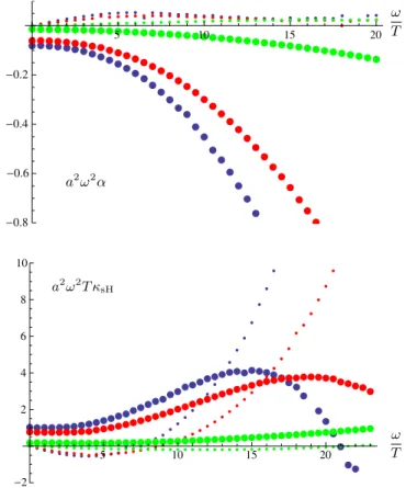
Actually the sources ðh0; f0Þ and the expectation values ðh3; f3Þ are related by a 2 by 2 matrix, and the coefficients α and κsH are just the upper two elements of this 2 by 2 matrix. However, as we have seen, in our system it follows that f3¼ ða − 1=aÞ−1h3due to the relation(21), where f3 is the normalizable mode coefficient for fðrÞ, just as h3in the equation(26). Therefore, the ratio f3=f0 and the ratio f3=h0are essentially the same as h3=f0and the ratio h3=h0. We have evaluated these transport coefficients by a numerical method for solving the differential equation(23). By varying the frequency ω, we find the ac conductivities as shown in Fig. 2 [31].
For the numerical simulations, we have worked in the unit T ¼ 1 and chosen a ¼ 0.03, a ¼ 0.5 and a ¼ 0.9 for simplicity. The top figure of Fig. 2 is the spin transport coefficient α. This is the coefficient on the spin current Jxzˆ as a response to the ac external gradient of the spin chemical potential μzˆ. The bottom figure of Fig. 2is the thermal spin Hall conductivity κsH. In both figures, the transport coefficients are multiplied by a2ω2 to show the ω=T dependence clearly. From the figures, we find that the imaginary parts ×ω2 vanish linearly at ω ¼ 0, so around the origin the imaginary parts behave as 1=ω. This means that in the real parts there exists a Drude peak proportional to δðωÞ often observed in superconducting/ metal phases. We also see specific behavior of the thermal spin Hall conductivity, changing the sign of the transport
coefficient as the frequency gets larger. It is quite interest-ing to observe such frequency dependence by experimental or other theoretical setups.
VII. ON THE SPIN CURRENT DEFINITION We have evaluated the spin current following the relation
(29). However, (29) is not necessarily the same as our definition of the spin current(6). We will now discuss that the spin current evaluated by the definition(6)yields zero value, using the action(15) [32]. This is the reason why we need to relate the spin current to the stress tensor as(29), which we have used in this paper.
To obtain the spin current following the definition(6)in holography, note that (6) means that we have to differ-entiate the action(15)with the boundary spin connection, which is defined by the spin connections along the boundary directions. The contribution coming from a variation of the bulk action (16) by the boundary spin connection, vanishes by using the bulk equations of motion. Thus, the contribution to the spin current comes from a variation of the boundary action(17)only. However, we will see that this contribution also vanishes.
FIG. 2 (color online). Top: the spin transport coefficient α as a function of the frequency over the temperature, ω=T. Large dots are the real part Re½α&, and small dots are the imaginary part Im½α&. Blue, red and green correspond to a ¼ 0.03, 0.5 and 0.9, respectively. Bottom: the thermal spin Hall conductivity κsHas a
function of ω=T.
TOWARDS HOLOGRAPHIC SPINTRONICS PHYSICAL REVIEW D 91, 086003 (2015)
Whenever we take a variation, we have to fix all the other quantities. In this case, we regard each of the boundary spin connection components as an independent degree of free-dom, and then we take a variation of the action by that, while keeping all the other quantities, which include the metric, fixed. In this formulation, each spin connection component is an independent degree of freedom from the metric; the independent degrees of freedom are metric and spin connection. In fact, we can formulate general relativity in such a way, by i.e., the so-called Palatini formulation of gravity. However, this procedure turns out to give a vanishing spin current.
To see this, let us conduct a variation of the boundary action(17)by the boundary spin connection. The extrinsic curvature Θ is written with the normal vector nμ as Θ ¼ −γμν∇
μnν. In the Palatini formalism, the boundary metric γμνand the boundary spin connection are indepen-dent, and therefore the contribution form the boundary action variation yields
Jμ ˆ a ˆb¼ −2γρσ δΓηξλ δωμa ˆbˆ δð∇ρnσÞ δΓη ξλ ¼ −2e μ ˆ aeνˆbnν: ð48Þ
Since nν≠ 0 only when ν ¼ r and erˆb≠ 0 only when ˆb ¼ ˆr, there is no spin current on the boundary. This shows that the spin current evaluated by the Palatini formalism vanishes [33]. To obtain a nonvanishing spin current, we should not regard the metric and the spin connection as independent degrees of freedom. We need to modify our definition of the spin current (6)slightly.
Therefore, in this paper we do not regard the spin connection as an independent variable but associate it with the metric. This further implies that our spin current, which is dual to the spin connection, should be associated with the stress tensor, which is dual to the metric. In the Palatini formalism, the relation (7) comes from the equation of motion for the spin connection. Therefore, we have evaluated the spin current by taking into account its relation to the stress tensor as (29)in this paper.
VIII. DISCUSSIONS : SPIN VS ANGULAR MOMENTUM
In this paper we have investigated the spin transport phenomena from the viewpoint of gauge/gravity corre-spondence. We have introduced the proper definition of the spin current, as a conserved Nöther’s current, which couples naturally to the spin connection.
We have analyzed the AdS Schwarzschild black brane geometry as a simple example to demonstrate how to study the spin transport in the context of the holography. We have calculated the spin transport coefficient α and the thermal spin Hall conductivity κsH by studying the fluctuations of the metric components. We have obtained the corresponding transport coefficient from the
non-normalizable and normalizable modes propagating in the bulk gravity.
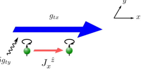
Let us comment on a physical meaning of the holo-graphic analysis done in this paper. We have seen that the off-diagonal metric component for the background, i.e., gtxð¼ gxyÞ, is required for giving the spin current. Note that if there is such a component in the background geometry that leads to a constant energy flow coupled to gtx. By applying the fluctuation δgtyin addition to the background flow, we should have an angular momentum current in the x-direction as shown in Fig.3. It seems that our spin current almost corresponds to the orbital part of the angular momentum.
However, at least from the relativistic theoretical view-point, we cannot split the total angular momentum into contributions from orbital and intrinsic spin; spin is originally defined in the nonrelativistic system, where the Lorentz invariance is broken and we should treat space and time separately. Since in this paper we have considered the total angular momentum current defined in relativistic field theory, in order to really discuss the spin current, we need to take an appropriate nonrelativistic limit of our system. Only after taking that, we can extrapolate the spin contribution from the total angular momentum current, and we can discuss if the orbital contribution gives only a subleading contribution or not.
The nonrelativistic limit of relativistic conformal field theories is obtained by taking the discreet light-cone quantization (DLCQ). This limit reduces the boundary metric from AdS into the form[34–38]
ds2 ¼ −r2z ðdxþÞ2 þdr 2 r2 þ 2r 2dxþdx−þ r2d~x2; ð49Þ
where xþ is the light front time, and r is the holographic radial direction as before. x− is a new direction associated with the boost direction and we compactly x−∼ x−þ R, and has an interpretation as “dual” to the conserved particle number since P− is quantized as N=R, where N is the particle number. z is called the “dynamical exponent” and represents the difference of the scaling between time xþand spatial coordinate ~x.
FIG. 3 (color online). When the off-diagonal background metric gtx, namely a constant energy flow in the x-direction, is
turned on, the angular momentum current as a spin current Jxˆzis
For example, starting from a boundary theory which is 3þ 1 dimensional, we can obtain a 2 þ 1-dimensional nonrelativistic theory where we can identify xþ ¼ t þ x3 and x−¼ t − x3. This metric possesses the Schrödinger symmetry for the z ¼ 2 case.
Taking this DLCQ limit, or simply replacing the boun-dary metric from AdS into the above, is not enough for extracting the spin information, since spin is not a con-served quantity by itself even here, and only the total angular momentum is a conserved one. To eliminate the contribution of the orbital angular momentum, it is best to consider a setting where the momentum of the particle is suppressed, namely an insulator. The insulator is realized as a system which has an energy gap. The energy gap is reflected in a holographic setting in the bulk as a system which has an IR cutoff, like the confinement in holographic QCD. The hard wall model is the simplest setting to realize the mass gap, and therefore this would lead one to a system which has an asymptotic metric as(49)and has an IR cutoff. Such a bulk setup is good for us to study the spin-transport phenomena, and it is interesting to see how
the orbital and the real spin parts contribute to our total spin current, after taking the nonrelativistic limit.
In this paper we considered only the spin-current induction by the spin-current potential and also thermopo-tential, but not the one induced by an electric field. In real experiments, the spin current induced by some external electric field is more often considered, so this forces us to consider a bulk action coupled to the electromagnetic field. Adding impurity effects[7,13,39,40]is also important. We hope to return to these analyses in the near future.
ACKNOWLEDGMENTS
N. I. would like to thank RIKEN Mathematical Physics Laboratory for kind hospitality where this project started. The research of K. H. is supported in part by JSPS Grants-in-Aid for Scientific Research No. 23105716, No. 23654096, and No. 22340069. The research of T. K. is supported in part by Grant-in-Aid for JSPS Fellows (Grant No. 23-593).
[1] S. Maekawa (ed.), Concepts in Spin Electronics (Oxford University Press, New York, 2006).
[2] I. Žutić and H. Dery, Nat. Mater. 10, 647 (2011). [3] J. M. Maldacena, Adv. Theor. Math. Phys. 2, 231 (1998). [4] S. Gubser, I. R. Klebanov, and A. M. Polyakov,Phys. Lett.
B 428, 105 (1998).
[5] E. Witten, Adv. Theor. Math. Phys. 2, 253 (1998). [6] F. Benini, C. P. Herzog, R. Rahman, and A. Yarom,J. High
Energy Phys. 11 (2010) 137.
[7] S. Harrison, S. Kachru, and G. Torroba,Classical Quantum Gravity 29, 194005 (2012).
[8] F. Bigazzi, A. L. Cotrone, D. Musso, N. P. Fokeeva, and D. Seminara,J. High Energy Phys. 02 (2012) 078.
[9] C. P. Herzog and J. Ren,J. High Energy Phys. 06 (2012) 078.
[10] P. Benincasa and A. V. Ramallo, J. High Energy Phys. 06 (2012) 133.
[11] V. Alexandrov and P. Coleman, Phys. Rev. B 86, 125145 (2012).
[12] M. Luo,arXiv:1205.3267.
[13] K. Hashimoto and N. Iizuka,arXiv:1207.4643.
[14] T. Ishii and S.-J. Sin, J. High Energy Phys. 04 (2013) 128.
[15] For the spin to be approximately conserved, its coherence time must be sufficiently larger than its characteristic time scale.
[16] X. G. Wen and A. Zee,Phys. Rev. Lett. 69, 953 (1992). [17] J. Fröhlich and U. M. Studer, Rev. Mod. Phys. 65, 733
(1993).
[18] V. Mineev and G. Volovik, J. Low Temp. Phys. 89, 823 (1992).
[19] A. S. Goldhaber, Phys. Rev. Lett. 62, 482 (1989).
[20] J. Fröhlich and U. Studer,Commun. Math. Phys. 148, 553 (1992).
[21] The factor 1=2 is for a convenience due to the definition, Eq.(8).
[22] V. Balasubramanian and P. Kraus,Commun. Math. Phys. 208, 413 (1999).
[23] S. de Haro, S. N. Solodukhin, and K. Skenderis,Commun. Math. Phys.217, 595 (2001).
[24] Our “boost” is simply a coordinate transformation. Since it is different from the Lorentz boost, it does not involve the γ factor for a Lorentz transformation, and therefore the temperature does not change by this boost.
[25] P. K. Kovtun, D. T. Son, and A. O. Starinets,Phys. Rev. Lett. 94, 111601 (2005).
[26] Note that since these two equations solve all the Einstein equations these two modes, δgtyand δgxy, decouple from the
other components of the fluctuation. Therefore, this is a consistent truncation of the whole Einstein equations. [27] The large r=r0→∞ is equivalent to the r0→ 0 with r
fixed, where the ratio ω=r0→∞ by fixing ω. This implies
that the bulk large (small) r region corresponds to the large (small) ω in the boundary theory as in usual UV/IR correspondence[41].
[28] Note that terms like r4h0
ðrÞ2 are equivalent to terms like
r2hðrÞ2 through the integration by parts.
[29] When a ¼ 0, the vielbein is simply a unit matrix. The boost t → t þ ax in the target space changes only the target space index μ, resulting in this form of the vielbein.
[30] This can be derived by scaling time in the unit of temperature as gboundarytt ¼ −1=T2 and by using a gauge
TOWARDS HOLOGRAPHIC SPINTRONICS PHYSICAL REVIEW D 91, 086003 (2015)
transformation, which transform∇xgbulktt to−2∇tgbulktx . The
extra r2is because of gbulk
μν ¼ r2gboundaryμν .
[31] One might wonder if Onsager’s reciprocal relation holds in this case. Since we have two thermodynamical quantities represented by fðrÞ and hðrÞ in the holographic language, it is natural to argue the reciprocal relation. There are two points concerning the relation. First, since we have intro-duced the background ac external source for gtyand also the
background metric gtx, it is expected that we explicitly break
the time-reversal symmetry. So there is no good reason for the reciprocal relation to hold in our case. Second, as we have noticed, once hðrÞ is given, then hðrÞ is completely determined. So, we cannot turn on the external source for gxy and gty independently. This means that the Onsager
reciprocal relation is not directly measured by our external sources.
[32] Here we do not take into account the cosmological counter-term for simplicity.
[33] In this evaluation, we have used the bulk equation of motion
(7) to define Γη
ξλðeμaˆ; ωμa ˆbˆ Þ. Instead, if we regard the
extrinsic curvatureΘ as being solely written by the vielbein, the variation(48)vanishes in the Palatini formalism. [34] D. T. Son,Phys. Rev. D 78, 046003 (2008).
[35] K. Balasubramanian and J. McGreevy,Phys. Rev. Lett. 101, 061601 (2008).
[36] C. P. Herzog, M. Rangamani, and S. F. Ross,J. High Energy Phys. 11 (2008) 080.
[37] J. Maldacena, D. Martelli, and Y. Tachikawa,J. High Energy Phys. 10 (2008) 072.
[38] A. Adams, K. Balasubramanian, and J. McGreevy,J. High Energy Phys. 11 (2008) 059.
[39] S. A. Hartnoll and C. P. Herzog,Phys. Rev. D 77, 106009 (2008).
[40] A. Adams and S. Yaida,arXiv:1102.2892.
[41] A. W. Peet and J. Polchinski, Phys. Rev. D 59, 065011 (1999).