HAL Id: hal-01338520
https://hal.archives-ouvertes.fr/hal-01338520
Submitted on 28 Jun 2016
HAL is a multi-disciplinary open access
archive for the deposit and dissemination of
sci-entific research documents, whether they are
pub-lished or not. The documents may come from
teaching and research institutions in France or
abroad, or from public or private research centers.
L’archive ouverte pluridisciplinaire HAL, est
destinée au dépôt et à la diffusion de documents
scientifiques de niveau recherche, publiés ou non,
émanant des établissements d’enseignement et de
recherche français ou étrangers, des laboratoires
publics ou privés.
Parameter Estimation
Léa Dominique Cot, René Lozi
To cite this version:
Léa Dominique Cot, René Lozi.
Regular Subsampling Process Assessment Based on Parameter
Estimation.
International Journal of Chaotic Computing, Infonomics Society, 2012, 1, pp.3-13.
Regular Subsampling Process Assessment Based on Parameter Estimation
Léa D. Cot
René Lozi
ICA: Institut Clément Ader
Laboratoire J.A. Dieudonné
Université de Toulouse;
UMR CNRS 7351
INSA, UPS, Mines Albi,ISAE; ICA;
Université de Nice Sophia-Antipolis
[email protected]
[email protected]
Abstract
Since the theory of chaos was introduced in cryptography, the use of chaotic dynamical systems to secure communications has been widely investigated, particularly to generate chaotic pseudorandom numbers as cipher-keys. The emergent property of the ultra-weak multidimensional coupling of p one-dimensional dynamical systems lead to randomness preserving chaotic properties of continuous models in numerical simulations. This paper focuses on such families called multiparameter chaotic pseudo random number generators (M-p CPRNG) and proposes algorithm approach to test the robustness of time series generated by M-p CPRNG. First, a single one-dimensional chaotic map to construct a regular chaotic subsampling is considered. Parameters on which depends the map are estimated using only the sequences generated by this map to cipher a message. A previous study [1] using the Extended Kalman Filter (EKF) has shown that a necessary minimum shift value corresponding to a particular subsampling of a chaotic cubic map is obtained from which it is not possible to estimate the parameters. In this paper, new cipher breaking methods are considered for the same purpose: assessing the security of the time series. These methods are investigated in the same way than EKF one and compared to the results provided by EKF. The EKF was first improved by introducing a modified Gram-Schmidt method and the nonlinear least squares method was also tested. The one-dimensional cubic map was again considered and a new parameter leading to EKF oscillations is especially studied.
1. Introduction
Pseudorandom or chaotic numbers are used in many areas of contemporary technology such as modern communication systems and engineering applications. Significant researches have been made using chaotic dynamical systems in order to benefit of the high sensitivity of chaos to initial conditions.
Generators (CPRNG) have been recently introduced. The emergent property [2] of the ultra-weak multidimensional coupling of p one-dimensional dynamical systems is used and chaotic properties of continuous models in numerical simulations are preserved. Noteworthy CPRNG families based on the sampling and mixing of chaotic sequences have been proposed in [3, 4]. This method is very efficient in numerical calculations using floating point numbers. Moreover, only additions and multiplications are considered in a computation process and no division is required.
In [5, 6], these CPRNG families are improved using a double threshold chaotic sampling instead a single one. The performances of such families called multiparameter chaotic pseudo random number generators (M-p CPRNG) are increased, especially to compute very long time series. Both the high number of parameters and the high sensitivity of their values allow to choose these parameters as cipher-keys. Their applications can be, for example, generation of Gaussian noise, computation of hash functions or chaotic cryptography.
Our paper focuses on the field of chaotic cryptography which has been widely investigated in an effort to improve the security of transmissions. An approach is proposed to test the robustness of time series generated by the M-p CPRNG process defined in [6] and used to cipher a message. First, a particular case of M-p CPRNG using a single one-dimensional chaotic map to construct a regular chaotic subsampling is considered. The idea is to estimate the chaotic map parameters using only the sequences generated by this map to cipher a message and to reconstruct the sequences to decipher the message. In [1], such a study has been carried out to test the robustness of an enhanced chaos shift keying (CSK) system based on the estimation of chaotic map parameters using the Extended Kalman Filter (EKF). Instead of using the sequences generated by the chaotic map directly, a subsampling of sequence terms is extracted so that
large number of simulations has been performed using three different chaotic attractors of a cubic map corresponding to three parameter sets. Various regular subsampling were considered. It is obtained a necessary condition, different in each case, expressed by a different threshold value, related to the subsampling chosen, from which it is not possible to estimate the parameters. Consequently, the chaotic sequences used to cipher a message cannot be reconstructed and the message cannot be deciphered. This study has shown that by placing themselves under the conditions that lead to the divergence of EKF, the security of a transmitted message is guaranteed. The threshold value should be part of the secret key with the corresponding initial condition and parameter. Moreover, as various initial condition, parameter and shift sets lead to the divergence of EKF, the secret key can be changed very often.
Regarding the study of M-p CPRNG families, these results are of a great interest. However, the behavior of EKF was also studied by taking into account different values of the measurement and state noises and the results obtained have shown that sometimes the EKF algorithm cannot converge nor diverge. In these cases, the iteration maximum number is reached and the estimation error on the parameters is greater than the required precision.
In [7], new cipher breaking methods are considered for the same purpose: assessing the security of the time series. On one hand, the EKF was first improved by introducing a modified Gram-Schmidt method (MKEF). Then, the nonlinear least squares method (NLS) was also tested. Both methods are investigated in the same way than EKF one and compared to the results provided by EKF. The chaotic cubic map is considered again. The EKF behavior according to the mesurement and state noise values is studied again. Especially, a new parameter leading to EKF oscillations is considered.
In this paper, a chaotic subsampling process is introduced which is an efficient tool for the emergence of randomness from chaos. The EKF, MEKF and NLS estimation methods used to assess regular subsampling are detailed. For the three methods, many simulations have been performed to study the behavior of time series generated by the regular subsampling obtained from the chaotic cubic map. A synthesis of a part of results obtained by estimating four parameters of chaotic attractors is presented.
This paper is organized as follows. Section 2 and 3 focus on the chaotic subsampling process and a regular one which is assessed in the next sections. The estimation methods are explained in both section 4 (EKF and MEKF) and 5 (NLS) .
Simulations and results are presented in section 6 followed by the conclusion section.
2. Subsampling of chaotic map
Chaos theory studies the behavior of dynamical systems that are highly sensitive to initial conditions, an effect which is popularly referred to as the butterfly effect. Small differences in initial conditions (such as those due to round-off errors in numerical computation) yield widely diverging outcomes for chaotic systems, rendering long-term prediction impossible in general. This happens even though these systems are deterministic, meaning that their future behavior is fully determined by their initial conditions, with no random elements involved. In other words, the deterministic nature of these systems does not make them predictable.
The first example of such chaotic continuous system in the dissipative case was pointed out by the meteorologist E. Lorenz in 1963 [8].
2.1. Chaotic maps
In order to study numerically the properties of the Lorenz attractor, M. Hénon introduced in 1976 a simplified model of the Poincaré map of this attractor [9]. The Lorenz attractor being embedded in dimension 3, the corresponding Poincaré map is a mapping from the plane into itself. Hence the 2 Hénon mapping is also defined in dimension 2 and is associated to the dynamical system
1 2 1 2 1 1 ( ) n n n n n x y x y x , (1) with 1 1 4. and 2 0 3.
, which has been extensively studied since near four decades.
More simple dynamical systems in dimension one, on the interval
1,1 into itself1
n n
x f ( x ) , (2)
corresponding to the logistic map 2 1
a a
f L ( x ) x , (3) or the symmetric tent map
1
fT ( x ) x, (4)
have also been fully explored in the hope of generating random numbers easily [10]. The very simple implementation in computer program of chaotic dynamical systems led some authors to use it as a base of cryptosystem [11, 12].
More generally, the coupling of p 1-dimensional maps like logistic or symmetric tent
map from p
into p
is very often used and takes the form
1 n n n X F X A f ( X ) , (5) where 1 ( ) ( ) ( ) n n p n f x f X f x , 1 n n p n x X x , (6) and A 1,1 1, 2 2,2 2, 1, 2 1 , , 1 j p j 1,2 1,p-1 1,p j j p 2,1 j 2,p-1 2,p j j j p p,1 p,p-1 p p p j j =1- ε ε ε ε ε =1- ε ε ε ε ε =1- ε
with j p i ,i i , j j 1, j i = 1-
on the diagonal (the matrix
A
is always a stochastic matrix iff the coupling constants verify i , j0 for every i and j).It is noteworthy that these families of very weakly coupled maps are more powerful than the usual formulas used to generate chaotic sequences, mainly because only additions and multiplications are used in the computation process, no division being required. Moreover, the computations are done using floating point or double precision numbers, allowing the use of the powerful Floating Point Unit (FPU) of the modern microprocessors. In addition, a large part of the computations can be parallelized taking advantage of the multicore microprocessors which appear on the market of laptop computers.
Moreover, a determining property of such coupled map is the high number of parameters used (p(p1)for p coupled equations) which allows to choose it as cipher-keys, when used in chaos-based cryptographic algorithms, due to the high sensitivity to the parameters values [13].
2.2. Chaotic subsampling
However, chaotic numbers are not pseudorandom numbers because the plot of the couples of any component
l
n l n x x , 1 of iterated points n
X and Xn1 in the corresponding phase
plane reveals the map f used as one-dimensional dynamical systems to generate them from (5). Nevertheless, we have recently introduced a family of enhanced Chaotic Pseudo Random Number
Generators (CPRNG) in order to compute faster long series of pseudorandom numbers with desktop computer [6]. This family is based on an ultra weak coupling which preserves the chaotic properties of chaotic mappings when computed with finite precision numbers and, which is improved using chaotic undersampling, in order to conceal the chaotic genuine function.
We briefly describe here, how works this process of undersampling. The pivotal idea of this mechanism used in order to hide f in the phase space
l l
n n 1
x , x is to sample chaotically the
sequence
0, 1, 2,, , l1,
n l n l l l x x x x x generated bythe l-th component x , selecting l l n
x every time the
value m n
x of the m-th component x is strictly m
greater (or smaller) than a threshold T
0,1, withl m, for 1 l, m p.
This means that the extraction of the
subsequence
( 0), (1), ( 2), , ( )q, (q1),
l l l l l
n n n n n
x x x x x
denoted here
x0,x1,x2,,xq,xq1,
of the original one, in the following way: given 1l m, p l, m
( ) ( 1) ( ) ( 1) 1 , q l m q n q q r r n x x with n Min r n x T (7)The sequence
x0,x1,x2,,xq,xq1,
is thenthe sequence of chaotic pseudorandom numbers. The above mathematical formula can be best understood in algorithmic way. The pseudo-code for computing iterates of (7) corresponding to N iterates of (5) is:
1 2 p 1 p
0 0 0 0 0 X x , x ,, x , x seed n0; q0 do { while n < N do { while
m
n x T compute
1 2 p 1 p
n n n n x , x ,, x , x ; n + +} compute
1 2 p 1 p
n n n n x , x ,, x , x ; then q l q n n( q )n ; x x ;n + +; q + +}This chaotic sampling is possible, due to the independence of each component of the iterated points
n
X versus the others [5].
The chaotic subsampling is not the only one subsampling method which can be used for this aim. Geometric subsampling for a new class of mapping has been recently published [14].
Before assessing chaotic undersampling which is a tough task, we assess the regular subsampling process by testing several methods of parameter estimation. Throughout the following sections, the chaotic maps considered are represented by a nonlinear deterministic model with function f defined on p q
by k , 1
k k
U f (U , )
where is the parameter vector to be q
determined. Initial condition vector 0
U is also
unknown.
To avoid the transmission of consecutive terms, we retain a state trajectory every states. This integer value is called a shift. This means that a subsampled sequence
( )
(Uk)k where
k k is extracted from (Uk k). Accordingly, the chaotic model is now represented in (8) by the function g and expressed by successive compositions of f, k
(k1) ( k , ) ... ( k , )
U g U f f f U
. (8)
As in a chosen plaintext attack is considered, the system and its encryption algorithm are known and any plaintext can be ciphered, especially, a sequence of 0 or a sequence of 1. The sequences therefore taken into account in our study to determine the map parameters are of the form
0 2 3 4 5 6 ...
U U U U U U U corresponding to real numbers at non successive times. These real numbers define the measurement vectors called
p k
Z , 0 k m 1, m just to use the EKF usual notations. Assuming that m measurements are used for the parameter estimation process, the chaotic sequence at non successive times k is
0 1 2... k1 k k1... m1
Z Z Z ZZ Z Z . Moreover, we suppose that a symmetric secret key is used and the chaotic map is known but not the initial conditions nor the parameters nor the shift value, which will be part of the secret key.
The cubic map model f on 2 into 2 we 2 use in our study is defined, for all integer k, by
1 1 3 2 3 1 ( ( ) ) ( ( ) ) k k k k k k k u v v u u v v (9) where U( , )u v and 1 2 ( , ) . Here f is linear in
but in the problem with shift, g is nonlinear in
. Because of the relationship between the two components of vector U, this map can also be expressed as the following one-dimensional map
1 3 2 3
1 1 ( 1) ( )
k k k k k
v v v v v . (10)
4. EKF and MEKF estimation methods
Time series generated by a regular subsampling are assessed by considering a parameter estimation approach. Both Kalman filter and nonlinear least squares methods are used to estimate chaotic map parameters in (9). First, Kalman filter approach is detailed. Because of the nonlinearity on map (8), the appropriate Extended Kalman Filter (EKF) is considered whose the general scheme to estimate the state n
X of a dynamical system is recalled. Its principle is similar as that of the discrete linear Kalman filter. By considering the state function g:n and the n measurement function h:p , the chaotic p
dynamical system evolution at time k is described by both state and measurement nonlinear equations 1 1 ( ) ( ) k k k k k k X g X W Z h X V (11) where vectors n W and p
V are state and measurement noises assumed to be zero-mean additive, white, Gaussian (ZMAWG), uncorrelated noises with covariance matrices QMn( ) and
( )
p
RM respectively. This means
, , [ ] 0 , [ ] j T i i i ij i j IE W IE WW Q , , [ ] 0 , [ ] j T i i i ij i j IE V IE VV R where ij
is the Kronecker symbol. The state initial value
0
X is a Gaussian
variable with covariance matrix 0
P .
Under these assumptions and by considering a linear state function, the linear Kalman filter estimator minimizes uncertainty and ensures zero mean error. It is optimal and the best unbiased estimator of the state-parameter
k
X at time k
based on the minimization of the expected value of the distance between the state exact value and its estimated value ˆ k X . It is expressed by 0: ˆ k k k X IE X Z
and the estimation error covariance matrix on ˆ
k X is 0: ˆ ˆ ( )( )T k k k k k k P IE X X X X Z .
In the nonlinear case (11), differentiable functions g and h are linearized using a Taylor expansion of order 1 where J and H are the Jacobian matrices of partial derivatives respectively of g and h with respect to X, defined at time k by
, 1, , i j n 1 , ˆ ( ) k i k i j j X X g J X , (12)
1, , , 1, , i p j n 1 , ˆ ( ) k i k i j j X X h H X . (13)
In our purpose, the estimation of both state and parameters requires to use the state augmentation technique by constructing a state vector p q
X embedding the map vector U and the parameter vector L. The state-parameter vector obtained at non successive times k, k , is
k k k U X . (14)
The so-called Joint EKF formulation is therefore expressed by the following equation (15)
* ( -1) ( -1) ( -1) * ( -1) ( -1) ( -1) ( -1) ( , ) , ( ) , , k k k k k k k k k k k k U g U W k id W W k Z HX V k where g:p q p q and : p q p h are continuously differentiable chaotic map and measurement function respectively. Accordingly,
p q
W , p
V , QMp q ( ) , RMp( ) .
The two first equations refer to state equations, one from the chaotic map g and the other using identity function id, expressing that parameters remain constant. The third equation is the measurement equation linking the state-parameter vector X to the measurement vector Z where the Jacobian matrix
, ( )
p p q
HM also called the
measurement sensitivity matrix is
1 0 0 . . . 0 0 0 1 0 . . . 0 0 0 0 1 . . . 0 0 . . . . 0 0 . . 1 . 0 0 H (16)
which is a constant matrix.
The first step of the EKF is the linearization of the first state equation (15) at time k using (8)
and knowing estimations of both state-parameter vector and error covariance matrix at time (k 1) . Then, the usual prediction-correction technique is used. The a priori state-parameter ˆ
k
X at time k
is predicted from (15) using the ( 1) ˆ
k
X value. The
corresponding prediction error covariance matrix
k
P at time k is also predicted from the following
equation (17) ( 1) ( 1) ( 1) ( 1) ˆ ˆ ˆ ( ) ( )T k k k k k k k PJ X P J X Q .
At time k, the Jacobian matrix at point ( 1)
ˆ
k
X , Jk(Xˆ(k 1) )Mp q ( ) , is the block matrix
, ( 1) , ( 1) ( 1) , ( 1) , ( 1) ˆ ˆ ( ) ( ) ˆ ( ) ˆ ˆ . ( ) ( ) g k k g k k k k id k k id k k J U J J X J U J (18) Matrix , (ˆ( 1) ) ( ) g k k p J U M is defined by , ( 1) , ( 1) ˆ ( ) i k g k k i j j k u J U u . Matrix , (ˆ( 1) ) , ( ) g k k p q J M is defined by , ( 1) , ( 1) ˆ ( ) i k g k k i j j k u J . ( 1) , ( 1) ( 1) ˆ ( ) ˆ ( ) k i k id k k i k U U id J U u and ( 1) , ( 1) ( 1) ˆ ( ) ˆ ( ) k i k id k k j k id J .
Consequently, matrix (18) is expressed by the following matrix , ( 1) , ( 1) ( 1) , ˆ ˆ ( ) ( ) ˆ ( ) g k k g k k k k q p q J U J J X O I . (19)
The a posteriori state-parameter estimation is expressed as a linear combination of the a priori estimation ˆ
k
X and a weighted discrepancy, called
innovation, between the current measurement
k Z
and its prediction h X(ˆk)HXˆk
ˆ ˆ ( ˆ ) k k k k k XXK ZHX . (20) The innovation ( ˆ ) k k ZHX is the specific
contribution of a new measurement at time k, independent of all the previous ones from time 0 up to time (k 1) .
The Kalman gain
k
K is such that the a
posteriori state-parameter estimation error is
minimized. The optimal gain is 1
( )
T T
k k k k
KP H HP H R . (21)
The estimation error covariance matrix ˆ
k P is given by ˆ ( ) . k k k P I K H P (22)
For more details about Kalman filter see [15]. One of its interests is that it provides real-time utilization.
The calculation of the Kalman gain in (21) requires inverting of the matrix T
k k
AHP H R.
In the case of ill-conditioned matrix, round-off numerical errors can arise and lead to the divergence of the EKF algorithm. To avoid this problem, a factorization is applied to matrix A using a modified Gram-Schmidt process where A is expressed as the product of an orthogonal matrix
and an upper triangular matrix [15]. The Modified Extended Kalman Filter (MEKF) method is therefore obtained.
5. Nonlinear least squares (NLS)
Another approach consists in using nonlinear least square-based method. Let us define the residual function S of into q m
twice continuously differentiable where its kth component
k s is expressed as (23)
1/ 2 2 2 1 . p k j j k k k k j s Z U z u
The NLS problem consists in determining the parameters that minimize the criterion C of into q
, i.e. find L such that
1
2 0 1 1 min 2 2 q m T k IR k C S S s
(24) where
1 1
2 2 2 0 0 1 1 1 2 2 p m m j j k k k k k k j C Z U z u
. (25)After making an affine approximation of function S and assuming that the Jacobian matrix J
of S at point is full rank, the solution of the estimated parameters ˆ to the NLS is
1
ˆ T J J S (26) where k
0,m1
, j
1,q ,
k j, k
j s J . (27)Among the methods based on nonlinear least squares, an iterative method for finding the minimum of the cost function C is the Gauss-Newton method. The solution
1
k
at time k+1 in the descent direction
1
k
d is obtained by solving the
linear system
1
T T k k k k k J J d J S (28) where 1 k k kdk and k is the descent step provided by a line-search algorithm. This method has similar properties than Newton method; in particular, the convergence is quadratic but requires an initial parameter estimation
0
chosen near the exact solution of the parameters. Here again, ill-conditioned matrix
Tk k
J J , which is approximately the Hessian matrix
k
H of the
cost function C, can occur. Indeed, this matrix may be not symmetric positive definite. In this case, a
standard method to get a symmetric positive definite matrix is to define
1
k k
H H I
where is a real number and I is the identity matrix. The method therefore obtained is called the Lebenberg-Marquardt method.
6. Simulations and results
All the simulations were done using the cubic map defined in (9). In this case, the state-parameter vector
k
X at non successive times k , k , is
1 2 k k k k k u v U X .
The state-parameter function f :4 is 4 defined by 1 3 2 3 1 2 ( ( ) ) ( ( ) ) ( ) k k k k k k v u u v v f X
and the Jacobian matrix of f is obtained from (19)
( 1) ˆ ( ) k k J X 1 2 2 2 3 3 0 1 0 0 (1 3( ) ) (1 3( ) ) ( ) ( ) 0 0 1 0 0 0 0 1 k k k k k k u v u u v v .
The measurement function 4 2 : h is 1 0 0 0 ( ) 0 1 0 0 k k h X X
and the Jacobian matrix of h is
1 0 0 0
0 1 0 0
H
.
In [1], results presented are obtained from simulations using the EKF (see Sec. 4) to estimate the cubic map parameters. Our own Matlab program (version 7.9 0.529 (R2009b)) was developed. Three parameters 2
were first chosen to be estimated for which the exact values are e (2.2, 0.91) , e (2.2, 0.95) and
( 2.,1.7)
e
according to the Lyapunov exponent values.
The initial condition vectors 0
U are taken in
the basin of the corresponding chaotic attractor, i.e. the initial condition sets which allow to generate the sequences converging towards the attractor. Regarding the EKF, only a very small measurement noise was first considered, i.e. no state noise,
corresponding to the accuracy of the real sequence terms in Matlab 1016. The diagonal coefficients of the covariance matrix R, representative of the variances, were therefore taken to be 16
10 . The state-parameter estimation error initial covariance matrix P0 was always initialized with the identity
matrix. Finally, to be sure that the sequence terms correspond to the chaotic regime, the transient regime was skipped. The measurements were therefore considered from the 1000th sequence term. The parameter estimation precision required was 10
10 .
Many simulations were done scanning the basin of these attractors and searching the shift value from which the EKF algorithm diverged. Similar results are obtained for the three parameters. For each parameter and for each initial condition set, a necessary minimum value of the shift was found from which it is not possible to estimate the parameters. This appears to result from numerical considerations where accumulation and propagation of round-off errors in the calculations increase with the shift and become so large that the EKF diverge.
The Nonlinear Least Square (NLS) algorithm (Sec. 5) was also implemented using the predefined Matlab function Lsqnonlin because this function is very robust and efficient. It is based on a trust region method and the algorithm automatically switches to the Lebenberg-Marquardt method in case of ill-conditioned Hessian matrix.
Table I, II and III present a part of compared results obtained in the same conditions with both EKF and NLS methods for the three parameters tested (2.2,-0.91) , (2.2,-0.95) , (-2.,1.7) and various initial condition sets. In all cases, the precision required on the estimated parameters remains 1010. As in [1] and [7], the necessary minimum shift
min
and the iteration number N are shown.
TABLEI. NECESSARY MINIMUM SHIFT FOR PARAMETER
(2.2, 0.91) AND VARIOUS INITIAL CONDITION SETS,
16 2 10 R I , 10 10 EKF NLS 0
U
minN
U
0
minN
(-0.5,-0.9) 13 161 (-0.5,-0.9) 9 4 (-0.7,-0.3) 11 16 (-0.7,-0.3) 4 4 (-0.3,-0.9) 13 14 (-0.3,-0.9) 11 15 (-0.9,+0.1) 15 15 (-0.9,+0.1) 7 5 (-0.3,+0.3) 22 27 (-0.3,+0.3) 7 6 (-0.1,+0.9) 9 11 (-0.1,+0.9) 8 6 (+0.3,-0.9) 11 41 (+0.3,-0.9) 6 3 (+0.3,-0.1) 22 12 (+0.3,-0.1) 5 5 (+0.5,+0.7) 12 136 (+0.5,+0.7) 8 4 (+0.7,+0.7) 44 24 (+0.7,+0.7) 3 4In [1], the evolution of the EKF estimation parameter error for the three parameters, for the initial condition set chosen and for the corresponding necessary minimum shift obtained is shown. Now to illustrate the comparative results obtained with EKF and NLS, Figs. 1 and 2 show the estimation parameter error for e (2.2, 0.95) and Figs. 3 and 4 show the estimation parameter error for ( 2.,1.7)
e
.
TABLEII. NECESSARY MINIMUM SHIFT FOR PARAMETER (2.2, 0.95) AND VARIOUS INITIAL
CONDITION SETS, 16 2 10 R I , 10 10 EKF NLS 0
U
minN
U
0
minN
(-0.9,-0.5) 7 8 (-0.9,-0.5) 7 5 (-0.5,-0.7) 10 14 (-0.5,-0.7) 7 16 (-0.1,-0.3) 12 77 (-0.1,-0.3) 7 5 (-0.7,+0.9) 3 368 (-0.7,+0.9) 12 9 (-0.5,+0.3) 6 78 (-0.5,+0.3) 4 4 (-0.5,+0.9) 9 910 (-0.5,+0.9) 7 5 (+0.3,-0.9) 12 6 (+0.3,-0.9) 8 11 (+0.7,-0.1) 5 47 (+0.7,-0.1) 10 4 (+0.1,+0.3) 12 9 (+0.1,+0.3) 6 6 (+0.7,+0.7) 10 5 (+0.7,+0.7) 6 8Figure 1. Error on the EKF parameter estimation (2.2, 0.95) .
Figure 2. Error on the NLS parameter estimation (2.2, 0.95)
Figure 3. Error on the EKF parameter estimation ( 2.,1.7) .
Figure 4. Error on the NLS parameter estimation ( 2.,1.7) .
TABLEIII. NECESSARY MINIMUM SHIFT FOR PARAMETER ( 2.,1.7) AND VARIOUS INITIAL CONDITION
SETS, 16 2 10 R I , 10 10 EKF NLS 0
U
minN
U
0
minN
(-0.1,-0.5) 7 6 (-0.1,-0.5) 8 8 (-0.3,-0.7) 5 11 (-0.3,-0.7) 5 8 (-0.9,+0.5) 10 15 (-0.9,+0.5) 8 9 (-0.3,+0.9) 4 68 (-0.3,+0.9) 12 11 (+0.9,-0.5) 11 74 (+0.9,-0.5) 7 6 (+0.5,+0.9) 7 530 (+0.5,+0.9) 10 11 (+0.3,+0.7) 9 6 (+0.3,+0.7) 8 16 (+0.7,+0.5) 5 2000 (+0.7,-0.5) 7 5 (+0.1,+0.1) 8 18 (+0.1,+0.1) 8 4 (+0.9,+0.3) 4 32 (+0.9,+0.3) 9 7Simulations also show that sometimes the maximum iteration number authorized, i.e. iteration number 2000, was reached as seen in Table III. This means that the EKF algorithm neither converged nor diverged. Even by increasing this maximum value up to 10000, the convergence or the divergence of EKF cannot be obtained.
The EKF behavior was also studied by increasing the measurement and process noises. In many cases tested and for the three parameters, we obtained that the necessary minimum shift also increased. These results showed that the higher the noise, the better the EKF works.
As in [1], Table IV shows a new part of the results obtained for parameter (2.2,-0.91) .
TABLEIV.NECESSARY MINIMUM SHIFT FOR PARAMETERS (2.2, 0.91) AND VARIOUS INITIAL
CONDITION SETS, 1010 2 3 I 0 R1 , 4 6 I 0 Q1 2 3 I 0 R1 , 4 3 I 0 Q1 0
U
minN
U
0
minN
(-0.9,-0.9) 33 83 (-0.9,-0.9) 37 26 (-0.5,-0.3) 18 2000 (-0.5,-0.3) 17 41 (-0.5,+0.1) 40 48 (-0.5,+0.1) 44 38 (-0.5,+0.7) 22 2000 (-0.5,+0.7) 26 32 (-0.1,+0.7) 15 146 (-0.1,+0.7) 15 27 (+0.3,-0.7) 28 64 (+0.3,-0.7) 34 24 (+0.5,-0.1) 43 44 (+0.5,-0.1) 41 46 (+0.5,+0.5) 30 72 (+0.5,+0.5) 38 2000 (+0.7,+0.5) 14 165 (+0.7,+0.5) 16 48 (+0.9,+0.9) 33 88 (+0.9,+0.9) 37 33First, the diagonal coefficients of the measurement and state covariance matrices are 10-3 and 10-6 respectively. Then, their values are both 10-3. In most cases, the necessary minimum shift is larger in the second case than the first one. Conversely, the iteration number is smaller. By increasing noises, the EKF is therefore more efficient because the minimum shift value reached is larger for a smaller time computing.
Figs. 5 and 6 illustrate this conclusion for parameter (2.2,-0.95) and initial conditions (-0.9,-0.9) whose corresponding results are given in [1], Table II. By increasing the state noise, the necessary minimum shift value increases from 15 to 19 whereas the iteration number decreases from 151 to 28.
Figure 5. Error on the EKF parameter estimation (2.2, 0.95) for 3 2 10 R I and 6 4 10 Q I .
Figure 6. Error on the EKF parameter estimation
(2.2,
-
0.95)
for 3 2 10 R I and 3 4 10 Q I .As said before, we also observed in some simulations the EKF oscillations showing that the filter neither converges nor diverges.
This phenomenon has been confirmed by the study of another cubic map chaotic parameter which exact value is L
e=(-2.55,0.24). As for the
three others parameters, we systematically scanned the basin of this attractor and gradually increased the shift value. For all the initial conditions, i.e. 100 different cases, the maximum iteration number was reached, even if the iteration number is 10000, and it is impossible to make EKF diverge as for the other previous parameters.
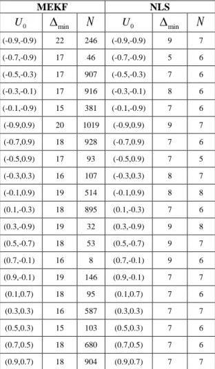
TABLEV.NECESSARY MINIMUM SHIFT FOR PARAMETER ( 2.55, 0.24) AND VARIOUS INITIAL
CONDITION SETS, 16 2 10 R Q I , 1010 MEKF NLS 0
U
minN
U
0
minN
(-0.9,-0.9) 22 246 (-0.9,-0.9) 9 7 (-0.7,-0.9) 17 46 (-0.7,-0.9) 5 6 (-0.5,-0.3) 17 907 (-0.5,-0.3) 7 6 (-0.3,-0.1) 17 916 (-0.3,-0.1) 8 6 (-0.1,-0.9) 15 381 (-0.1,-0.9) 7 6 (-0.9,0.9) 20 1019 (-0.9,0.9) 9 7 (-0.7,0.9) 18 928 (-0.7,0.9) 7 6 (-0.5,0.9) 17 93 (-0.5,0.9) 7 5 (-0.3,0.3) 16 107 (-0.3,0.3) 8 7 (-0.1,0.9) 19 514 (-0.1,0.9) 8 8 (0.1,-0.3) 18 895 (0.1,-0.3) 7 6 (0.3,-0.9) 19 32 (0.3,-0.9) 9 8 (0.5,-0.7) 18 53 (0.5,-0.7) 9 7 (0.7,-0.1) 16 8 (0.7,-0.1) 9 6 (0.9,-0.1) 19 146 (0.9,-0.1) 7 7 (0.1,0.7) 18 95 (0.1,0.7) 7 6 (0.3,0.3) 16 587 (0.3,0.3) 7 7 (0.5,0.3) 15 103 (0.5,0.3) 7 6 (0.7,0.5) 18 680 (0.7,0.5) 7 6 (0.9,0.7) 18 904 (0.9,0.7) 7 7In [7], we focused on the study of this particular parameter in the aim to avoid the oscillations of the EKF filter and to obtain the divergence of the method used. The EKF Matlab program already developed has been adapted to use the Gram Schmidt modified method. The Modified Extended Kalman Filter (MEKF) was therefore obtained.
Compared to the results obtained with EKF, the MEKF method improves the results in 60% of initial conditions. This means that MEKF diverges for a specific shift value, different for each initial condition, which is the threshold from which the parameter cannot be estimated. In other cases, the maximum iteration number is reached again.
Comparisons between MEKF and NLS simulations have also been done. The NLS method leads to the divergence of the algorithm for all initial conditions of the basin of the attractor and a necessary minimum shift is obtained, different in each case.
Table V shows a part of the results obtained for the parameter (-2.55,0.24) respectively using MEKF and NLS methods. Five initial condition sets are selected in four domains of
1,1
2. For each initial condition, the corresponding necessary minimum shiftmin
obtained and the iteration number N are given.
As seen in Table V, the parameter can be estimated until the minimum shift value and not beyond. For instance, for initial condition (-0.9, -0.9) , MEKF and NLS don’t estimated the parameter from min22 for MEKF and min 9 for
NLS. These minimum shift values are therefore necessary conditions corresponding to the method used. In all simulations, results show that higher minimum shift values are obtained with MEKF rather than NLS but the iteration number required by MEKF, and consequently, the time computing, are greater than that of NLS.
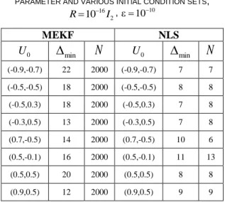
Regarding the EKF oscillations, this problem has been solved in more than half of the cases by using MEKF. But the NLS method is more efficient because it provides a necessary minimum shift for all the simulations done whereas MEKF does not work as shown in Table VI.
TABLEVI.NECESSARY MINIMUM SHIFT FOR PARAMETER AND VARIOUS INITIAL CONDITION SETS,
16 2 10 R I , 10 10 MEKF NLS 0
U
minN
U
0
minN
(-0.9,-0.7) 22 2000 (-0.9,-0.7) 7 7 (-0.5,-0.5) 18 2000 (-0.5,-0.5) 8 8 (-0.5,0.3) 18 2000 (-0.5,0.3) 7 8 (-0.3,0.5) 13 2000 (-0.3,0.5) 7 8 (0.7,-0.5) 14 2000 (0.7,-0.5) 10 6 (0.5,-0.1) 16 2000 (0.5,-0.1) 11 13 (0.5,0.5) 20 2000 (0.5,0.5) 8 8 (0.9,0.5) 12 2000 (0.9,0.5) 9 9Table VI shows some cases where the maximum iteration number is reached and the EKF filter still oscillates despite the use of MEKF. On the contrary, the NLS algorithm works until a necessary minimum shift, Dmin, from which it is not possible to estimate the map parameters.
The security of the time series used to estimate the chaotic map parameter is therefore guaranteed by taking the highest value of the necessary minimum shift obtained among all the simulations performed, i.e. 100 cases corresponding to 100 initial conditions of the basin of the considered attractor. Additional safety factor can also be applied to the value chosen.
7. Conclusion
These simulations have shown that both MEKF and NLS behavior depends on regular subsamplings of chaotic sequence terms considered. The two algorithms diverge for a particular subsampling corresponding to a necessary minimum shift, different for each parameter and each initial condition, from which it is not possible to estimate the parameter. The divergence of MEKF and NLS can be explained by round-off errors in the calculations, their accumulation and their propagation as the shift value is increased. Consequently, the estimated parameter precision decreases and finally, the algorithms diverge.
Moreover, this study carried out to test a single one-dimensional chaotic map to generate regular subsamplings shows that this particular case of M-p CPRNG is efficient in cryptography applications to choose cipher-keys. The security of a transmitted message is guaranteed by the shift value which must be chosen greater than the necessary minimum shift obtained. This shift value should be part of the secret key with the corresponding initial condition and parameter. Moreover, various initial condition, parameter and shift sets lead to the divergence of MEKF and NLS so that the secret key can be changed very often. Consequently, by using a such appropriate secret key and by changing it regularly, the cipher-key is immune against attack using the MEKF and NLS.
Finally, this study provides areas for future investigation on M-p CPRNG families.
10. References
[1] L. D. Cot, & C. Bès, “Study of the robustness of an enhanced CSK system by using the Extended Kalman Filter,” IEEE Conference publications, International Conference for Internet Technology and Secured Transactions (ICITST), Abu Dhabi, 202–207, (2011).
[2] M. A. Aziz-Alaoui, & C. Bertelle, From system
complexity to emergent properties (Understanding complex systems), Springer-Verlag, Berlin (2009).
[3] S. Hénaff, I. Taralova and R. Lozi, “Statistical and
spectral analysis of a newly weakly coupled maps system,” Indian J. Industr. Appl. Math., Vol. 2, 1– 17, (2009).
[4] S. Hénaff, I. Taralova and R. Lozi, “Exact and asymptotic synchronization of a new weakly coupled maps system,” J. Nonlin. Syst. Appl., Vol. 1, 87–95, (2010).
[5] R. Lozi, “New enhanced chaotic number
generators,” Indian J. Industr. Appl. Math., Vol. 1, 1–23, (2008).
[6] R. Lozi, “Emergence of randomness from chaos,”
Int. J. Bifurcation and Chaos, Vol. 22, No. 2,
1250021-1–1250021-15, (2012).
[7] L. D. Cot & R. Lozi, “Assessing the security of subsampling process using modified EKF and nonlinear least squares methods,” IEEE Conference
publications, International Conference for Internet
Technology and Secured Transactions (ICITST), London, 27–31, (2012).
[8] E. N. Lorenz, “Deterministic nonperiodic flow,” J.
Atmospheric Science, 20, 130-141, (1963).
[9] M. Hénon, “A Two-dimensional mapping with a
strange attractor,” Commun. Math. Phys., 50, 69-77, (1976).
[10] J. C. Sprott, Chaos and Time-Series Analysis,
Oxford University Press, Oxford, UK, (2003).
[11] M. S. Baptista, “Cryptography with chaos,” Phys.
Lett. A, 240, 50-54 (1998).
[12] M. R. K. Ariffin, & M. S. M. Noorani, “Modified
Baptista type chaotic cryptosystem via matrix secret key,” Phys. Lett. A, 372, 5427-5430 (2008).
[13] R. Lozi, & E. Cherrier, “Noise-resisting ciphering
based on a chaotic multi-stream pseudo-random number generator,” IEEE Conference publications, International Conference for Internet Technology and Secured Transactions (ICITST), Abu Dhabi, 91-96 (2011).
[14] R. Lozi & I. Taralova, “From chaos to ramdomness
via geometric undersampling,” to be published in
European Series in Applied and Industrial Mathematics (2013).
[15] M. S. Grewall, & A. P. Andrews, Kalman filtering
theory and practice using Matlab, 2nd Ed. Wiley &
Sons, New-York.
11. Acknowledgements
This work has been partially supported by the French National Research Agency (ANR) through the COSINUS program under the grant ANR-09-COSI-005 and by the PEPS INS2I 2012 program through the COIG project.