HAL Id: hal-01001685
https://hal.archives-ouvertes.fr/hal-01001685
Submitted on 4 Jun 2014
HAL is a multi-disciplinary open access archive for the deposit and dissemination of sci-entific research documents, whether they are pub-lished or not. The documents may come from teaching and research institutions in France or
L’archive ouverte pluridisciplinaire HAL, est destinée au dépôt et à la diffusion de documents scientifiques de niveau recherche, publiés ou non, émanant des établissements d’enseignement et de recherche français ou étrangers, des laboratoires
Estimation of spectral bounds in gradient algorithms
Luc Pronzato, Anatoly Zhigljavsky, Elena Bukina
To cite this version:
Luc Pronzato, Anatoly Zhigljavsky, Elena Bukina. Estimation of spectral bounds in gradient algo-rithms. Acta Applicandae Mathematicae, Springer Verlag, 2013, 127, pp.117-136. �10.1007/s10440-012-9794-z�. �hal-01001685�
Estimation of spectral bounds
in gradient algorithms
∗L. PRONZATO1,2, A. ZHIGLJAVSKY3 and E. BUKINA2 1 Author for correspondence
2 Laboratoire I3S, CNRS/Universit´e de Nice-Sophia Antipolis
Bˆat. Euclide, Les Algorithmes, 2000 route des lucioles, BP 121 06903 Sophia Antipolis cedex, France
3 School of Mathematics, Cardiff University
Senghennydd Road, Cardiff, CF24 4YH, UK [email protected]
[email protected] [email protected]
December 14, 2012
Abstract
We consider the solution of linear systems of equations Ax = b, with A a symmetric positive-definite matrix in Rn×n
, through Richardson-type iterations or, equivalently, the minimization of convex quadratic functions (1/2)(Ax, x) − (b, x) with a gradient algorithm. The use of step-sizes asymptotically distributed with the arcsine distribution on the spectrum of A then yields an asymptotic rate of convergence after k < n iterations, k → ∞, that coincides with that of the conjugate-gradient algorithm in the worst case. However, the spectral bounds m and M are generally unknown and thus need to be estimated to allow the construction of simple and cost-effective gradient algorithms with fast convergence. It is the purpose of this paper to analyse the properties of estimators of m and M based on moments of probability measures νk defined on the spectrum of A and generated by the algorithm
on its way towards the optimal solution. A precise analysis of the behavior of the rate of convergence of the algorithm is also given. Two situations are considered: (i) the sequence of step-sizes corresponds to i.i.d. random variables, (ii) they are generated through a dynamical system (fractional parts of the golden ratio) producing a low-discrepancy sequence. In the first case, properties of random walk can be used to prove the convergence of simple spectral bound estimators based on the first moment of νk. The second option requires a more careful
choice of spectral bounds estimators but is shown to produce much less fluctuations for the rate of convergence of the algorithm.
keywords estimation of leading eigenvalues; arcsine distribution; gradient algorithms; con-jugate gradient; Fibonacci numbers
MSC 65F10; 65F15
∗
Part of this work was accomplished while the first two authors were invited at the Isaac Newton Institute for Mathematical Sciences, Cambridge, UK; the support of the INI and of CNRS is gratefully acknowledged. The work of E. Bukina was partially supported by the EU through a Marie-Curie Fellowship (EST-SIGNAL program: http://est-signal.i3s.unice.fr) under the contract Nb. MEST-CT-2005-021175.
1
Introduction and motivation
For {νk}∞k=0a sequence of probability measures supported on a real interval [m, M ], the sequence
of first moments µ(k)1 =RmMt νk(dt) gives obvious estimators of m and M through
b mk= min j=0,...,kµ (j) 1 and cMk= max j=0,...,kµ (j) 1 . (1)
We consider the behavior of estimators (1) and their extensions defined below when νk are
prob-ability measures associated with a gradient algorithm for the minimization of a convex quadratic function with matrix A ∈ Rn×n (symmetric positive-definite) and µ(k)1 = (Agk, gk)/(gk, gk), with
gk, the gradient at step k, obeying the recurrence equations
gk+1= gk− γkAgk, k = 0, 1, 2 . . . (2)
Here, γk > 0 is the step-size at iteration k and is determined by some rule that
charac-terizes the algorithm. For instance, γk = 1/µ(k)1 for the Steepest Descent (SD) algorithm,
γk = (Agk, gk)/(A2gk, gk) for the method of Minimum Residues (MR), see [8], [18, p. 134],
and γk = 1/µ(k−1)1 for the method of Barzilai and Borwein [1]. The algorithms considered in
[3, 12, 20] rely on the generation of an infinite sequence of step-sizes γk(possibly random), such
that βk = 1/γk ∈ [m, M] for all k, with m and M respectively the minimum and maximum
eigenvalues of A. As shown in [16], when the sequence {βk} is asymptotically distributed with
the arcsine density in [m, M ], then the asymptotic rate of convergence is competitive compared to that of Conjugate Gradients (CG) [7], Conjugate Residuals (CR) [5, p.547], or other methods based on Krylov spaces, like e.g. MINRES [11] (it coincides with that exhibited by CG and CR in the worst case, in terms of choice of the starting point and locations of the n − 2 internal eigenvalues of A in (m, M ), when the algorithm is stopped before n iterations). Such algorithms, with step-sizes generated externally, are simpler than CR and CG and thus of particular interest in situations where n is so large that the algorithm is stopped well before n iterations (in partic-ular, it is shown in [22] that for some sequences of step-sizes the number of scalar products to be computed out of k iterations only grows as O(log k), see also Sect. 3.3 and 5). The generation of suitable sequences of step-sizes γk requires, however, the knowledge of the spectral bounds m
and M . Since they are usually unknown, it is suggested in [22, 16] to estimate them through the evaluation of moments of probability measures generated by the algorithm itself. It is the purpose of this paper to analyse the asymptotic properties of the estimators (1) of the leading eigenvalues of A. In particular, two situations will be considered: (i) the γk form a sequence of
i.i.d. random variables, (ii) they are constructed from a low discrepancy sequence. In addition, a more precise analysis of the behavior of the rate of convergence of the algorithm than in [22, 16] will be provided (Sect. 4).
2
A sequence of probability measures associated with a gradient
algorithm
Consider a linear system of equations
Ax = b , (3)
where x ∈ Rn is an unknown vector, A is a n × n symmetric positive-definite matrix such
Equivalently, one may consider the minimization of the convex quadratic function
f (x) = 1
2(Ax, x) − (b, x) . (4)
The gradient gk = Axk− b then corresponds to the (minus) residual of the system (3) at xk.
Richardson-like methods for solving (3) correspond to gradient algorithms for minimizing (4) and obey to the following iterations
xk+1= xk− γkgk, k = 0, 1, 2 . . . , (5)
where x0 ∈ Rn is a starting vector and γk > 0 is the step-size at iteration k. The methods to
be considered are of particular interest in situations where the dimension n can be very large (it could even be infinite, with A a self-adjoint operator in a Hilbert space, but we shall restrict the presentation to the finite dimensional situation) and we shall assume that n is much larger than the number of iterations k∗ needed to achieve the precision required (formally, k∗ = o(n) with k∗→ ∞ in asymptotic considerations).
The iterations (5) can be rewritten in terms of gradients gk, which gives (2), with g0 =
Ax0 − b ∈ Rn the initial gradient. We define the rate of convergence of the algorithm (5)
towards the solution at iteration j as
rj =
(gj+1, gj+1)
(gj, gj)
;
the rate of convergence after k iterations is then
Rk= k−1Y j=0 rj = (gk, gk) (g0, g0) . (6)
Other convergence rates, which are asymptotically equivalent to rj (see [14, Th. 6]), can also
considered. In particular,
rj′ = f (xj+1) − f(x∗) f (xj) − f(x∗)
= (A−1gj+1, gj+1) (A−1gj, gj)
is often used when minimizing a quadratic function (4), with x∗ = A−1b its minimizer.
The method of Steepest-Descent (SD) chooses γkin (5) that minimizes rk′ and the method of
Minimum Residues (MR) chooses γkthat minimizes rk, both are myopic and only look one-step
forward. The method of Conjugate Gradients (CG) minimizes
R′k= k−1Y j=0 r′j = f (xk) − f(x ∗) f (x0) − f(x∗) = (A −1g k, gk) (A−1g0, g0)
with respect to the sequence γ0, γ1, . . . , γk−1 and the method of Conjugate Residuals (CR) does
the same with Rk; we shall denote RCRk = minγ0,...,γk−1Rk. Although CR minimizes Rk for all
k, for any k < n one may nevertheless have, in the worst case with respect to the starting point x0 and eigenvalues λ2, . . . , λn−1, RCRk = R∗k, where
R∗k= Ã Rk/2∞ + R−k/2∞ 2 !−2 = Ck−2 µ ρ + 1 ρ − 1 ¶ ,
with ρ = M/m the condition number of A, Ck(·) the k-th Chebyshev polynomial of the first
kind, Ck(t) = cos[k arccos(t)] = (1/2)[(t +√t2− 1)k+ (t −√t2− 1)k], and
R∞= lim k→∞(R ∗ k)1/k = µ√ ρ − 1 √ρ + 1 ¶2 , (7)
see [4, 15]. Hence, although one regularly observes values of RCRk that are significantly smaller than R∗
k for k < n (and although RnCR= 0, that is, the solution is found exactly in n iterations
in the exact arithmetic), for any k < n one has maxx0,ARCRk = R∗k, with (Rk∗)1/k decreasing
monotonically to R∞as k → ∞. As shown in [16], the same asymptotic rate R∞can be obtained when the sequence {βk} = {1/γk} is generated externally with some suitable distribution in
[m, M ]; see also Sect. 4.
From (2), the gradient gk after k iterations can be written as
gk= Pk(A)g0, (8)
where Pk denotes the polynomial Pk(A) = (I − γk−1A)(I − γk−2A) . . . (I − γ0A) .
Let m = λ1 ≤ . . . ≤ λn = M be the eigenvalues of A and {q1, . . . , qn} be the set of
corresponding orthonormal eigenvectors (we assume that no information is available about the eigenvalues λi and eigenvectors qi, i = 1, . . . , n, and that the condition number M/m may be
large). When decomposing the initial vector g0 in the basis {q1, . . . , qn} as g0 =Pni=1αiqi, (8)
implies gk = n X i=1 αiPk(λi)qi (9)
for all k ≥ 1. The squared L2-norm of g0 is kg0k2= (g0, g0) =Pni=1α2i and the squared L2-norm
of gk is thus kgkk2 = (gk, gk) = Pni=1α2iPk2(λi) . The convergence rate (6) after k iterations is
then given by Rk= n P i=1 α2 iPk2(λi) n P i=1 α2 i = n X i=1 p(0)i Pk2(λi) , where p(0)i = α2 i ± Pn j=1 α2 j ≥ 0 and Pn i=1p (0) i = 1.
Without loss of generality all α2
i can be assumed to be strictly positive. Indeed, if αi= 0 for
some i then the matrix A = Pnj=1λjqjq⊤j can be replaced with ˜A =Pj6=iλjqjqj⊤; the equality
αi = 0 would mean that (A x0, qi) = (b, qi) (and therefore (A xk, qi) = (b, qi) for all k).
From (9), (gk, qi) = αiPk(λi). We define p(k)i = (gk, qi) 2 (gk, gk) = α 2 iPk2(λi) Pn j=1α2jPk2(λj)
and interpret this as a mass at λi. Then, the measure νk defined by its masses νk(λi) = p(k)i at
λ = λi (i = 1, . . . , n) characterizes the normalized vector gk/kgkk (up to the signs of the (gk, qi),
which are irrelevant for analyzing the behavior of the algorithm). For any real α, define µ(k)α as
the α-th moment of the probability measure νk:
µ(k)α = µα(νk) = n X i=1 λαip(k)i = (A αg k, gk) (gk, gk) . (10)
Using the basic iteration (2), we obtain the following updating formula which expresses the measure νk+1 through the measure νk:
p(k+1)i = νk+1(λi) = αi2Pk+12 (λi) (gk+1, gk+1) = α 2 i(1 − γkλi)2Pk2(λi) (gk+1, gk+1) = (1 − γkλi) 2p(k) i rk , i = 1, . . . , n , (11) where k ≥ 0 and rk= (gk+1, gk+1) (gk, gk) = (gk, gk) − 2γk(Agk, gk) + γ 2 k(A2gk, gk) (gk, gk) = 1 − 2γk µ(k)1 + γk2µ(k)2 . (12)
3
Estimation of the leading eigenvalues of A
3.1 Defining the estimators
Take any probability measure ν on [m, M ] with 0 < m < M < ∞ and denote by µα its moment
of order α, µα= µα(ν) =RmMtαν(dt) (so that µα(νk) is defined by (10)). The Cauchy-Schwarz
inequality implies µα+2µα ≥ (µα+1)2 for any α . Moreover, t(M − t) ≥ 0 for all t ∈ [m, M] so
that RmMtα(M − t) ν(dt) = Mµ
α− µα+1 ≥ 0; that is, µα+1/µα ≤ M. Similarly, m ≤ µα+1/µα.
We thus obtain the following chain of inequalities
m ≤ µ(k)1 ≤ µ(k)2 µ(k)1 ≤ µ(k)3 µ(k)2 ≤ µ(k)4 µ(k)3 ≤ · · · ≤ M , (13)
which are valid for all k = 0, 1, . . . ; note that µ(k)0 = 1 for all k.
In what follows we shall restrict our attention to the estimators of m and M defined by b mk= min j=0,...,kµ (j) 1 , cM (i) k = maxj=0,...,kµ (j) i /µ (j) i−1, i ≥ 1 . (14)
According to (13), the larger i in cMk(i)the more precise the estimation of M , which has a signif-icant influence on the behavior of the algorithm, see [22]. Calculating high order moments has some computational cost, however, and a compromise must be made. The algorithm presented in Sect. 5 uses i = 4.
Let {αk} denote a sequence in [−1, 1] with asymptotic distribution function Fα(·) symmetric
with respect to zero (different types of sequences will be considered below). We shall consider algorithms defined as follows: we initiate (5) by two SD iterations with γk= 1/µ(k)1 , or two MR
iterations with γk = µ(k)1 /µ (k)
2 ; for each subsequent iteration the inverse step-size βk = 1/γk is
obtained by rescaling the k-th element αk of the sequence {αk} into [ bmk, cMk], that is,
βk= αk( cMk− bmk)/2 + ( cMk+ bmk)/2 . (15)
The assumption that the βk are generated by symmetric pairs in [m, M ], that is, β2j+1 =
M + m − β2j, is used in [16] to derive the expression for the asymptotic convergence rate R of
the algorithm, R = limk→∞R1/kk ; see also Sect. 4. This is why we shall also consider the case when (15) is replaced by
(
β2j = αj( cM2j− bm2j)/2 + ( cM2j+ bm2j)/2 ,
β2j+1 = −αj( cM2j+1− bm2j+1)/2 + ( cM2j+1+ bm2j+1)/2 .
As shown in [22], using the largest β first in a pair (β2j, β2j+1) permits to improve the
mono-tonicity of the algorithm (5). We shall thus also consider the case when (
β2j = |αj|( cM2j − bm2j)/2 + ( cM2j+ bm2j)/2 ,
β2j+1 = −|αj|( cM2j+1− bm2j+1)/2 + ( cM2j+1+ bm2j+1)/2 ,
(17)
Lemma 1 below shows that ( bmk+ cMk)/2 converges to (m+M )/2 so that the symmetry condition
with respect to (m + M )/2 will be asymptotically satisfied.
3.2 Consistency of mbk and cMk
The estimators bmk and cMk satisfy the following asymptotic symmetry property.
Lemma 1 Assume that in algorithm (5) βk = 1/γk is generated according to one of the rules
(15), (16) or (17), with bmk and cMk = cMk(i) given by (14) for all k for some i ≥ 1 and {αk}
having an asymptotic distribution function Fα(·) in [−1, 1] symmetric with respect to zero. Then
we have
M − M∞= m∞− m ≥ 0 , (18)
where m∞= limk→∞mbk and M∞= limk→∞Mck.
The proof, based on establishing a contradiction if we assume that the symmetry condition (18) is violated, is given in Sect. 6.
To obtain a more precise characterization of the limiting behaviors of bmk and cMk we shall
make use of the following property, shown in [16].
Theorem 1 Set βk = 1/γk (k = 0, 1, . . .) and assume that βk > 0 and βk ∈ {m, M} for all k/
and that the sequence {βk} has an asymptotic distribution function Fβ(·) which is supported on
an interval [m′, M′] with 0 < m′ ≤ M′ < ∞. Suppose, moreover, that this limiting distribution
satisfies Z log(t − λ)2dFβ(t) < max ½Z log(M − t)2dFβ(t) , Z log(t − m)2dFβ(t) ¾ , (19)
for all λ ∈ (m, M). Then the algorithm (5) associated with the sequence {βk} is such that
lim
k→∞νk(λi) = 0 for all i = 2, . . . , n − 1. Furthermore, there exist constants C > 0, k0 > 0 and
0 ≤ θ < 1 such that Pn−1i=2 νk(λi) ≤ Cθk for k > k0.
The main condition in Th. 1 is (19); it implies that the ratio P2
k(λ)/(Pk2(m) + Pk2(M )) tends
to 0 (as k → ∞) exponentially fast for any λ ∈ (m, M). It means that once the attraction of the sequence {νk} to the set of measures supported at m and M is obtained, i.e. νk(m)+νk(M ) → 1,
it is roughly enough to consider the behavior obtained for two-point measures.
Remark 1 The attraction of the sequence {νk} to the set of measures supported at m and M
does not imply that bmk → m and cMk → M. Indeed, consider the case when the sequence of
step-sizes is self-generated by the algorithm itself. For instance, for SD we have βk = µ(k)1 for
all k and the limiting measure for {βk} is the two-point measure allocating weights 1/2 at z and
M + m − z for some z ∈ (m, M). The condition (19) is then equivalent to z belonging to the stability interval defined in [13, 14], see [16], and m∞ and M∞ satisfy (18) but do not coincide with m and M .
Remark 2 When the βk are generated by (16) or (17), then, under the conditions of Lemma 1,
they asymptotically satisfy β2j+1 = M + m − β2j. When ν2j is a two-point measure supported
at m and M , we then have ν2j+2 = ν2j. Additionally to Th. 1, p(2j)1 tends to a constant p∞ as
j → ∞, with p∞ depending on the starting measure ν0 ( i.e., on the starting point x0) and on
the spectrum of A.
We first consider the case when the αk used to generate the step-sizes γk = 1/βk via (15)
are i.i.d. with a suitable distribution.
Theorem 2 Assume that in algorithm (5) βk = 1/γk satisfies (15) with bmk and cMk = cMk(i)
given by (14) for all k for some i ≥ 1 and that the αk are i.i.d. in [−1, 1] with a distribution
function Fα(·) symmetric with respect to zero. Assume, moreover, that
Z
log(t − u)2dFα(t) <
Z
log(1 − t)2dFα(t) < ∞ for all u ∈ (−1, 1) (20)
and that Fα(1 − x) < 1 for any x > 0. Then, m∞= limk→∞mbk= m and M∞= limk→∞Mck =
M almost surely.
The proof is given in Section 6. The idea is roughly as follows. In view of Th. 1, the asymptotic behavior of the measures νk is very similar to the behavior of measures ˜νkwhich use
the same updating formulas but are supported on the two-point set {m, M}. However, for this sequence of two-point measures ˜νk the sequence of random variables log ˜νk(m) − log(1 − ˜νk(m))
is a random walk and therefore the values ˜νk(m) approach 0 and 1 (with any fixed precision)
infinitely often. This implies that the sequence of first moments of ˜νkgets arbitrarily close to m
and M infinitely often. The same occurs for the original sequence of measures νk (proving this
requires some technicalities).
As shown in the next theorem, when using cMk= cMk(i) with i ≥ 2 we do not have to use i.i.d.
αk to obtain m∞= m and M∞= M . Moreover, the sequence {βk} can be generated by (16) or
(17).
Theorem 3 Assume that in algorithm (5) the βk = 1/γk are generated according to one of the
rules (15), (16) or (17), with {αk} having an asymptotic distribution function Fα(·) in [−1, 1]
symmetric with respect to zero, and that bmk and cMk= cMk(i) are given by (14) for all k for some
i ≥ 2. Assume, moreover, that Fα(·) satisfies (20) and that Fα(1 − x) < 1 for any x > 0. Then,
m∞= limk→∞mbk= m and M∞= limk→∞Mck= M .
The proof is given in Section 6. The proof of Th. 2 must be modified since, when the αi
are not randomly generated, we cannot be sure to have simultaneously a large value of βk and
a small value of µ(k)1 , see part (ii) of the proof of Th. 2. As a consequence, i = 1 does not guarantee the convergence of bmk and cMk= cMk(i) to respectively m and M and we now have to
use a more precise estimator of M with i > 1.
When the αk are i.i.d., the result of Th. 3 holds almost surely. The theorem also
cov-ers the case where {αk} is a deterministic sequence, for instance generated via a
dynami-cal system, which permits to obtain sequences of rates rk much less erratic than when
us-ing random step-sizes, see Sect. 4. Notice that the proof of Th. 3 does not apply when c
Mk = cMk(1) = maxj=0,...,kµ(j)1 (although simulations seem to indicate consistency of bmk and
c
3.3 Controlling the number of updates for mbk and cMk
The calculations of µ(k)1 and µ(k)2 /µ(k)1 require the evaluation of several inner products in Rn; therefore, by minimizing the number of iterations where bmk or cMk are updated we can reduce
the computational cost of the algorithm. Updates of bmk and cMk in the situation of Th. 2 or
Th. 3 can be stimulated by the convergence of the measure νk to the set of measures supported
at m and M and by the fact that, on the route to this set of two-point measures, νkcan fluctuate
between measures supported at m (when bmk+ cMk > m + M ) and measures supported at M
(when bmk+ cMk < m + M ). On the other hand, iterations where bmk (resp. cMk) has a good
chance to get significantly updated are those for which the next measure νk+1 will be close to
the delta measure at m (resp. at M ). This may happen in particular when βk is the smallest
(resp. largest) among all βj, j ≤ k. It can be related to record moments for the αj and we
shall thus consider the situation where updates of bmk or cMk are allowed only at those iterations
where αj is a new record.
For any sequence {zk} = z0, z1, z2. . . define the two sequences or record moments {Lminj } =
{Lmin
j }[{zk}] and {Lmaxj } = {Lmaxj }[{zk}] by Lmin0 = Lmax0 = 0 and, for all j ≥ 0,
Lminj+1= min{k > Lminj : zk< zLmin j } , L
max
j+1 = min{k > Lmaxj : zk> zLmax j } .
We also define the numbers of lower and upper record moments, respectively δmin
j = δjmin[{zk}]
and δjmax= δjmax[{zk}], by
δjmin = #{i ≥ 0 : Lmini ≤ j} = 1 + max{i ≥ 0 : Lmini ≤ j} , δmaxj = #{i ≥ 0 : Lmaxi ≤ j} = 1 + max{i ≥ 0 : Lmaxi ≤ j} .
For any k, denote by ¯βk the value obtained when m and M are substituted for bmk and cMk in
(15), (16) or (17). The record moments for { ¯βk} then coincide with those for {αj}, but those for
βk may differ since in general bmk+ cMk6= m + M. However, due to Lemma 1, the dissimilarity is
asymptotically negligible. When (15) is used, upper (resp. lower) record moments for ¯βkcoincide
with upper (resp. lower) record moments for αk; when (16) or (17) is used, records for ¯βkarrive
in pairs, records for ¯β2j and ¯β2j+1 being associated with a αj that becomes new record (either
lower or upper).
3.3.1 {αk} forms an i.i.d. sequence of random variables
When the αkare i.i.d., the numbers of lower and upper record moments δminj [{αk}] and δmaxj [{αk}]
satisfy δmin
j / log j → 1 and δjmax/ log j → 1 almost surely, see [2, p. 258]. Therefore, when we
use (15), δminj [{ ¯βk}]/ log j → 1 and δmaxj [{ ¯βk}]/ log j → 1, whereas δjmin[{ ¯βk}]/ log j → 2 and
δjmax[{ ¯βk}]/ log j → 2 when we use (16) or (17).
3.3.2 {αk} is constructed from a low discrepancy sequence
Consider in particular the sequence given by αk = cos(πuk) for all k ≥ 0, with uk = (k + 1)ϕ
mod 1 (the fractional part of (k + 1)ϕ), where ϕ = (√5 + 1)/2 ≃ 1.61803 . . . is the golden ratio (note that the sequence {uk} can equivalently be constructed through the dynamical system
u0 = ϕ−1, uk+1 = (uk+ϕ) mod 1, k ≥ 0). This construction is motivated by the associated rate
of convergence of the algorithm, see Sect. 4. The corresponding sequences of record moments are {Lminj }[{αk}] = {0, 1, 4, 12, 33, . . .} and {Lmaxj }[{αk}] = {0, 2, 7, 20, 54, . . .}. Denote {FN}∞N =1=
{1, 1, 2, 3, 5, 8, 13, 21, 34 . . .} the sequence of Fibonacci numbers, with exact expression FN =
(ϕN − (−1/ϕ)N)/√5. {Lminj } and {Lmaxj } can then be expressed in terms of the Fibonacci numbers Fj as follows: Lminj = F2j+1− 1, Lmaxj = F2j+2− 1 for j = 0, 1, . . . This directly follows
from the following two classical results of the theory of Diophantine approximations: (i) for the sequence {kζ mod 1}, with any irrational ζ, the successive minimal and maximal values occur when k = q in the denominator of a convergent p/q for ζ in the standard continued fraction expansion of ζ, see [19]; (ii) the convergents of ζ = ϕ − 1 are Fj/Fj+1 for j > 1. The number of
upper record moments for {αj} is then δkmax[{αj}] = 1 + max{j : F2j+2− 1 ≤ k} = 1 + max{j :
F2j+2 ≤ k + 1}. Similar to Proposition 7 in [22] we can show that for all k > 1 we have the
inequalities C0log k − 1 < δk < C0log k + 1 with C0 = 1/[2 log(ϕ)] ≃ 1.039. This yields the
asymptotic relation δk = C0log k + O(1) as k → ∞.
When we use (15), the sequence of record moments for { ¯βk} is the same as for {αk}. If we
use (17), then the sequences of record moments for ¯βk are {Lminj }[{ ¯βk}] = {0, 1, 3, 5, 9, 15, . . .}
and {Lmax
j }[{ ¯βk}] = {0, 2, 4, 8, 14, . . .}, with Lminj+1 = Lmaxj + 1 for j = 0, 1, . . . and, in terms of
Fibonacci numbers, Lmaxj = 2(Fj+2−1) for j = 0, 1, . . . The number δkof upper record moments
for { ¯βj} thus satisfies δk/ log k → 2C0 = 1/ log(ϕ) ≃ 2.078 as k → ∞; the same is obviously
true for the number of lower record moments. If we use (16), the sequences of record moments for ¯βk are {Lminj }[{ ¯βk}] = {0, 3, 4, 9, 14, 25 . . .} and {Lmaxj }[{ ¯βk}] = {0, 1, 2, 5, 8, 15, 24, . . .}; that
is, in terms of Fibonacci numbers, Lmaxj = 2(Fj+1− 1) if j is even and Lmaxj = 2Fj+1− 1 if j is
odd, Lmin
j = 2(Fj+2− 1) if j is even and Lmaxj = 2Fj+2− 1 if j is odd. The numbers of upper
and lower record moments satisfy again δk/ log k → 1/ log(ϕ) ≃ 2.078 as k → ∞.
Example 1 We set n = 800, m = 1 and M = 1000, the eigenvalues of A are uniformly distributed in [m, M ] and b = Ac in (3, 4) with c uniformly distributed on the unit n-dimensional sphere Sn. We apply the gradient iterations (5) with x0 uniformly distributed on Sn; the first
two iterations correspond to the method of minimum residues with γk= µ(k)1 /µ(k)2 , k = 0, 1, and
the subsequent iterations use {γk} = {1/βk}, where the βk are generated via (17) using the low
discrepancy sequence {αk} above: αk = cos(π[(k + 1)ϕ mod 1]) for all k ≥ 0. We compare the
behaviors of two estimators of m and M . The first one corresponds to bmk and cMk(4) given by
(14), the second to e m2j+1 = min j∈Lα µ(2j+1)1 and fM2j+2 = max j∈Lα µ(2j+2)4 µ(2j+2)3 , (21) where Lα = {Lminj }[{αk}]S{Lmaxj }[{αk}] denotes the sequence of lower and upper record
mo-ments for {αk}. This construction is motivated by the fact that when αj becomes a new (lower
or upper) record, then β2j+1 is large and µ(2j+1)1 has a good chance to be small, while β2j+2 is
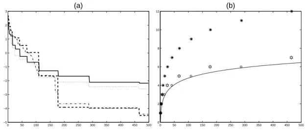
small and µ(2j+2)4 /µ(2j+2)3 has a good chance to be large. The precision of the estimation of m and M given by the two estimators is compared in Fig. 1a. Figure 1b indicates the number of record moments for {αk} together with the number of iterations where emkand fMk are updated.
One may notice that both em2j+1 and fM2j+2 are updated each time αj is a new record.
4
Fluctuations of the sequence of convergence rates
When νk is a two-point measure supported at m and M , applying two successive iterations (11)
0 50 100 150 200 250 300 350 400 450 500 −5 −4 −3 −2 −1 0 1 2 3 (a) 0 50 100 150 200 250 300 350 400 450 500 0 2 4 6 8 10 12 (b)
Figure 1: (a) Evolution of log10(M − cMk) and log10( bmk− m) with bmk and cMk = cMk(4) given
by (14), respectively in dotted and dash-dotted lines, and evolution of log10(M − fMk) and
log10( emk − m) with emk and fMk given by (21), respectively in solid and dashes lines. (b)
Number of record moments δkmax[{αj}] (hexagrams) and δkmin[{αj}] (circles) as functions of k,
the number of iterations where emk and fMk are updated are indicated respectively by stars and
dots, the solid line corresponds to (log k)/[2 log(ϕ)] ≃ 1.039 log k.
the particular measure νk, rkrk+1= R22(βk), where
R2(β) = (M − β)(β − m) β(M + m − β) . This is the key-point used in [16] to prove the following.
Theorem 4 Assume that the conditions of Th. 1 are satisfied and that, moreover, the βk are
generated by symmetric pairs for large k; that is, β2j+1 = M + m − β2j for all j ≥ j0, with
β2j ∈ [m + ε, M − ε] for some ε ∈ (0, (M − m)/2). Then,
lim k→∞ 1 klog Rk= Z log ¯ ¯ ¯ ¯(M − t) (t − m)t (m + M − t) ¯ ¯ ¯ ¯ dFβ(t) = Z log(t − m) 2 t2 dFβ(t) , (22) where Rk is defined by (6).
Th. 4 applies in particular when Fβ(·) has the arcsine density fǫ(·) on [m + ǫ, M − ǫ],
fǫ(β) =
1
πp(β − m − ǫ)(M − ǫ − β), with ǫ < (M − m)/2. In that case, as k → ∞,
R1/kk → Rarcsine,ǫ = exp ½Z M −ǫ m+ǫ log(β − m) 2 β2 fǫ(β) dβ ¾ = Ã M − m + 2pǫ(M − m − ǫ) M + m + 2p(M − ǫ)(m + ǫ) !2 (23) = R∞(1 + 4pǫ(M − m)) + O(ǫ) , ǫ → 0 ,
with R∞ given by (7), see [16]. In the rest of the section we are interested in the extension of Th. 4 to the case where the βk are generated by (16) or (17) with estimated bmk and cMk and to
the fluctuations of Rk1/k along its way to its limiting value.
The fact that in (16, 17) bmk and cMk are estimated brings a slight difference with Th. 4 in
terms of asymptotic rate of convergence. This difference is marginal, however, as shown in the next theorem.
Theorem 5 Assume that in algorithm (5) the βk are generated by pairs as in (16) or (17), with
b
mk and cMk= cMk(i) given by (14) for all k for some i ≥ 2, and that the αj have an asymptotic
distribution function Fα(·) in [−1 + δ, 1 − δ], 0 < δ < 1/2, symmetric with respect to zero and
satisfying (20) and Fα(1 − δ − x) < 1 for any x > 0. Then the result (22) of Th. 4 remains
valid, with Fβ(·) a rescaled version of Fα(·) in some interval [m + ǫ′, M − ǫ′], that is,
dFβ(t) = 2 M − m − 2ǫ′ dFα µ 2t − m − M M − m − 2ǫ′ ¶ , (24) where ǫ′ satisfies δ(M − m)/2 ≤ ǫ′ ≤√M (√M +√m)δ/2 + O(δ2) . (25)
The proof is given in Sect. 6. The fact that the αknow lie in [−1 + δ, 1 − δ] with δ > 0 makes
it necessary to slightly modify the proof of Th. 3.
Consider now the fluctuations of the asymptotic convergence rate around its limiting value. Suppose that m and M are perfectly estimated, so that β2j+1 = M + m − β2j in (16, 17), with
the β2j having a distribution Fβ(·) satisfying the condition in Th. 4. Since the βk are exactly
symmetric in [m, M ], we can take δ1 = 0 in the proof of Th. 5, so that
log[R2(β2j)] − Bθ2j < 1
2 log(r2jr2j+1) < log[R2(β2j)] + Bθ
2j
for some B > 0 and j > j1 large enough, which gives
¯ ¯ ¯ ¯ ¯ ¯ 1 2 log µ R2i R2j1 ¶ − i−1 X j=j1 log[R2(β2j)] ¯ ¯ ¯ ¯ ¯ ¯< ∞ X j=0 Bθ2j = B 1 − θ, with θ as in Th. 1. Define Lα = Z log[R2(t)] dFβ(t) = Z log à 1 + t t +M +mM −m !2 dFα(t) , Vα = Z log à 1 + t t + M +mM −m !2 − Lα 2 dFα(t) .
(Note that both quantities are well defined when Fα(·) is concentrated on [−1 + δ, 1 − δ], δ > 0.)
When the αk are i.i.d. with the distribution Fα(·), we have, for i → ∞,
1 i log p R2ia.s.→ Lα, √ i µ log√R2i i − Lα ¶ d → ξ ∼ N (0, Vα) ,
and
R1/2i2i a.s.→ exp(Lα) ,
√
i³R2i1/2i− exp(Lα)
´ d
→ ξ ∼ N (0, Vαexp(2Lα)) .
Moreover, from the law of the iterated logarithm,
lim sup
i→∞
log√R2i− iLα
√
2iVα√log log i
= 1 a.s. and lim inf
i→∞
log√R2i− iLα
√
2iVα√log log i = −1 a.s. ,
implying that, for any ε > 0,
R1/2i2i > exp · Lα+(1 − ε) √ 2Vαlog log i √ i ¸ (26)
infinitely often (a.s.), and thus indicating that the fluctuations of the normalized convergence rate R1/2i2i are unavoidably large.
Suppose now that {αk} is constructed from a low-discrepancy sequence, as in Sect. 3.3. Then
¯ ¯ ¯ ¯ ¯ ¯ 1 i − j1 i−1 X j=j1 log[R2(β2j)] − Lα ¯ ¯ ¯ ¯ ¯ ¯< Cα log i i
for some large enough j1 (see the proof of Th. 5) and some constant Cα depending on the
sequence considered, see, e.g., [10]. Therefore, in that case the normalized convergence rate satisfies R1/2i2i / exp(Lα) < iCα/i and shows much less fluctuations on its route to its limiting
value exp(Lα) than when the αkare i.i.d. random variables. Indeed, denoting D2ithe difference
R2i1/2i− exp(Lα), we have
(D2i)i.i.d. |(D2i)LDS| > exph(1−ε) √ 2V√αlog log i i i − 1
iCα/i− 1 i.o. a.s. for any ε > 0
where the right-hand side behaves like c√i log log i/ log i as i → ∞ (c = (1 − ε)√2Vα/Cα).
This justifies the preference given to low discrepancy sequences over random sequences in the algorithms presented in [22]. One of them is summarized in Sect. 5.
Example 2 We consider the same problem as in Sect. 3.3 (we take now x0 = (105, 1, 1, . . . , 1)⊤
to slow down convergence and better illustrate the different behaviors for the two types of step-size sequences). The βk are generated by (17) with bmk and cMk= cMk(4) given by (14). Figure 2
shows R1/2i2i as a function of i for the cases when {αk} is the low discrepancy sequence given by
αk = cos(π[(k + 1)ϕ mod 1]) for all k ≥ 0 and when {αk} is a sequence of i.i.d. random variables
having the arcsine distribution; both sequences are generated on [−1 + δ; 1 − δ] with δ = 0.005.
5
Prototype algorithm and simulation results
The estimation of the spectral bounds m and M via (21) permits to construct a gradient al-gorithm which is quite parsimonious in terms of number of computations of inner products. In order to avoid using multiplications by A when calculating µ(k)1 and µ(k)4 /µ(k)3 , the following recursions are used:
µ(k)1 = (Agk, gk) (gk, gk) = βk · 1 −(g(gk, gk+1) k, gk) ¸
50 100 150 200 250 300 350 400 450 500 0.96 0.965 0.97 0.975 0.98 0.985 0.99 0.995 i R 1 /2 i 2 i
Figure 2: Rate R1/2i2i as a function of i for αk= cos(π[(k + 1)ϕ mod 1]) for all k ≥ 0 (solid line)
and for {αk} a random i.i.d. sequence having the arcsine distribution (dash-dotted line). The
dashed line indicates the bound Rarcsine,ǫ′ given by (23) with ǫ′ = δ(M − m)/2 (δ = 5 · 10−3), see
(25); the dotted line denotes the right-hand side of (26).
and µ(k−1)4 µ(k−1)3 = (A2gk−1, A2gk−1) (A2g k−1, Agk−1) = βk−1+ βk (βk(gk+1− gk) + βk−1(gk−1− gk), gk+1− gk) (βk(gk+1− gk) + βk−1(gk−1− gk), gk−1− gk) ,
which can easily be derived from (2). We generate the βk= 1/γkaccording to (17) using the low
discrepancy sequence αk= cos(π[(k + 1)ϕ mod 1]) for all k ≥ 0. The construction (17) tends to
favor the estimation of m against that of M , see [22], which results in the concentration of νk
at M . From (12), the convergence is monotonic at step k (i.e., rk< 1) when βk > µ(k)2 /(2µ (k) 1 ).
When νk gets close to the delta measure at M , this ratio becomes close to M/2 when M/m
is large, and the monotonicity condition is violated frequently (approximately every second iteration). In the algorithm proposed below this is avoided by forcing νkto become concentrated
at m rather than M , the monotonicity property rk< 1 being always satisfied when µ(k)2 /(2µ (k) 1 )
is close to m/2 since βkis larger than bmk > m. This can be achieved by using a step with large βk
when νk−1 becomes close to the delta measure at M . In practice, we simply use βk= cMk when
we observe cMk > cMk−1. The algorithm is summarized below; its MATLAB implementation
is available at http://www.i3s.unice.fr/~pronzato/Matlab/goldenArcsineQ.m. We define vj = ϕ(j + 1) mod 1 and, for j = 0, 1, . . . we set
zj= (1+cos(πuj))/2, where u2j= min{vj, 1−vj}, u2j+1= max{vj, 1−vj} .
Algorithm
Stage I (initialization)
I.1 Choose x0 and compute g0= Ax0− b.
I.2 Choose ǫ > 0 used in the stopping rule.
I.3 Set Lmax= {2Fi+2− 2 : i = 0, 1, . . .} = {0, 2, 4, 8, 14, . . .}.
I.4 For k = 0 and 1, set xk+1= xk− (1/βk)gk and gk+1= Axk+1− b,
I.5 Set bm2 = min{β0, β1} and cM1 = cM2 = max{β0, β1}.
I.6 Set k = 2 and j = 0. Stage II (iterations)
II.1 If cMk> cMk−1then set βk= cMk. Otherwise set βk = bmk+( cMk− bmk)zj and j ← j+1.
II.2 Set xk+1 = xk− (1/βk)gk and gk+1= Axk+1− b.
II.3 If j −2 ∈ Lmax then compute
b
mk+1 = min{ bmk, µ(k)1 }, cMk+1 = max{ cMk, µ(k−1)4 /µ(k−1)3 },
and check the stopping rule (gk, gk) ≤ ǫ. Otherwise set bmk+1= bmk, cMk+1 = cMk.
II.4 Set k ← k + 1 and return to Step II.1.
The stopping rule used by the algorithm is simply (gk, gk) < ǫ for some given ǫ. The value
of (gk, gk) is available for k such that j − 2 ∈ Lmax, at such iterations we can thus check the
condition (gk, gk) < ǫ directly. Since cMk/ bmk provides an under-estimate for ρ, and hence and
under-estimate for R∞given by (7), we can thus estimate the number of iterations still remaining to achieve the required precision. The proposed algorithm only requires one matrix-vector multiplication per iteration (used to calculate the gradient gk = Axk− b), like other gradient
methods and Krylov-space based algorithms, in particular CR and CG. When A is sparse, the computation of inner products also contributes significantly to the total computational cost; when using parallel computing with distributed memory machines, it may even yield the main contribution to the efficiency loss, see [21, Sect. 4.4]. The standard formulation of CG (and also CR) requires the computation of two inner products per iteration (some sophisticated versions of CG compute these two inner products in parallel, at the possible expense of a slight increase of storage and maybe reduced numerical stability, see for instance [9, 17]). The prototype algorithm above requires the computation of four inner products in the initial two iterations and then four inner products (possibly computed in parallel) each time the estimates bmk and
c
Mk are updated. This is done when j − 2 ∈ L. Therefore, the total number of inner products
computed within k + 1 steps of the proposed algorithm is equal to Nk = 4 + 4δj where j = j(k)
is defined by the algorithm and δj satisfies δj = log j/ log(ϕ) + O(1) as j → ∞. This and the
fact that k/j(k) → 1 as k → ∞ imply that the number of inner products computed within k + 1 steps is approximately 4 + 4 log k/ log ϕ ≃ 4 + 8.31 log k.
Simulation results
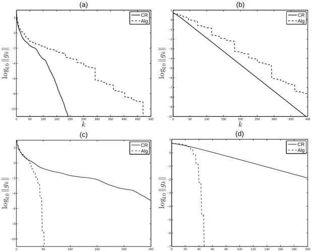
Example 3 In this artificial example, A is diagonal with m = 1, M = 1 000, n = 1 000 and b = Ac with c random (uniformly distributed on the unit n-dimensional sphere Sn). We
consider two configurations for the eigenvalues of A and starting point x0. In the first case, the
n eigenvalues are uniformly distributed in [m, M ] and x0 is random (uniformly distributed on
Sn). The second configuration corresponds to the worst-case situation for n − 1 steps of the Conjugate Residual (CR) algorithm: the eigenvalues are
λi = (M + m)/2 + (M − m)/2 cos[π(i − 1)/(n − 1)] for i = 1, . . . , n
and x0 is such that the α2i in the decomposition (9) are proportional to τ12 = 1/2λ1, τj2 = 1/λj
for j = 2, . . . , n − 1 and τn2 = 1/2λn, see [15] for details. Figures 3(a) and 3(b) present the
evolution of log10kgkk as a function of k for the algorithm above (Alg) and the CR algorithm
not competitive in this respect. On the other hand, the evolution of log10kgkk as a function of
the number of inner products computed is plotted in Figures 3(c) and 3(d), showing the gain in complexity of the proposed algorithm compared to CR.
0 50 100 150 200 250 300 350 400 450 500 −10 −8 −6 −4 −2 0 2 k lo g10 k gk k (a) CR Alg 0 50 100 150 200 250 300 350 400 −10 −9 −8 −7 −6 −5 −4 −3 −2 −1 0 1 k lo g10 k gk k (b) CR Alg 0 50 100 150 200 250 −10 −8 −6 −4 −2 0 2 lo g10 k gk k (c) CR Alg 0 20 40 60 80 100 120 140 160 180 200 −7 −6 −5 −4 −3 −2 −1 0 1 lo g10 k gk k (d) CR Alg
Figure 3: log10kgkk as a function of k (top), log10kgkk against the number of inner products
computed (bottom) in Example 3. The eigenvalues of A are uniformly distributed in [m, M ] = [1, 1 000] in (a) and (c); (b) and (d) correspond to the worst-case situation for the CR algorithm.
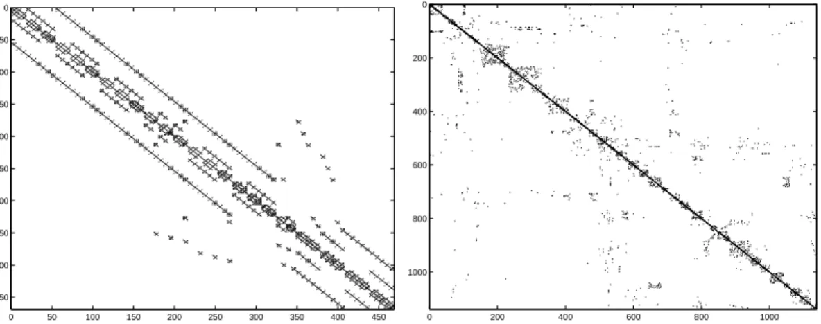
Example 4 A is given by the matrix NOS5 from http://math.nist.gov/MatrixMarket/; it is sparse, with dimension n = 468 and N = 5 172 non-zero elements only, its structure is shown in Figure 4 (left). Its condition number approximately equals 1.1 · 104.
Example 5 A is given by the matrix 1138 BUS from http://math.nist.gov/MatrixMarket/; this matrix is also sparse and symmetric positive-definite with n = 1 138 and N = 4 054 non-zero elements, see Figure 4 (right). Its condition number approximately equals 1.5277 · 105.
We set b = Ac, c and x0 are uniformly distributed on Sn. Figure 5 presents the evolution of
log10kgkk against the number inner products in Examples 2 and 3, computed for the algorithm
above (Alg) and the CR algorithm. The reduced complexity of the proposed algorithm compared to CR is manifest.
0 50 100 150 200 250 300 350 400 450 0 50 100 150 200 250 300 350 400 450 0 200 400 600 800 1000 0 200 400 600 800 1000
Figure 4: Non-zero elements of A in Examples 4 (left) and 5 (right).
0 50 100 150 200 250 300 350 −6 −4 −2 0 2 4 6 lo g1 0 k gk k CR Alg 0 50 100 150 200 250 300 350 400 450 500 −3 −2 −1 0 1 2 3 4 lo g1 0 k gk k CR Alg
Figure 5: log10kgkk against the number of inner products computed in Examples 4 (left) and 5
(right).
6
Proofs
Proof of Lemma 1.
Since { bmk} forms a non-increasing sequence bounded from below by m, bmk→ m∞as k → ∞ for some m∞≥ m.
Similarly, cMk → M∞ for some M∞ ≤ M. Denote ǫ1 = m∞− m, ǫ2 = M − M∞, ǫ1, ǫ2 ≥ 0. Suppose that
0 ≤ ǫ1< ǫ2. Then, the asymptotic distribution of the sequence {βk} is biased towards m. From (11), the sequence
{νk} tends to concentrate at M so that cMk→ M as k → ∞, implying ǫ2= 0, which contradicts the assumption
0 ≤ ǫ1< ǫ2. Similarly, the assumption ǫ1> ǫ2≥ 0 leads to a contradiction; therefore, M − M∞= m∞− m.
Proof of Th. 2.
From Lemma 1, m∞= m + ǫ and M∞= M − ǫ for some ǫ ≥ 0. Assuming that ǫ > 0, we show that this leads
to a contradiction. The proof is in two steps. In (i) we show that bmkis repeatedly updated; in (ii) we show that
this implies m∞= m and thus ǫ = 0.
(i) We have from (11)
p(k+1)1 p(k+1)d = (βk− m)2 (M − βk)2 p(k)1 p(k)d .
0 ≤ δk≤ Dθk when k > k0 for some k0, D > 0 and 0 ≤ θ < 1. Denoting pk= p(k)1 , Qk= pk/(1 − pk), we get Qk+1= pk+1 (1 − pk+1) = Qk (βk− m)2 (M − βk)2 1 − δk+1 1−pk+1 1 − δk 1−pk . (27)
Since m + ǫ ≤ µ(k)1 ≤ M − ǫ for all k, we have
ǫ M − m− Bθ k ≤ pk≤ 1 − ǫ M − m+ Bθ k
for some B > 0 when k > k0. Therefore, 1−pk> ǫ/[2(M −m)] for k large enough and, together with 0 ≤ δk≤ Dθk,
(27) gives
log Qk+1= log Qk+ log
µ βk− m
M − βk
¶2
+ ck,
with |ck| < Cθk for all k larger than some k1, C = 4D(M − m)/ǫ. This implies that
¯ ¯ ¯ ¯ ¯ ¯log Qk+1 Qk1 − k X j=k1 log µ βj− m M − βj ¶2¯¯¯ ¯ ¯ ¯< ∞ X j=0 Cθj< C 1 − θ. (28) Denote ξj= log µ βj− m M − βj ¶2 .
Suppose that there is no update of bmk and cMkafter some k2 and denote ǫm= bmk2− m, ǫM = M − cMk2. Then, for j > k2, {ξj} forms a sequence of i.i.d. random variables and (28) indicates that, for k > k2, log Qk+1− log Qk2 behaves like a random walk. The random variables ξj have mean
M (ǫm, ǫM) = Z log à t + 1 + 2ǫm M −m−ǫm−ǫM 1 + 2ǫM M −m−ǫm−ǫM − t !2 .
From Lemma 1, ǫm= ǫM = ǫ. Since M (ǫ, ǫ) = 0, the random walk has no drift and we have lim supk→∞log Qk=
− lim infk→∞log Qk = ∞ a.s., which contradicts the assumption of no update of bmk and cMk after iteration k2.
(One may notice that ξ2j+ ξ2j+1= 0 when the βkare generated according to (16), so that the argument cannot
be used in that case.)
Suppose now that there is no update of bmk for k > k2 and denote ǫm = bmk2− m. From the argument above, cMk is repeatedly updated, which, from Lemma 1, is only possible if ǫM,k = M − cMk > ǫm. The ξj, for
j > k2, are now neither independent nor identically distributed, but IE(ξj|Fj−1) = M (ǫm, ǫM,j) < 0, with {Fj}
the sequence of σ-fields σ(α0, α1, . . . , αj). From (28), the sequence of log Qk+1− log Qk2, k > k2, thus forms a
supermartingale relative to {Fj}. Consider now Sk=
Pk
j=k2ξj−IE(ξj|Fj−1), which forms a martingale sequence. Since we assume that ǫ > 0, the increments |ξj− IE(ξj|Fj−1)| are bounded and Sk/
√
k satisfies the central limit theorem (see, e.g., [6]). This implies that lim infk→∞log Qk = −∞ and therefore M∞ = M , which contradicts
the assumption of ǫ > 0. We have thus proved that bmkis updated infinitely often.
(ii) Similarly to (i), m∞= m + ǫ and M∞= M − ǫ with ǫ > 0, βksatisfying (15) with Fα(·) satisfying (20) imply
that (19) is satisfied. Denoting pk= p(k)1 , direct calculations using (11) and (12) give
pk+1≥ · 1 −1 + 4p1 − pk kωk ¸ + Dθk (29)
when k > k0, for some constants D ≤ 0 and 0 ≤ θ < 1, where ωk= ζk/(1−ζk)2with ζk= [βk−(M +m)/2]/[(M −
m)/2] and βk∈ (m + ǫ, M − ǫ) by construction. (Notice that the term within square brackets on the right-hand
side of (29) is an increasing function of both pkand βk.) The fact that Fα(1 − x) < 1 for any x > 0 implies that
lim supk→∞βk= M − ǫ. We have shown in (i) that bmkis updated infinitely often. Therefore, for any δ1, δ2> 0,
there exists a subsequence {ji} such that βji > M − ǫ − δ1 and µ
(ji)
1 < m + ǫ + δ2. For a two-point measure
supported at m and M , this second inequality implies pji> (M − ǫ − m)/(M − m) − δ3, with δ3→ 0 as δ2→ 0. Due to Th. 1, we thus have
pji>
M − m − ǫ
M − m − δ3+ Bθ
ji for some constant B ≤ 0 and all ji> k0. Together with (29), it gives
pji+1>
(M − m − ǫ)3
where δ4 can be made arbitrarily small by taking δ1, δ2 small enough and i large enough. This implies that
µ(ji+1)
1 < m + ǫ + δ5−ǫ(M − m − ǫ)(M − m − 2ǫ)
(M − m)2− 3ǫ(M − m − ǫ) < m + ǫ
for δ1, δ2 small enough and i large enough, which contradicts m∞= m + ǫ.
Proof of Th. 3.
The proof is similar to part (ii) of the proof of Th. 2. From Lemma 1, m∞= m + ǫ and M∞= M − ǫ for some
ǫ ≥ 0. Suppose that ǫ > 0. When βk satisfies one of the rules (15-17) with Fα(·) satisfying (20), then (19) is
satisfied which implies (29) for k > k0 and some constants D ≤ 0 and 0 ≤ θ < 1, where ωk= ζk/(1 − ζk)2 with
ζk= [βk− (M + m)/2]/[(M − m)/2] and βk∈ (m + ǫ, M − ǫ) by construction. Since M∞= M − ǫ, (13) implies
that µ(k)2 /µ(k)1 ≤ M − ǫ. For a two-point measure supported at m and M, this implies pk≥ Mǫ/[(M − m)(m + ǫ)];
in view of Th. 1, we thus have
pk≥
M ǫ
(M − m)(m + ǫ)+ Bθ
k
(30) for some constant B ≤ 0 and k > k0. Since Fα(1 − x) < 1 for any x > 0, lim supk→∞βk = M − ǫ and, for any
δ1> 0 and any k1, there exist some k > k1 such that βk> M − ǫ − δ1. In view of (29) and (30) this implies that
pk+1≥ M (M − m − ǫ)
(M − m)(M − ǫ)− δ2
where δ2can be made arbitrarily small by taking δ1 small enough and k1large enough. This implies in turn that
µ(k+1)1 ≤ M m
M − ǫ+ δ3= m + ǫ + δ3−
ǫ(M − m − ǫ)
M − ǫ < m + ǫ for δ1 small enough and k1 large enough, which contradicts m∞= m + ǫ with ǫ > 0.
Proof of Th. 5.
Following the same arguments as in the proof of Th. 3, (30) implies that µ(k+1)1 < m + ǫ for δ < δǫand k large
enough, with δǫ= 2ǫ(√M m − m − ǫ)(M − m − ǫ) [M m − (m + ǫ)2](M − m − 2ǫ) = 2ǫ √m(√ M +√m)+ O(ǫ 2) .
From this we obtain that for small δ, 0 ≤ m∞− m = M − M∞ ≤
√
m(√M +√m)δ/2 + O(δ2), so that the βk
are asymptotically distributed in [m + ǫ′
, M − ǫ′
] with ǫ′
satisfying (25). (Note that m + ǫ′′
≤ βk ≤ M − ǫ ′′
for all k, with ǫ′′
= δ(M − m)/2.)
The conditions of Th. 1 are satisfied, so thatPn−1i=2 νk(λi) ≤ Cθk for k > 2j0for some constants C > 0, j0> 0
and 0 ≤ θ < 1. Also, accounting for the fact that the distribution of β2j is not exactly symmetric in [m, M ], for
any δ1> 0 there exists some j1 such that for all j > j1, |r2jr2j+1− R22(β2j)| < δ1. Altogether, for j > j1 large
enough,
R22(β2j) − Dθ2j− δ1< r2jr2j+1 < R22(β2j) + Dθ2j+ δ1 (31) for some D > 0. Since β2j, β2j+1 ∈ [m + ǫ
′′ , M − ǫ′′ ] for all k, R2(β2j) > R2(m + ǫ ′′ ) = R2(M − ǫ ′′ ) = ǫ′′ (M + m − ǫ′′ )/[(m + ǫ′′ )(M − ǫ′′ )] > 0 and
2 log[R2(β2j)] − δ2< log(r2jr2j+1) < 2 log[R2(β2j)] + δ2
for j > j1, where δ2 can be made arbitrarily small by taking j1 large enough. From the definition (6) of Rk, we
can thus write 1 2(i − j1) log µ R2i R2j1 ¶ = 1 2(i − j1) i−1 X j=j1 log(r2jr2j+1) = 1 (i − j1) i−1 X j=j1 log[R2(β2j)] + C with |C| < δ2/2. Therefore, lim k→∞ 1 klog Rk= Z log(1 − α + 2ǫ′ M −m−2ǫ′)(1 + α + 2ǫ′ M −m−2ǫ′) ³ M+m M −m−2ǫ′ ´2 − α2 dFα(t) for some ǫ′
References
[1] J. Barzilai and J.M. Borwein. Two-point step size gradient methods. IMA J. Numer. Anal., 8:141–148, 1988.
[2] P. Embrechts, C. Kl¨uppelberg, and T. Mikosch. Modelling Extremal Events. Springer, Berlin, 1997.
[3] B. Fischer and L. Reichel. A stable Richardson iteration method for complex linear systems. Numer. Math., 54:225–242, 1988.
[4] G. E. Forsythe. On the asymptotic directions of the s-dimensional optimum gradient method. Numer. Math., 11:57–76, 1968.
[5] G.H. Golub and C.F. Van Loan. Matrix Computations. Johns Hopkins University Press, third edition, 1996.
[6] P. Hall and C.C. Heyde. Martingale Limit Theory and Its Applications. Academic Press, New York, 1980.
[7] M. H. Hestenes and E. Stiefel. Methods of conjugate gradients for solving linear systems. J. Res. Nat. Bur. Stand., 49:409–436, 1952.
[8] M.A. Krasnosel’skii and S.G. Krein. An iteration process with minimal residues. Mat. Sb. (in Russian), 31(4):315–334, 1952.
[9] G. Meurant. The block preconditioned conjugate gradient method on vector computers. BIT, 24:623–633, 1984.
[10] H. Niederreiter. Random Number Generation and Quasi-Monte Carlo Methods. SIAM, Philadelphia, 1992.
[11] C.C. Paige and M.A. Saunders. Solution of sparse indefinite systems of linear equations. SIAM J. Numer. Anal., 12(4):617–629, 1975.
[12] O.M. Podvigina and V.A. Zheligovsky. An optimized iterative method for numerical solu-tion of large systems of equasolu-tions based on the extremal property of zeros of Chebyshev polynomials. J. of Scientific Computing, 12(4):433–464, 1976.
[13] L. Pronzato, H.P. Wynn, and A. Zhigljavsky. Renormalised steepest descent in Hilbert space converges to a two-point attractor. Acta Appl. Math., 67:1–18, 2001.
[14] L. Pronzato, H.P. Wynn, and A.A. Zhigljavsky. Asymptotic behaviour of a family of gradient algorithms in Rd and Hilbert spaces. Mathematical Programming, A107:409–438, 2006.
[15] L. Pronzato, H.P. Wynn, and A.A. Zhigljavsky. A dynamical-system analysis of the opti-mum s-gradient algorithm. In L. Pronzato and A.A. Zhigljavsky, editors, Optimal Design and Related Areas in Optimization and Statistics, chapter 3, pages 39–80. Springer, 2009. [16] L. Pronzato and A. Zhigljavsky. Gradient algorithms for quadratic optimization with fast
[17] Y. Saad. Practical use of polynomial preconditionings for the conjugate gradient method. SIAM J. Sci. Stat. Comp., 6(4):865–881, 1985.
[18] Y. Saad. Iterative Methods for Sparse Linear Systems. Society for Industrial and Applied Mathematics, 2008.
[19] B. Slater. Gaps and steps for the sequence n θ mod 1. Math. Proc. Camb. Phil. Soc., 63:1115–1123, 1967.
[20] H. Tal-Ezer. Polynomial approximation of functions of matrices and applications. J. of Scientific Computing, 4(1):25–60, 1989.
[21] H.A. van der Vorst. Iterative Methods for Large Linear Systems. Utrecht University, Utrecht, 2000.
[22] A. Zhigljavsky, L. Pronzato, and E. Bukina. An asymptotically optimal gradient algorithm for quadratic optimization with low computational cost. Optimization Letters, 2012. (DOI 10.1007/s11590-012-0491-7, to appear).
![Figure 2: Rate R 1/2i 2i as a function of i for α k = cos(π[(k + 1)ϕ mod 1]) for all k ≥ 0 (solid line) and for { α k } a random i.i.d](https://thumb-eu.123doks.com/thumbv2/123doknet/13633454.426683/14.892.279.616.117.375/figure-rate-function-cos-mod-solid-line-random.webp)