HAL Id: insu-01382419
https://hal-insu.archives-ouvertes.fr/insu-01382419
Submitted on 17 Oct 2016
HAL is a multi-disciplinary open access archive for the deposit and dissemination of sci-entific research documents, whether they are pub-lished or not. The documents may come from teaching and research institutions in France or abroad, or from public or private research centers.
L’archive ouverte pluridisciplinaire HAL, est destinée au dépôt et à la diffusion de documents scientifiques de niveau recherche, publiés ou non, émanant des établissements d’enseignement et de recherche français ou étrangers, des laboratoires publics ou privés.
Bayesian network
Pedram Masoudi, Yousef Asgarinezhad, Behzad Tokhmechi
To cite this version:
Pedram Masoudi, Yousef Asgarinezhad, Behzad Tokhmechi. Feature selection for reservoir character-isation by Bayesian network. Arabian Journal of Geosciences, Springer, 2015, 8 (5), pp.3031-3043. �10.1007/s12517-014-1361-7�. �insu-01382419�
Feature selection for reservoir characterisation by Bayesian Network
Pedram Masoudi1*, Yousef Asgarinezhad2, Behzad Tokhmechi2
1
Presently, PhD Student and Researcher of Petroleum Geoscience at School of Mining Eng., University College of Engineering (Fanni), University of Tehran. Formerly, Researcher of
Petroleum Geoscience at Department of Research and Technology, Iranian Offshore Oil Company (IOOC), Tehran, Iran
2
School of Mining, Petroleum and Geophysics Engineering, University of Shahrood, Shahrood, Iran
*Corresponding author (E-mail: [email protected])
Abstract
The more accurate feature identification, the more precise reservoir characterisation.
Porosity, permeability and other rock properties could be estimated and classified by analytical
and intelligent methods. Feature selection, plays a vital role in the process of identification. In
this work, two goals are followed: first, developing Bayesian Network, K2 algorithm, as a
complementary means (not an alternative) to find interrelationships of petrophysical parameters.
Second, feature conditioning for estimating porosity and permeability, vug and fracture
detection, and net pay determination. Due to the results, bulk density log is introduced as the
most important feature for characterising the reservoir because it is found useful for identifying
all the studied reservoir features.
Keywords: feature conditioning; porosity; permeability; fracture; vug; net pay
1. Introduction 1 2 3 4 5 6 7 8 9 10 11 12 13 14 15 16 17 18 19 20 21 22 23 24 25 26 27 28 29 30 31 32 33 34 35 36 37 38 39 40 41 42 43 44 45 46 47 48 49 50 51 52 53 54 55 56 57 58 59 60 61
The concept of Bayesian Network (BN) was firstly developed in the fields of electrical
and computer engineering. (Pearl, 1986) and (Cooper and Herskovits, 1992) are of pioneers in
Bayesian Network (BN) who defined this concept, and introduced the methodology clearly and
applicably at the time. Later on, this methodology was used in a wide range of science and
technology. (Doguc and Ramirez-Marquez, 2009) utilized BN in estimating system reliability.
Khor et al constructed three different types of BN classifiers in detecting network attacks; and by
comparing the results, they concluded that these three types are well equivalent in performance
(Khor et al., 2009). BN is also used in some other fields like forecasting price in stock market
(Zuo and Kita, 2012). It is some years that BN has been entered in geoscience studies. Based on
the records of Scopus database; among all fields of earth science, remote sensing benefits from
BN the most.
In petroleum industry, BN is used to assess situations and conditions probabilistically,
e.g. in downstream it is used in circulation monitoring system (Mansure et al., 1999); safety
instrumentation and risk reduction at wellsite (Kannan, 2006); identifying candidate wells for
gel-polymer treatment (Ghoraishy et al., 2008); drilling industry (Al-yami and Schubert, 2012;
Al-Yami et al., 2010; Rajaieyamchee and Bratvold, 2009); production issues and history
matching (Abdollahzadeh et al., 2011; Hermann et al., 2011; Khaz'ali et al., 2011); completion
(Al-yami et al., 2011); and Enhanced Oil Recovery (EOR) (Zerafat et al., 2011)
There are some publications of application of BN in upstream, specifically in basin
analysis from economical evaluation of prospects (Van Wees et al., 2008) to studying
dependency relationships between geological features (Martinelli et al., 2011; Martinelli et al.,
2013; Rasheva and Bratvold, 2011). In addition, there are two recently published papers in the
4 5 6 7 8 9 10 11 12 13 14 15 16 17 18 19 20 21 22 23 24 25 26 27 28 29 30 31 32 33 34 35 36 37 38 39 40 41 42 43 44 45 46 47 48 49 50 51 52 53 54 55 56 57 58 59
upstream that have used BN in identifying effective logs, i.e. feature selection for determining
productive zones through oil wells. Due to the results of one of articles, the ratio of LLD to LLS
and individually LLD are the most effective raw features for detecting productive zones through
oil wells (Masoudi et al., 2012c). Based on the results of the latter, porosity and water saturation
are the most important extracted features for evaluating productive zones (Masoudi et al.,
2012a).
It is worthy to mention that feature selection/ extraction is a basic and important stage in
the process of identification (Russo and Ramponi, 1994). It is not a good idea to consider all
available information as input parameters. In another words, redundant information or
duplications should be detected and removed from dataset (Bleiholder and Naumann, 2008).
The mentioned literature review reveals that newly developed concept of BN in
petroleum industry is gradually going to become more and more applicable and renowned in
exploratory investigations. As BN is a powerful tool to identify causal relationships between
different features and phenomena, we have utilized it as a means to select effective petrophysical
features for reservoir identification. The proposed procedure is based on correlation and
dependency relations between reservoir properties and petrophysical parameters. In fact, we
think that the deeper and the more precise understanding of interrelations and causations between
parameters, the more effective feature selection, which plays an important role in success of any
identification procedure; i.e. estimation, classification or clustering. Therefore, in this paper,
authors follow two aims; the first one is developing the concept of dependency and Bayesian
Network as an intelligent methodology for finding causality relationships and feature selection in
petrophysical assessments, which is the novelty of this article. Second goal is introducing useful
4 5 6 7 8 9 10 11 12 13 14 15 16 17 18 19 20 21 22 23 24 25 26 27 28 29 30 31 32 33 34 35 36 37 38 39 40 41 42 43 44 45 46 47 48 49 50 51 52 53 54 55 56 57 58 59 60 61
petrophysical parameters for identifying some reservoir properties (porosity, permeability, open
fractures, vuggy porosity and net pay) within oil wells, which is a practical aid for
petrophysiscists and geoscientists in their studies.
To do so, a brief review on a famous feature selection criterion, correlation coefficient, is
presented following introducing available datasets; then, concept of “dependency” and methodology of “Bayesian Network” are added to make respected readers familiar with the concept and methodology. Thereafter, generated BNs and their outputs in various aspects of
reservoir characterisation (estimating porosity and permeability, vug and fracture detection, and
net pay determination) are included, followed by discussion and conclusion.
2. Datasets
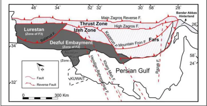
In this work, petrophysical datasets of three Iranian oil-fields in Zagros Region have been
studied. For the sake of confidentiality of data and information in National Iranian Oil Company
(NIOC), the names of oil-fields under study (F1, F2 and F3) have not been enclosed but their
approximate locations are indicated on Fig. 1.
4 5 6 7 8 9 10 11 12 13 14 15 16 17 18 19 20 21 22 23 24 25 26 27 28 29 30 31 32 33 34 35 36 37 38 39 40 41 42 43 44 45 46 47 48 49 50 51 52 53 54 55 56 57 58 59
Fig. 1. Map of Zagros Region and main faults of the region. Modified after (Masoudi et al.,
2012b; Rajabi et al., 2010; Sherkati and Letouzey, 2004).
F1 is a giant field in Abadan Plain with North-South trend that has been used for
evaluating net pay zones and estimating porosity and permeability. In this field, Sarvak
Formation (Albian to Turonian) in six exploratory wells is studied. For fracture detection, one oil
well in another giant oil-field (F2) is chosen. F2 is a Northwest- Southeast anticline in northern
side of Kazerun Fault in South Dezful Area, very close to Izeh Zone. The reason why this field is
selected for fracture study is availability of interpreted image logs and fullest of petrophysical
data. For vug detection, a relatively small-sized anticline-shaped field (F3) in central Lurestan
Area is selected. Access of authors to studied core reports is the reason for selecting this field to
find causal relationship of vuggy porosity with petrophysical data. F3 has the same trend as F2,
and like F1, investigation is fulfilled again within Sarvak Formation. Whereas the approximate
4 5 6 7 8 9 10 11 12 13 14 15 16 17 18 19 20 21 22 23 24 25 26 27 28 29 30 31 32 33 34 35 36 37 38 39 40 41 42 43 44 45 46 47 48 49 50 51 52 53 54 55 56 57 58 59 60 61
locations could be seen in Fig. 1; summary of data and the purpose of choosing these three fields
is summarized in Table 1.
Summary of available data and information in F1 are shown in Table 2. CGR, DT, NPHI,
RHOB, LLD, LLS and MSFL are common well logs in all six wells; therefore, in order to
incorporate maximum number of wells, other well logs are not included in this study. In addition,
because there is no core data in well 6, this well is exempted from porosity- permeability study.
Also, due to lack of well test data in well 5, this well is exempted from net pay investigation.
In each of F2 and F3 fields, only one well is available. Available data in F2 are CGR,
NPHI, DT, PEF, RHOB and SGR well logs, and interpretation of open fractures on image log;
whereas available data in F3 are GR, Cali, RHOB, DRHO, NPHI, DT and LLD well logs, and
observed vuggy porosity in cores.
3. A Simple Review of the Correlation Coefficient
Correlation coefficient is a well-known factor, measuring correlation (mutual
relationship) between two different variables. There are different standpoints for calculating
correlation coefficient: algebraic, geometric, and trigonometric. Pearson product-moment
correlation coefficient is the most well-known formula for calculating correlation coefficient of
two variables from algebraic viewpoint (Lee Rodgers and Nicewander, 1988). Fig. 2 shows two
correlated variables; i.e. b changes when a changes in the same or reverse direction (variables in
Fig. 2 are correlated in the same direction). Although correlation coefficient is a very valuable
and important factor for understanding interrelations of variables, there are some insufficiencies
in using it (Bobko, 2001). 4 5 6 7 8 9 10 11 12 13 14 15 16 17 18 19 20 21 22 23 24 25 26 27 28 29 30 31 32 33 34 35 36 37 38 39 40 41 42 43 44 45 46 47 48 49 50 51 52 53 54 55 56 57 58 59
Fig. 2. The more correlated variables (here a and b), the closer dots to the dashed line.
One easy-understanding example for showing insufficiency of correlation coefficient is in
describing causal relationship between father and son. If the number of adults rises in a city, it
does not necessarily mean that the number of children has risen too (Whereas Population Growth
Rate is positive in developing countries, it is very close to zero or even negative in developed
countries, and is not directly related to number of fathers or adults). But when the number of kids
rises, you are 100% sure that the number of fathers (adults) has risen; because every kid needs a
father to be born but fathers do not need their children for existing! Therefore, there is no mutual
relation or correlation between number of fathers and children; however one of them is
dependent on the other (directional relation).
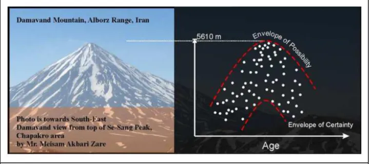
Another example for insufficiency of correlation coefficient in showing interrelation of
two variables, revealed in Fig. 3. If 100 people are asked to climb Damavand Mountain (highest
peak in Iran with elevation of 5610 meters above the geoid), and plot the height of which they
have reached against their ages, the plot would be like in Fig. 3. In fact, the acquired data is
distributed between two envelopes that show possible and certain accessible heights for each age.
The shapes of these two envelopes are similar to an inverse “V”, because teenagers and olds are
4 5 6 7 8 9 10 11 12 13 14 15 16 17 18 19 20 21 22 23 24 25 26 27 28 29 30 31 32 33 34 35 36 37 38 39 40 41 42 43 44 45 46 47 48 49 50 51 52 53 54 55 56 57 58 59 60 61
not able in reaching high heights, whereas young people and middle-aged can even reach the
peak. Correlation coefficient of dataset of this plot is something close to zero but without any
shadow of doubt, there is a relationship between maximum accessible height and age in
mountain climbing, while they are not correlated due to correlation coefficient.
Fig. 3. Dependency between age and accessible height for a man.
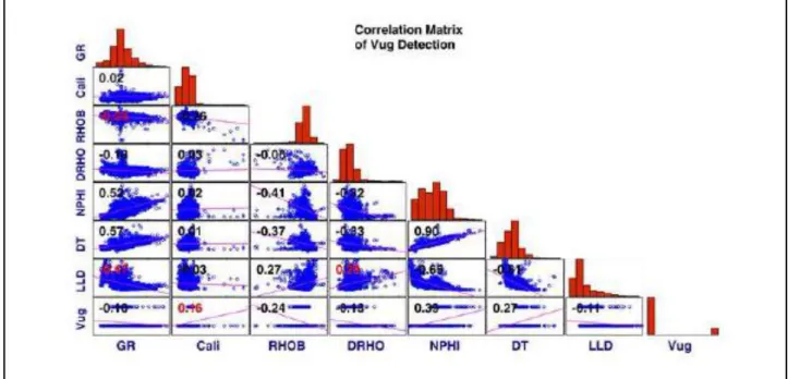
A practical example of this inefficiency in petrophysics could be found on cross-plot of
Calliper-Vug and RHOB-Vug on Fig. 8. In these two cross-plots, there is no mutual relationship
between two plotted variables as in Fig. 3, later we show that both Calliper and RHOB are
important features for vug detection.
4. What Is Dependency?
This work introduces dependency between variables as an alternative for finding related
variables, especially when there is no mutual relationship like relationship of father and child.
Now, what is dependency? Each field has its own definition of dependency, and they are close to
4 5 6 7 8 9 10 11 12 13 14 15 16 17 18 19 20 21 22 23 24 25 26 27 28 29 30 31 32 33 34 35 36 37 38 39 40 41 42 43 44 45 46 47 48 49 50 51 52 53 54 55 56 57 58 59
each other. Oxford dictionary states that “dependence” means “the state of relying on or being
controlled by someone or something else” (OxfordDictionaries, 2010). From mathematical viewpoint, probabilistic is a means for evaluating dependency of variables on each other.
Probabilistically, two variables are called independence, when the joint probability of them is
equal to product of their own probability (Olofsson, 2011):
(1)
In the above equation, A and B are independent sets. Bayesian Probability is theory of
studying conditional probability between two or more dependent variables, which uses Bayes
rule for calculating evidential probabilities (Duda et al., 2000). Bayesian Network, which is
introduced here in order to find out dependency relation between petrophysical variables, is
mainly based on Bayesian theory of conditional probabilities.
5. Methodology
5.1. Bayesian Network
Consider five measured variables (named a1 to a6) that are supposed to be effective on
another unknown variable, called b, and each of these seven parameters can admit four different
states. Therefore there are four powered seven (i.e. 16’384) possible states, and it is not only hard to compute and consider all these states (an NP-hard problem), but also impossible in the case of
lack of complete and comprehensive dataset of records.
Bayesian Network is a directed acyclic graph that nodes represent variables and edges
show direct dependencies between the linked variables. Now, suppose that dependency
4 5 6 7 8 9 10 11 12 13 14 15 16 17 18 19 20 21 22 23 24 25 26 27 28 29 30 31 32 33 34 35 36 37 38 39 40 41 42 43 44 45 46 47 48 49 50 51 52 53 54 55 56 57 58 59 60 61
relationships between those previously mentioned seven variables can be represented as in Fig.
4. Based on this graph, the variable b is only dependent on the variables a3, a4 and a5. Also, it is
simple to formulate probability of b as:
(2)
(3)
That P(x) is probability of occurrence of x, is joint probability, i.e. probability
of occurrence of x and y simultaneously, is probability of x, considering y, i.e.
conditional probability. The first equation is inferred from independency of the variable a5 and set of variables a3 and a4. For better understanding of equation 3, respected readers are referred to
(Pearl, 1986).
Fig. 4. A Bayesian Network, showing dependency relation of seven variables of a1 to a6 and b. 4 5 6 7 8 9 10 11 12 13 14 15 16 17 18 19 20 21 22 23 24 25 26 27 28 29 30 31 32 33 34 35 36 37 38 39 40 41 42 43 44 45 46 47 48 49 50 51 52 53 54 55 56 57 58 59
There are two methodologies for constructing BNs: constraint-based methods and
score-based methods (Lauría, 2008). The former is used in cases that user is confident about the causal
relationships between variables. For instance Total Organic Carbon (TOC) is a prerequisite for
oil generation, and none of specialists believe that oil could be generated without having some
least amount of TOC (Al-Ameri et al., 2009). Furthermore there is a dependency relation
between TOC and oil generation. In fact, constraint-based methods are judgmental methods that
an expert is responsible for (Martinelli et al., 2011).
In some cases, it is difficult or even impossible for a user to determine dependency
relations between variables. In these cases, data-driven approaches are used to find the most
probable state of dependency between each pair of variables. In score-based methods, a
calculated score is set as a criterion to find the dependency relation between two variables. For
using score-based methods, two elements should be specified: search procedure and scoring
metric. Scoring function should be associated with probability of a candidate directed acyclic
graph, and search procedure is considered as an optimization problem. Greedy hill-climbing
algorithm, K2 algorithm, simulated annealing optimization, Monte Carlo are some of those
score-based methods, known as heuristic approaches to construct a BN (Cooper and Herskovits,
1992; Lauría, 2008; Niedermayer, 2008). In this work, K2 algorithm is used in order to construct
BNs.
5.2. K2 Algorithm
K2 algorithm is a score-based method for constructing BNs, although it is not completely
free of constraint. Two constraints should be considered prior to running K2 algorithm. The first
one is to state the maximum possible parents that each node can have; the other is providing a
4 5 6 7 8 9 10 11 12 13 14 15 16 17 18 19 20 21 22 23 24 25 26 27 28 29 30 31 32 33 34 35 36 37 38 39 40 41 42 43 44 45 46 47 48 49 50 51 52 53 54 55 56 57 58 59 60 61
true initial order of variables by user that variables are not dependent in reverse order. E.g. if the
initial order of (a1, a2, a3, … , an) is provided by user, aj could be dependent on ai (i<j); though ai cannot be dependent on aj but if ai and aj are mutually correlated. After considering these two
constraints, following algorithm should be applied on the dataset (Doguc and Ramirez-Marquez,
2009):
Algorithm K2(T,u):
Input: dataset of observations, T, and maximum possible number of parents for each node, u.
Output: Bayesian Network, BN.
(1) For each variable in input dataset, T
(1-1) Create node Ai as i-th variable, and add it to BN
(1-2) Create an empty set as set of parents (Pai) of Ai
(1-3) Calculate by:
(4)
Where, is number of times that Ai and Aj are in a specific state of k. di is number of
states of Ai. Finally, qi is number of possible parents, i.e. .
4 5 6 7 8 9 10 11 12 13 14 15 16 17 18 19 20 21 22 23 24 25 26 27 28 29 30 31 32 33 34 35 36 37 38 39 40 41 42 43 44 45 46 47 48 49 50 51 52 53 54 55 56 57 58 59
(1-4) While number of elements of Pai is not larger than u:
(1-4-1) Assume Xz as a parental node of Xi
(1-4-2) Calculate
(1-4-3) If the score of is larger than , fix Az as a
permanent node of Ai, otherwise, remove it from parental set (Pai).
(2) Return BN
6. Results
In this section, correlation coefficient and Bayesian Network are utilized to find out
effective features for reservoir identification. In the first part, important features for porosity and
permeability estimation are determined, and in the second, third and fourth parts, useful features
for fracture and vug detection and net pay assessment are determined respectively.
6.1. Causal Relationships in Porosity and Permeability Estimation
Estimating porosity and permeability of reservoir rocks is very essential in reservoir
characterization, static and dynamic modelling. There are many investigations about estimating
porosity and permeability of reservoirs. The input features, used for estimating these two
parameters have not remained unchanged during time. Table 3 shows different datasets,
introduced for porosity and permeability estimation in chronological order.
4 5 6 7 8 9 10 11 12 13 14 15 16 17 18 19 20 21 22 23 24 25 26 27 28 29 30 31 32 33 34 35 36 37 38 39 40 41 42 43 44 45 46 47 48 49 50 51 52 53 54 55 56 57 58 59 60 61
In order to find out, appropriate features for estimating porosity and permeability, scatter
plots of all logs, and porosity and permeability of core analysis are plotted on Fig. 5 (a) and (b).
Then, correlation coefficients between each pair of variables are calculated and shown on each
plot. Thereafter, Bayesian Network (Fig. 5 (c)) is constructed by K2 algorithm with the order of:
CGR, NPHI, RHOB, DT, LLD, MSFL, LLS, LLD/LLS, Porosity, Log(Perm)
Lognormal distribution of permeability is the reason why permeability is used in
logarithmic scale. It is reported that it would be much better to estimate logarithm of
permeability instead of raw permeability to have a more precise estimation of body (not
extremes) of permeability values (Masoudi et al., 2011a).
(a) Correlation Coefficients and histograms (Part I: lithologic well logs)
4 5 6 7 8 9 10 11 12 13 14 15 16 17 18 19 20 21 22 23 24 25 26 27 28 29 30 31 32 33 34 35 36 37 38 39 40 41 42 43 44 45 46 47 48 49 50 51 52 53 54 55 56 57 58 59
(b) Correlation Coefficients and histograms (Part II: resistivity well logs)
(c) Bayesian Network
Fig. 5. Relationships between features in Sarvak Formation of F1 for porosity and permeability
estimation.
Due to criterion of correlation coefficient, porosity is relatively well-correlated to
Log(Perm) and RHOB. Based on constructed BN, porosity is related to Log(Perm) (child) and
4 5 6 7 8 9 10 11 12 13 14 15 16 17 18 19 20 21 22 23 24 25 26 27 28 29 30 31 32 33 34 35 36 37 38 39 40 41 42 43 44 45 46 47 48 49 50 51 52 53 54 55 56 57 58 59 60 61
RHOB (parent) in the first order. Therefore, both criteria, unanimously agree that the first two
features, related to porosity are Log(Perm) and RHOB. Again due to correlation coefficient,
Log(Perm) is relatively well-correlated with porosity and LLD. BN approves that porosity is the
most influential factor for estimating Log(Perm), whereas defines RHOB in the second stage.
It is relatively easy to come on an agreement in feature selection for porosity because
priorities of both criteria are very close to each other. Three features of RHOB, DT and NPHI are
the most related features to porosity; then, LLD and CGR. For Log(Perm), it is a bit tricky. The
two mostly related features for permeability estimation are porosity and RHOB. After these two,
LLD, NPHI and DT could be named.
6.2. Causal Relationships for Fracture Detection
Studying fractures is much more complex than porosity and permeability due to wild
nature of fractures and variety of fracture geometry. Image logs are main means to identify and
characterize fractures (Ja'Fari et al., 2012), although in case of lack of this information source,
traditional well logs are used (Table 4).
Like before, to find out appropriate features for fracture study, scatter plots of all logs,
and identified open fracture on image logs are shown on Fig. 6. Then, correlation coefficients
between each pair of variables are calculated and are shown on each plot. Due to correlation
coefficients, DT and SGR are the most important features for fracture identification in F2; then,
CGR and RHOB. 4 5 6 7 8 9 10 11 12 13 14 15 16 17 18 19 20 21 22 23 24 25 26 27 28 29 30 31 32 33 34 35 36 37 38 39 40 41 42 43 44 45 46 47 48 49 50 51 52 53 54 55 56 57 58 59
Fig. 6. Correlation chart and histograms in Sarvak Formation of F2.
Thereafter, Bayesian Network (Fig. 7) is constructed by K2 algorithm with the order of:
CGR, NPHI, PEF, RHOB, SGR, DT, Open Fracture
After indicating DT as the most effective feature on fractures, it is removed from the
above order; then, BN is reconstructed to find out the second important feature for fracture
detection. This process continued as it is shown in Fig. 7. Based on this figure, important features
for fracture study are in order of: DT, SGR, PEF, RHOB, NPHI and CGR
4 5 6 7 8 9 10 11 12 13 14 15 16 17 18 19 20 21 22 23 24 25 26 27 28 29 30 31 32 33 34 35 36 37 38 39 40 41 42 43 44 45 46 47 48 49 50 51 52 53 54 55 56 57 58 59 60 61
(a) BN with the order of CGR- NPHI- PEF- RHOB- SGR- DT- Fracture
(b) BN with the order of CGR- NPHI- PEF- RHOB- SGR- Fracture
(c) BN with the order of CGR- NPHI- PEF- RHOB- Fracture
(d) BN with the order of CGR- NPH- RHOB- Fracture 4 5 6 7 8 9 10 11 12 13 14 15 16 17 18 19 20 21 22 23 24 25 26 27 28 29 30 31 32 33 34 35 36 37 38 39 40 41 42 43 44 45 46 47 48 49 50 51 52 53 54 55 56 57 58 59
Fig. 7. Bayesian Networks in Sarvak Formation of F2.
Surprisingly, based on both criteria, priorities of features for fracture identification are the
same, except in the places of CGR and PEF.
6.3. Causal Relationships for Vug Detection
Like fractures, image logs are most reliable tools for vug detection. It is worthy to
mention that vug pores are visible in cores likewise, whereas fractures could not be studied in
cores due to low core recovery within fractured intervals. In addition, vug pores are not
investigated as much as fractures so far (Table 4), due to their relatively low importance,
comparing to fractures. By the way, for selecting appropriate features for vug detection, scatter
plots of all logs, and observed vug pores are shown on Fig. 8. Then, correlation coefficients
between each pair of variables are calculated and shown on each plot. Due to correlation
coefficients, NPHI, DT and RHOB are the most important features for vug detection in F3.
4 5 6 7 8 9 10 11 12 13 14 15 16 17 18 19 20 21 22 23 24 25 26 27 28 29 30 31 32 33 34 35 36 37 38 39 40 41 42 43 44 45 46 47 48 49 50 51 52 53 54 55 56 57 58 59 60 61
Fig. 8. Correlation chart in and Sarvak Formation of F3.
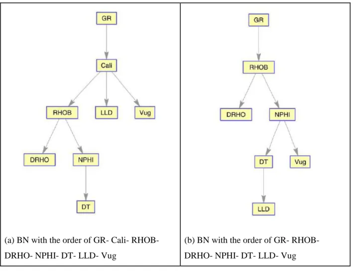
Like understanding causal relationships for fracture identification, sequential procedure
of constructing BN is used for vug detection too (Fig. 9). The first BN is constructed by the order
of: GR- Cali- RHOB- DRHO- NPHI- DT- LLD- Vug
(a) BN with the order of GR- Cali- RHOB- DRHO- NPHI- DT- LLD- Vug
(b) BN with the order of GR- RHOB- DRHO- NPHI- DT- LLD- Vug
4 5 6 7 8 9 10 11 12 13 14 15 16 17 18 19 20 21 22 23 24 25 26 27 28 29 30 31 32 33 34 35 36 37 38 39 40 41 42 43 44 45 46 47 48 49 50 51 52 53 54 55 56 57 58 59
(c) BN with the order of GR- RHOB- DRHO- DT- LLD- Vug
(d) BN with the order of GR- RHOB- DRHO- LLD- Vug
(e) BN with the order of GR- DRHO- LLD- Vug
4 5 6 7 8 9 10 11 12 13 14 15 16 17 18 19 20 21 22 23 24 25 26 27 28 29 30 31 32 33 34 35 36 37 38 39 40 41 42 43 44 45 46 47 48 49 50 51 52 53 54 55 56 57 58 59 60 61
Fig. 9. Bayesian Networks in Sarvak Formation of F3.
Calliper log is the most important feature for vug detection (Fig. 9 (a)); NPHI, DT,
RHOB and GR are other important features in order.
6.4. Causal Relationships for Net Pay Determination
Determining productive zones is a very critical stage in static reservoir modelling.
Petrophysical net pay determination is usually done by cut-off method. Some of utilized features
in literature are included in Table 5.
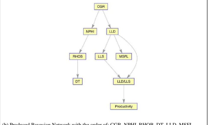
For net pay detection, production rate, derived from production test is utilized as criteria
of productivity:
(a) Productivity of 1 means that production rate is less than 1000 barrel oil per
day [ ]
(b) Productivity of 2 means that production rate is between 1000
[ ] and 1500 barrel daily [ ]
(c) Productivity of 3 means that production rate is more than 1500 barrel per day
[ ] 4 5 6 7 8 9 10 11 12 13 14 15 16 17 18 19 20 21 22 23 24 25 26 27 28 29 30 31 32 33 34 35 36 37 38 39 40 41 42 43 44 45 46 47 48 49 50 51 52 53 54 55 56 57 58 59
Like Fig. 5 (a) and (b), cross plots of F1 are plotted, and correlation coefficients are
calculated. Due to productivity, LLD/LLS, RHOB, LLD and DT are the most effective features
for modelling well test results. Based on dependency criterion (Fig. 10 (b)), LLD/LLS is the
most important feature likewise. LLD and LLS are in the second stage of importance.
(a) Correlation Coefficients and histograms
4 5 6 7 8 9 10 11 12 13 14 15 16 17 18 19 20 21 22 23 24 25 26 27 28 29 30 31 32 33 34 35 36 37 38 39 40 41 42 43 44 45 46 47 48 49 50 51 52 53 54 55 56 57 58 59 60 61
(b) Produced Bayesian Network with the order of: CGR, NPHI, RHOB, DT, LLD, MSFL, LLS, LLD/LLS and Productivity
Fig. 10. Relationships between features in Sarvak Formation of F1 for net pay detection.
In order to satisfy the second goal of the paper, which is providing results of feature
selection in order to benefit petrophysiscists of, selected features for reservoir characterization
are summarized in Table 6. 1st stage features are those features that have high priority due to both criteria; 2nd stage features are those effective features that do not have the same importance as 1st stage features. For fracture detection, there is another column named 3rd stage features that are not as important as 2nd stage features. It is worthy to mention that bulk density (RHOB) is the most frequent feature in this table; therefore, the most important log for reservoir
characterization. 4 5 6 7 8 9 10 11 12 13 14 15 16 17 18 19 20 21 22 23 24 25 26 27 28 29 30 31 32 33 34 35 36 37 38 39 40 41 42 43 44 45 46 47 48 49 50 51 52 53 54 55 56 57 58 59
Tables 3, 4 and 5 are included in the current work in order to validate obtained results,
i.e. proposed input features for reservoir study, Table 6. Comparing the current (Table 6) and
previous works (Tables 3, 4 and 5) reveals that selected features (Table 6) are reasonable for
porosity, permeability, fracture, vug and net pay studies; furthermore, combining BN and
correlation coefficient is a successful way for feature extraction in reservoir characterisation.
7. Conclusion
Although correlation coefficient is a very useful and easy to use criterion to find and
quantify mutual relationships between different variables, there are some pitfalls when using it.
In this work, Bayesian Network is introduced as a complementary means (not an alternative) to
find out dependency relations; therefore, finding causal relationships and feature selection in
reservoir characterization. The results showed that RHOB, DT and NPHI are the most important
features for porosity estimation; whereas Porosity and RHOB are the most effective variables on
estimating permeability. DT and SGR are introduced as very effective features for fracture
identification, and for vug detection, NPHI, DT, RHOB and Calliper are recommended. Finally,
resistivity logs of LLD/LLS and LLD have been proved to be the most valuable features for net
pay detection.
Acknowledgment
The authors wish to acknowledge Exploration Directorate of National Iranian Oil
Company (NIOC), for permission to publish scientific results. Also, special thanks to Mr.
Meisam Akbari Zare, a professional mountain climber for sharing his nice photo of Damavand
Mountain with us. Finally, many thanks to Dr. Abdullah M. Al-Amri and Dr. Jassim M. Thabit,
4 5 6 7 8 9 10 11 12 13 14 15 16 17 18 19 20 21 22 23 24 25 26 27 28 29 30 31 32 33 34 35 36 37 38 39 40 41 42 43 44 45 46 47 48 49 50 51 52 53 54 55 56 57 58 59 60 61
editor-in-chief and reviewer of Arabian Journal of Geosciences for their comments and review on submitted manuscript.
References
Abdollahzadeh, A. et al., 2011. Estimation of Distribution Algorithms Applied to History Matching, SPE Reservoir Simulation Symposium. Society of Petroleum Engineers, The Woodlands, Texas, USA.
Al-Ameri, T.K., Al-Khafaji, A.J. and Zumberge, J., 2009. Petroleum system analysis of the Mishrif reservoir in the Ratawi, Zubair, North and South Rumaila oil fields, southern Iraq. GeoArabia, 14(4): 91-108.
Al-yami, A.S. and Schubert, J., 2012. Underbalanced Drilling Expert System Development, SPE Western Regional Meeting. Society of Petroleum Engineers, Bakersfield, California, USA.
Al-Yami, A.S., Schubert, J., Medina-Cetina, Z. and Yu, O.-Y., 2010. Drilling Expert System for the Optimal Design and Execution of Successful Cementing Practices, IADC/SPE Asia Pacific Drilling Technology Conference and Exhibition. 2010, IADC/SPE Asia Pacific Drilling Technology Conference and Exhibition, Ho Chi Minh City, Vietnam.
Al-yami, A.S., Schubert, J.J. and Beck, F.E., 2011. Expert System for the Optimal Design and Execution of Successful Completion Practices Using Artificial Bayesian Intelligence, Brasil Offshore. Society of Petroleum Engineers, Macaé, Brazil.
Asgari-Nezhad, Y., Sherkati, S. and Tokhmechi, B., 2012. Differentiation between vugular porosity and other kinds of porosities using signal processing operators. Exploration & Production Oil & Gas, 96: 91-98.
Asgarinezhad, Y., Tokhmechi, B., Roohani, A.K., Sherkati, S. and Jamali, A., 2011. Ranking of well logs in identification of vugs, 29rd Symposium on Geosciences. Geological survey of Iran, Tehran.
Bleiholder, J. and Naumann, F., 2008. Data Fusion. ACM Computing Surveys, 41(1): 1-41. Bobko, P., 2001. A Review of the Correlation Coefficient and Its Properties, Correlation and
Regression. SAGE.
Cooper, G.F. and Herskovits, E., 1992. A Bayesian method for the induction of probabilistic networks from data. Machine Learning, 9(4): 309-347.
Doguc, O. and Ramirez-Marquez, J.E., 2009. A generic method for estimating system reliability using Bayesian networks. Reliability Engineering & System Safety, 94(2): 542-550. Duda, R.O., Hart, P.E. and Stork, D.G., 2000. Pattern Classification. Wiley India Pvt. Ltd. Fethi, E., Nabil, M., Salim El-Djoudi, M. and Peter Andrew, H., 2010. How to integrate Wireline
Formation Tester, Logs, Core and Well Test Data to get Hydraulic Flow Unit
4 5 6 7 8 9 10 11 12 13 14 15 16 17 18 19 20 21 22 23 24 25 26 27 28 29 30 31 32 33 34 35 36 37 38 39 40 41 42 43 44 45 46 47 48 49 50 51 52 53 54 55 56 57 58 59
Permeability, SPE Production and Operations Conference and Exhibition. Society of Petroleum Engineers, Tunis, Tunisia.
Ghoraishy, S.M., Liang, J.T., Green, D.W. and Liang, H.C., 2008. Application of Bayesian networks for predicting the performance of gel-treated wells in the arbuckle formation, Kansas. 16th SPE/DOE Improved Oil Recovery Symposium 2008 - "IOR: Now More Than Ever.", Tulsa, OK, pp. 702-708.
Helle, H.B., Bhatt, A. and Ursin, B., 2001. Porosity and permeability prediction from wireline logs using artificial neural networks: a North Sea case study. Geophysical Prospecting, 49(4): 431-444.
Hermann, R. et al., 2011. Water Production Surveillance Workflow using Neural Network and Bayesian Network Technology: A Case Study of Bongkot North Field, Thailand, International Petroleum Technology Conference. International Petroleum Technology Conference, Bangkok, Thailand.
Ibrahim Sami, N. and Adel, M., 2010. Permeability Prediction from Wireline Well Logs Using Fuzzy Logic and Discriminant Analysis, SPE Asia Pacific Oil and Gas Conference and Exhibition. Society of Petroleum Engineers, Brisbane, Queensland, Australia.
Ja'Fari, A., Kadkhodaie-Ilkhchi, A., Sharghi, Y. and Ghanavati, K., 2012. Fracture density estimation from petrophysical log data using the adaptive neuro-fuzzy inference system. Journal of Geophysics and Engineering, 9(1): 105-114.
Jalali Lichaei, M. and Nabi Bidhendi, M., 2006. Comparison between Multiple Linear Regression and Artificial Neural Networks for Porosity and Permeability Estimation. Geosciences Scientific Quarterly Journal, 61: 140-149.
Jensen, J.L. and Menke, J.Y., 2006. Some Statistical Issues in Selecting Porosity Cutoffs for Estimating Net Pay. PetroPhysics, 47(4): 315–320.
Kannan, P., 2006. Bayesian Networks: Application in safety instrumentation and risk reduction. Hydrocarbon Asia, 16(6).
Khaz'ali, A.R., Farahani, F.J. and Ahmadabadi, M.N., 2011. Bayesian network - A new
probabilistic method for petroleum reservoir production prediction and history matching. Petroleum Science and Technology, 29(7): 745-757.
Khor, K.C., Ting, C.Y. and Amnuaisuk, S.P., 2009. From feature selection to building of Bayesian classifiers: A network intrusion detection perspective. American Journal of Applied Sciences, 6(11): 1949-1960.
Lauría, E., 2008. An Information-Geometric Approach to Learning Bayesian Network Topologies from Data. In: D. Holmes and L. Jain (Editors), Innovations in Bayesian Networks. Studies in Computational Intelligence. Springer Berlin / Heidelberg, pp. 187-217.
Lee Rodgers, J. and Nicewander, W.A., 1988. Thirteen ways to look at the correlation coefficient. The American Statistician, 42(1): 59-66.
Mahbaz, S., Sardar, H., Namjouyan, M. and Mirzaahmadian, Y., 2011. Optimization of reservoir cut-off parameters: a case study in SW Iran. Petroleum Geoscience, 17(4): 355-363.
4 5 6 7 8 9 10 11 12 13 14 15 16 17 18 19 20 21 22 23 24 25 26 27 28 29 30 31 32 33 34 35 36 37 38 39 40 41 42 43 44 45 46 47 48 49 50 51 52 53 54 55 56 57 58 59 60 61
Mansure, A.J., Whitlow, G.L., Corser, G.P., Harmse, J. and Wallace, R.D., 1999. A Probabilistic Reasoning Tool for Circulation Monitoring Based on Flow Measurements, SPE Annual Technical Conference and Exhibition. Society of Petroleum Engineers, Houston, Texas. Martinelli, G., Eidsvik, J., Hauge, R. and Førland, M.D., 2011. Bayesian networks for prospect
analysis in the North Sea. AAPG Bulletin, 95(8): 1423-1442.
Martinelli, G., Eidsvik, J., Sinding-Larsen, R., Rekstad, S. and Mukerji, T., 2013. Building Bayesian networks from basin-modelling scenarios for improved geological decision making. Petroleum Geoscience, 19(3): 289-304.
Masoudi, P., Hourfar, F. and Mazaheri Torei, A., 2011a. An Improvement in Estimating Petrophysical Parameters by Utilizing Normalizing Mapping on Inputs of Artificial Neural Networks, 8th Iranian Student Mining Engineering Conference, Tehran, Iran, pp. 1-8.
Masoudi, P., Tokhmechi, B., Ansari Jafari, M., Zamanzadeh, S.M. and Sherkati, S., 2012a. Application of Bayesian in determining productive zones by well log data in oil wells. Journal of Petroleum Science and Engineering, 94–95(0): 47-54.
Masoudi, P., Tokhmechi, B., Bashari, A. and Jafari, M.A., 2012b. Identifying productive zones of the Sarvak formation by integrating outputs of different classification methods. Journal of Geophysics and Engineering, 9(3): 282-290.
Masoudi, P., Tokhmechi, B., Jafari, M.A. and Moshiri, B., 2012c. Application of Fuzzy
Classifier Fusion in Determining Productive Zones in Oil Wells. Energy Exploration and Exploitation, 30(3): 403-415.
Masoudi, P., Tokhmechi, B., Zahedi, A. and Jafari, M.A., 2011b. Developing a Method for Identification of Net Zones Using Log Data and Diffusivity Equation. Journal of Mining and Environment, 2(1): 53-60.
Mehri, M., 2010. Optimization of Permeability Estimation by Using Hydraulic Flow Units in Hydrocarbon Reservoirs, University of Tehran, 160 pp.
Niedermayer, D., 2008. An introduction to Bayesian networks and their contemporary
applications. In: D.E. Holmes and L.C. Jain (Editors), Innovations in Bayesian Networks, Theory and Applications. Studies in computational intelligence. Springer, Berlin, pp. 117-130.
Olofsson, P., 2011. Probability, statistics, and stochastic processes. Wiley-Interscience. OxfordDictionaries, 2010. "dependence". Oxford Dictionaries. April 2010. Oxford University
Press.
Pearl, J., 1986. Fusion, propagation, and structuring in belief networks. Artificial Intelligence, 29(3): 241-288.
Rajabi, M., Sherkati, S., Bohloli, B. and Tingay, M., 2010. Subsurface fracture analysis and determination of in-situ stress direction using FMI logs: An example from the Santonian carbonates (Ilam Formation) in the Abadan Plain, Iran. Tectonophysics, 492(1–4): 192-200. 4 5 6 7 8 9 10 11 12 13 14 15 16 17 18 19 20 21 22 23 24 25 26 27 28 29 30 31 32 33 34 35 36 37 38 39 40 41 42 43 44 45 46 47 48 49 50 51 52 53 54 55 56 57 58 59
Rajaieyamchee, M.A. and Bratvold, R.B., 2009. Real time decision support in drilling operations using Bayesian Decision Networks. SPE Annual Technical Conference and Exhibition 2009, ATCE 2009, New Orleans, LA, pp. 1517-1533.
Rasheva, S. and Bratvold, R.B., 2011. A new and improved approach for geological dependency evaluation for multiple-prospect exploration. SPE Annual Technical Conference and Exhibition 2011, ATCE 2011, Denver, CO, pp. 3422-3431.
Russo, F. and Ramponi, G., 1994. Fuzzy methods for multisensor data fusion. Instrumentation and Measurement, IEEE Transactions on 43(2): 288-294.
Saemi, M., Ahmadi, M. and Varjani, A.Y., 2007. Design of neural networks using genetic algorithm for the permeability estimation of the reservoir. Journal of Petroleum Science and Engineering, 59(1-2): 97-105.
Shahvar, M.B., Kharrat, R. and Mahdavi, R., 2009. Incorporating Fuzzy Logic and Artificial Neural Networks for Building a Hydraulic Unit-Based Model for Permeability Prediction of a Heterogeneous Carbonate Reservoir, International Petroleum Technology
Conference, Doha, Qatar.
Sherkati, S. and Letouzey, J., 2004. Variation of structural style and basin evolution in the central Zagros (Izeh zone and Dezful Embayment), Iran. Marine and Petroleum Geology, 21(5): 535-554.
Timothy, O.S., Dennis, B., Praveer, K. and Rohit, T., 2008. Mangala Field Permeability
Measurements: Comparison of Core, Wireline, and Well Test Data, SPE Indian Oil and Gas Technical Conference and Exhibition. Society of Petroleum Engineers, Mumbai, India.
Tokhmchi, B., Memarian, H. and Rezaee, M.R., 2010. Estimation of the fracture density in fractured zones using petrophysical logs. Journal of Petroleum Science and Engineering, 72(1–2): 206-213.
Tokhmechi, B., Memarian, H., Rasouli, V., Noubari, H.A. and Moshiri, B., 2009. Fracture detection from water saturation log data using a Fourier–wavelet approach. Journal of Petroleum Science and Engineering, 69(1–2): 129-138.
Van Wees, J.D. et al., 2008. A Bayesian belief network approach for assessing the impact of exploration prospect interdependency: An application to predict gas discoveries in the Netherlands. AAPG Bulletin, 92(10): 1315-1336.
Worthington, P.F., 2010. Net Pay-What Is It? What Does It Do? How Do We Quantify It? How Do We Use It? SPE Reservoir Evaluation & Engineering, 13(5): pp. 812-822.
Zerafat, M.M., ayatollahi, s., Mehranbod, N. and Barzegari, D., 2011. Bayesian Network Analysis as a Tool for Efficient EOR Screening, SPE Enhanced Oil Recovery Conference. Society of Petroleum Engineers, Kuala Lumpur, Malaysia.
Zuo, Y. and Kita, E., 2012. Stock price forecast using Bayesian network. Expert Systems with Applications, 39(8): 6729-6737. 4 5 6 7 8 9 10 11 12 13 14 15 16 17 18 19 20 21 22 23 24 25 26 27 28 29 30 31 32 33 34 35 36 37 38 39 40 41 42 43 44 45 46 47 48 49 50 51 52 53 54 55 56 57 58 59 60 61
a
a
a
a
a
a
1
3
5
Table 1. The table shows what reservoir properties are studied in which field
Porosity Permeability Net Pay Fracture Vug
F1: 6 wells Abadan Plain
F2: 1 well South Dezful
Table 2. Summary of dataset of F1 oil field, available for evaluating causality relationships for assessing
porosity, permeability and net pay zones
Well 1 Well 2 Well 3 Well 4 Well 5 Well 6
No. of Well Test Intervals
3 2 4 1 1 3 1 1 1 1 1 3 Petr o p h y sical W ell L o g s Calliper (CALI) Gamma Rey (GR)
Gamma Ray Contribution from Thorium
and Potassium (CGR)
Sonic Log (DT)
Thermal Neutron Porosity in Selected
Lithology (NPHI)
Bulk Density (RHOB)
Bulk Density Correction (DRHO)
Laterolog Deep Resistivity (LLD)
Laterolog Shallow Resistivity (LLS) Micro-spherically-focused Resistivity
(MSFL)
Photoelectric Factor (PEF)
C o re T ests Porosity Permeability
Table 3. Petrophysical parameters for porosity estimation in various references
Used Parameters for Estimation Source
Po
ro
sity
NPHI, Density, Sonic, Resistivity (Helle et al. 2001)
DT, GR, ILD, ILS, NPHI, RHOB (Jalali Lichaei and Nabi Bidhendi 2006) CGR, DT, LLD, LLS, MSFL, NPHI, RHOB (Masoudi et al. 2011b)
Per m ea b ilit y
NPHI, Density, Sonic, Resistivity (Helle et al. 2001)
Depth, DT, GR, ILD, ILS, RHOB, Sw, Porosity (Jalali Lichaei and Nabi Bidhendi 2006) NMR (Fethi et al. 2010; Timothy et al. 2008) SGR, CGR, RHOB, TNPH (Thermal Neutron Porosity),
Rs (medium resistivity), Rt (deep Resistivity), Rxo (shallow resistivity), DT, VCLAY (clay volume)
(Shahvar et al. 2009)
Saturation, Gamma, Neutron, RHOB, PEF, DT,
Resistivity (Saemi et al. 2007)
Gamma, DT, Nphi, RHOB, LLD/LLS (Ibrahim Sami and Adel 2010) NPHI, RHOB, DT, LLD, SGR, CGR (Mehri 2010)
Table 4. Petrophysical parameters for evaluating secondary porosity
Used Parameters for Identification Source
Fra
ctu
re
Water Saturation, GR (Tokhmechi et al., 2009) Calliper, DT, RHOB, PEF (Tokhmchi et al., 2010) DT, RHOB, NPHI, Resistivity (Ja'Fari et al., 2012)
Vu
g NPHI, DT, GR, Calliper (Asgarinezhad et al., 2011) NPHI, DT, GR, RHOB (Asgari-Nezhad et al., 2012)
Table 5. Petrophysical parameters for net pay determination in various references
Used Parameters for detection Source
Shale Volume, Porosity, Water Saturation (Jensen and Menke 2006; Mahbaz et al. 2011; Worthington 2010) Permeability, Porosity, Viscosity, Compressibility (Masoudi et al. 2011b)
Porosity, Water Saturation, Shale Volume (Masoudi et al. 2012a) Ratio of LLD to LLS and LLD (Masoudi et al. 2012c)
Table 6. Result of feature selection for porosity, permeability, fracture detection, vug detection and net
pay determination due to correlation coefficient and Bayesian Network
1st stage 2nd stage 3rd stage
Porosity RHOB DT NPHI LLD CGR -- Permeability Porosity RHOB LLD NPHI DT -- Fracture DT SGR RHOB PEF CGR Vug NPHI DT RHOB Cali -- -- Net Pay LLD/LLS LLD LLS RHOB --