HAL Id: hal-02430592
https://hal.sorbonne-universite.fr/hal-02430592
Submitted on 7 Jan 2020
HAL is a multi-disciplinary open access
archive for the deposit and dissemination of
sci-entific research documents, whether they are
pub-lished or not. The documents may come from
teaching and research institutions in France or
abroad, or from public or private research centers.
L’archive ouverte pluridisciplinaire HAL, est
destinée au dépôt et à la diffusion de documents
scientifiques de niveau recherche, publiés ou non,
émanant des établissements d’enseignement et de
recherche français ou étrangers, des laboratoires
publics ou privés.
Fluxes in Oxygen Minimum Zone Regions
Rainer Kiko, Helena Hauss
To cite this version:
Rainer Kiko, Helena Hauss. On the Estimation of Zooplankton-Mediated Active Fluxes in
Oxy-gen Minimum Zone Regions.
Frontiers in Marine Science, Frontiers Media, 2019, 6, pp.741.
ORIGINAL RESEARCH published: 06 December 2019 doi: 10.3389/fmars.2019.00741
Edited by: Sanjeev Kumar, Physical Research Laboratory, India Reviewed by: John Patrick Dunne, Geophysical Fluid Dynamics Laboratory (GFDL), United States Jyothibabu Retnamma, Council of Scientific and Industrial Research, India *Correspondence: Rainer Kiko rainer.kiko@obs-vlfr.fr
Specialty section: This article was submitted to Marine Biogeochemistry, a section of the journal Frontiers in Marine Science Received: 20 May 2019 Accepted: 14 November 2019 Published: 06 December 2019 Citation: Kiko R and Hauss H (2019) On the Estimation of Zooplankton-Mediated Active Fluxes in Oxygen Minimum Zone Regions. Front. Mar. Sci. 6:741. doi: 10.3389/fmars.2019.00741
On the Estimation of
Zooplankton-Mediated Active Fluxes
in Oxygen Minimum Zone Regions
Rainer Kiko1,2* and Helena Hauss11Marine Ecology, GEOMAR Helmholtz Institute for Ocean Research Kiel, Kiel, Germany,2Laboratoire d’Océanographie de
Villefranche, Sorbonne Université, Villefranche-sur-Mer, France
In the Peruvian upwelling system, the mesopelagic oxygen minimum zone (OMZ) is the main vertically structuring feature of the pelagic habitat. Several zooplankton and nekton species undertake diel vertical migrations (DVMs) into anoxic depths. It has been argued that these migrations contribute substantially to the oxygen consumption and release of dissolved compounds (in particular ammonium) in subsurface waters. However, metabolic suppression as a response to low ambient oxygen partial pressure (pO2) has not been accounted for in these estimates. Here, we present estimates of
zooplankton- and nekton-mediated oxygen consumption and ammonium release based on vertically stratified net hauls (day/night, upper 1,000 m). Samples were scanned, followed by image analysis and size-/taxon-specific estimation of metabolic rates of all identified organisms as a function of their biomass as well as ambient temperature and pO2. The main crustacean migrants were euphausiids (mainly E. mucronata) on
offshore stations and the commercially exploited squat lobster Pleuroncodes monodon on the upper shelf, where it often undertakes migration to the seafloor during the day. Correction for metabolic suppression results in a substantial reduction of both respiration and ammonium excretion within the OMZ core. Ignoring this mechanism leads to a 10-fold higher estimate of DVM-mediated active export of carbon by respiration to below 100 m depth at deep-water stations. The DVM-mediated release of ammonium by euphausiids into the 200–400 m depth layer ranges between 0 and 36.81 µmol NH4m−2
d−1, which is insufficient to balance published estimates of ammonium uptake rates due to anammox. It seems critical to account for the modulation of zooplankton metabolic activity at low oxygen in order to correctly represent the contribution of migrating species to the biological pump.
Keywords: zooplankton, Humboldt current, export flux, krill, biological carbon pump
1. INTRODUCTION
Zooplankton organisms occupy an important role in pelagic ecosystems as they provide the link between primary and tertiary trophic levels and to a large extent shapes elemental cycles. Depth-integrated mesozooplankton carbon ingestion and respiration of primary production in the global open ocean is estimated at 34–63 and 17–32%, respectively (Hernández-León and Ikeda, 2005). Zooplankton organisms feed on all kinds of small particulate matter (e.g., phytoplankton,
detritus, other zooplankton) and egested fecal pellets contribute substantially to the passive sinking flux out of the surface layer.
The diel vertical migration (DVM) of zooplankton and micronekton is the largest concerted movement of animal biomass on earth. In the most common form, zooplankton organisms actively feed in the productive euphotic zone during the night and migrate down to a few hundred meters depth during the day to mainly hide from visual predation (Lampert, 1989). These DVMs result in the active export of organic and inorganic matter from the surface layer as zooplankton organisms excrete, defecate, respire and are preyed upon at depth (e.g., Longhurst et al., 1990). The daytime depth is strongly dependent on water transparency and is deepest in the oligotrophic blue ocean. In the Peruvian upwelling system, one of the most productive regions on the planet, microbial degradation of sinking organic matter (Kalvelage et al., 2015) and respiration by metazoans, in concert with sluggish ventilation (Czeschel et al., 2011) have led to the formation of a permanent oxygen minimum zone (OMZ) with often virtually anoxic oxygen concentrations in its core (e.g.,Revsbech et al., 2009). The core of this midwater OMZ coincides with the daytime depth of many DVM species as indicated by large scale analysis of acoustic backscatter data (Bianchi et al., 2013, 2014). The upper oxycline, which is located directly below the mixed layer, is considered the single most important vertically structuring feature of the pelagic habitat in the Humboldt Current Ecosystem (Chavez and Messié, 2009; Bertrand et al., 2010). At the same time, oxygen levels play an essential role in nutrient cycling. Under anoxic conditions, N loss processes (denitrification and anammox,Lam et al., 2009) result in a nitrogen deficit in the upwelling regions.
Bianchi and Mislan (2016) suggested that zooplankton DVM is a major contributor to providing dissolved ammonium to the OMZ by excretion at the daytime depth. However, they did not account for changes in zooplankton metabolism at low oxygen levels.
Zooplankton organisms ultimately rely on aerobic respiration. They developed different, species-specific hypoxia tolerance thresholds (Childress and Seibel, 1998) and some tolerate anoxia for prolonged periods of time. OMZs therefore shape the distribution of zooplankton within the pelagic ecosystem (e.g.,
Saltzman and Wishner, 1997; Wishner et al., 1998; Auel and Verheye, 2007). Off Peru, only few metazoan species are able to tolerate anoxic conditions in the OMZ core. These include the endemic krill species Euphausia mucronata (Kiko et al., 2016) and the squat lobster Pleuroncodes monodon (Kiko et al., 2015). They achieve this by downregulation of their aerobic metabolism. As they “hold their breath,” oxygen consumption is not measurable, but also ammonium excretion is substantially reduced (Kiko et al., 2015, 2016). Up to now, this metabolic suppression has not been accounted for in estimations of DVM-mediated fluxes.
Here, we examine the vertical distribution and migration of zooplankton in the upper 1,000 m off Peru. We develop a new method to include the impact of low oxygen levels on metabolic function to better constrain zooplankton impacts on the carbon, nitrogen and oxygen budget of the area.
2. MATERIALS AND METHODS
2.1. Field Sampling
Data and samples were collected during RV Meteor cruise 93 to the Peruvian upwelling region in February and March 2013 (2013/02/06 to 2013/03/10, Callao/Peru to Cristobal/Panama), At the time of the cruise, southeasterly winds prevailed (1 − 9 m s−1,Thomsen et al., 2016), resulting in nutrient upwelling
typical of austral summer conditions. At five stations, we took depth-specific mesozooplankton samples conducting 10 vertical hauls (1 m s−1) with a Hydrobios MultiNet Maxi (0.50 m2
mouth opening, 333 µm mesh size, 9 nets). During each station occupation, a day haul and a night haul were obtained within 24 h and in very close proximity (average distance 0.15 km, range 0–0.7 km) to each other, representing a pair of day-night hauls for the assessment of diel vertical migration patterns. Sampling was avoided during local dusk or dawn ±1 h. The day hauls were brought on deck ±5 h of local solar noon, whereas the night hauls were brought on deck ±4 h of local midnight (see Figure 1 for sampling locations and Table 1 for further location and time information for each haul used). Sampling depths were 1,000–600, 600–400, 400–200, 200–100, 100–50, 50–30, 30–20, 20–10, and 10–0 m depth when water depth was >1,000 m. Otherwise, a finer depth resolution within these general depth steps was established. Temperature, salinity and oxygen concentration from RV Meteor cruise 93 were measured by the Physical Oceanography department at the GEOMAR Helmholtz Centre for Ocean Research Kiel and are published byKrahmann (2015). In short, a Seabird SBE 9-plus CTD on a 24-niskin rosette was deployed directly before or after the net haul. The CTD carried duplicate temperature, salinity and oxygen (optode) probes. Oxygen from the optodes was calibrated by a combination of Winkler titration (Grasshoff et al., 2009) and STOX sensor measurements (Revsbech et al., 2009). Zooplankton samples were formaldehyde-fixed on board and brought to the GEOMAR laboratory.
2.2. Zooplankton Imaging and Biomass
Calculation
In the laboratory, each sample was size-fractionated (small: 333– 500 µm, medium: 500–1000 µm and large: > 1, 000 µm). For the small and medium fraction, subsamples with about 1,000 zooplankton items per subsample were generated using a Motoda-Splitter, whereas the entire large fraction was used for further analysis. The plankton items contained in each fraction were distributed and separated on a 20*30 cm glass tray and the glass tray scanned using an Epson perfection V750 pro flatbed scanner. Scans were 8bit grayscale, 2,400 dpi images (tagged image file format; *.tif). Object segmentation was conducted using Zooprocess (Gorsky et al., 2010) and taxonomic units were assigned automatically using Plankton Identifier or the prediction options in EcoTaxa (Picheral et al., 2019). Assignments were thereafter corrected manually on the EcoTaxa platform. Analysis of the biomass-size spectrum showed that organisms with an equivalent spherical diameter of 12.41 mm were not quantitatively sampled. Therefore, this value was chosen as a digital cut-off in our analysis, meaning that all objects larger then
Kiko and Hauss Zooplankton-Mediated Fluxes in OMZs
FIGURE 1 | Map of the Eastern Tropical South Pacific (left) with a red rectangle indicating study area (right) and red dots indicating sites (S1–S5). At each of the five sampling sites, a pair of day and night hauls were obtained.
TABLE 1 | Metadata for each pair of hauls used in this publication.
Pair ID (–) Haul ID (–) Date (–) Time (UTC) Lat. (◦) Lon. (◦) Noon (UTC) Delta to noon (h) Category (–) In pair dist. (km) Dist. to coast (km) Max. depth sampled (m) s1 mn25 2013-03-02 22:22 −12.254 −77.152 17:20 05:01 Day 0.11 12.8 70 s1 mn26 2013-03-03 02:29 −12.254 −77.153 17:20 09:08 Night 0.11 12.8 70 s2 mn02 2013-02-10 21:10 −12.38 −77.191 17:22 03:47 Day 0.0 24.2 125 s2 mn03 2013-02-11 02:58 −12.38 −77.191 17:22 09:35 Night 0.0 24.2 125 s3 mn20 2013-02-24 21:35 −12.377 −77.388 17:22 04:12 Day 0.0 41.6 210 s3 mn19 2013-02-24 07:58 −12.377 −77.388 17:22 14:35 Night 0.0 41.6 210 s4 mn05 2013-02-11 20:58 −12.639 −77.531 17:24 03:33 Day 0.69 71.0 1000 s4 mn04 2013-02-11 09:30 −12.633 −77.537 17:24 16:05 Night 0.69 71.0 1000 s5 mn14 2013-02-20 18:47 −12.668 −77.821 17:24 01:22 Day 0.0 98.5 1000 s5 mn13 2013-02-20 08:05 −12.668 −77.821 17:25 14:39 Night 0.0 98.5 1000
this size were not further considered when calculating biomass or metabolic rates. Likewise, the small fraction (333–500 µm) was not included, as preliminary analysis showed almost no DVM-activity into the OMZ in this size fraction. Taxon-specific area-to-drymass conversion factors for subtropical zooplankton (Lehette and Hernández-León, 2009) were used to calculate the dryweight of each specimen according to dw = a ∗ areab. Likewise,
taxon-specific drymass to C conversion factors (Kiørboe, 2013) were used to calculate the C content of each zooplankton organism scanned. Taxonomic units and biomass conversion factors used are listed in Table 2. Abundance and biomass estimates are lower bounds, as some organisms sticked together, produced an undiscernable mass with detritus or in case of gelatinous organisms did not produce a clearly identifiable image due to the low contrast of the tissue. Such individuals were not included in the respective calculations.
The following categories cannot be discerned in the preserved net samples, as many of their members are either damaged by the net or the fixation and therefore do not yield quantifiable images: thaliacea, cnidaria other then calycophoran siphonophores, ctenophores, all rhizaria.
We consider the following categories to be well-conserved and constrain our analyses on these: crustacea, chaetognatha, calycophoran siphonophores, annelida, and mollusca. Fish are also well-conserved, but not included in the literature on zooplankton individual biomass estimates or metabolic rates (Lehette and Hernández-León, 2009; Kiørboe, 2013; Ikeda, 2014) we use.
2.3. Estimation of Physiological
Rates—Respiration
Taxon-specific equations for biomass and temperature dependence of respiration (Ikeda, 2014) were applied to calculate the depth-specific respiration rate of each scanned crustacean specimen. A detailed description on the experimental procedure to estimate these rates is given in Ikeda (1985). The average temperature for the sampled depth layer was obtained from the concomitant CTD deployments. We applied a correction for the oxygen-dependence of respiration if the mean oxygen level for a given net was below the critical oxygen partial pressure pcrit of Euphausia mucronata and Pleuroncodes monodon (Kiko
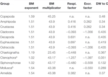
TABLE 2 | Conversion factors and functions used in this publication. Group BM exponent BM multiplicator Respi. factor Excr. factor DW to C
Copepoda 1.59 45.25 n.a. n.a. 0.48 Amphipoda 1.51 43.9 0.416 0.262 0.34 Crustacea 1.51 43.9 0.416 0.262 0.34 Cladocera 1.51 43.9 −0.393 −1.356 0.435 Decapoda 1.51 43.9 0.631 n.a. 0.435 Euphausiacea 1.51 43.9 0.697 n.a. 0.419 Ostracoda 1.51 43.9 −0.393 −1.356 0.435 Chaetognatha 1.19 23.45 −0.448 n.a. 0.367 Ctenophoraa 1.02 43.17 −1.257 −1.397 0.051 Siphonophorae 1.02 43.17 −0.480 −0.558 0.132 Molluscab 1.54 43.38 n.a. −0.550 0.289 Annelida 1.54 43.38 0.382 n.a. 0.37
aFormula for siphonophores was used as no specific formula is given inLehette and
Hernández-León (2009).
bFormula for general mesozooplankton was used as no specific formula is given inLehette
and Hernández-León (2009). Biomass was calculated as biomass = BMmultiplicator ∗ areaBMexponent. Respi. factor and Excr. factor fromIkeda (2014). DW to C conversion factors fromKiørboe (2013). n.a., not applicable.
regulation of oxygen uptake fails, resulting in a drastic metabolic reduction (Childress and Seibel, 1998). As we only have data on the pcrit of these two species from the Peruvian upwelling,
we use the mean of these values (0.6 kPa) as a general pcrit for
crustaceans in the region. These pcrit values were obtained at
13◦C and in order to calculate corrected respiration rates we
need to extrapolate the pcrit to the environmental temperatures
observed. For this, we use Equation (1) byDeutsch et al. (2015):
8 =A0Bn pO2
exp(−E0/kBT)
(1) where 8 is the metabolic index as defined by Deutsch et al. (2015), A0is the ratio of rate coefficients for oxygen supply and
metabolic rate, B is body mass, n is the difference between the allometric scalings of respiratory efficacy and resting metabolic demand, E0is the temperature dependence of resting metabolic
demand and kB is the Boltzmann constant. For further details
regarding this calculation please consultDeutsch et al. (2015). If pO2=pcrit, 8 becomes 1. It follows that the pcritx measured
at temperature x (Tx) and the pcritz measured at temperature z
(Tz) relate to each other in the following way: pcritx
exp(−E0/kBTx)
= pcritz exp(−E0/kBTz)
(2)
If we know pcritz and Tz, we can solve this equation to yield pcritx
at the required target temperature Tx:
pcritx = pcritz ∗ exp((−E0/kBTx) − (−E0/kBTz)) (3)
We use an E0of 0.55, which is the mean of values published for
crustaceans inDeutsch et al. (2015). The E0values provided by
Deutsch et al. (2015) range from 0.36 (Sergestes tenuiremis) to
0.74 (Atlantic rock crab). We assume a linear decrease of the respiration rate from the pcrit to zero, as we have observed that
both crustaceans investigated can tolerate zero oxygen levels and do respire all oxygen if maintained in a closed bottle. Hence, we assume a constant respiration rate for oxygen levels above the extrapolated pcrit (calculated according toIkeda, 2014) and
a linear decrease from pcrit to zero pO2. Figure 2 delineates the
general strategy of this approach. To convert oxygen respiration to carbon release, we use a respiratory quotient of 0.97 (Steinberg and Landry, 2017).
2.4. Estimation of Physiological
Rates—Ammonium Excretion
Ammonium excretion at different oxygen levels was calculated using a reevaluation of the data by Kiko et al. (2016)of rates measured at 13◦C and different oxygen levels for E. mucronata.
Excrstd=a ∗ pO2b+c (4)
with a = 1.275, b = 0.363, and c = 1.0e-10. This yields the excretion rate for 1 g DW of a 0.1 g DW standard individual in µmol h−1g−1. Division by 10 yields the rate for 0.1 g DW of
the 0.1 g DW standard individual in µmol h−1, so essentially the
individual excretion rate.
An allometric weight adjustment according toMoloney and Field (1989)was applied using:
Excr = Excrstd∗((0.1/x)0.25) (5)
with x being the biomass of the individual in g DW. This yields the excretion rate of 0.1 g DW of an organism with biomass x in µmol h−1. Multiplication of this rate with the biomass x
(in g DW) divided by 0.1 g DW (biomass factor, indicates how much heavier or lighter then 0.1 the individual is) yields the excretion rate of the individual with biomass x in µmol h−1.
To scale the rates to the measured in situ temperature, another adjustment was applied using a Q10 of 2. For comparison,
ammonium excretion rates were also calculated according to
Ikeda (2014), which includes an adjustment for temperature, but not for oxygen. At a pO2of 24 kPa, both calculation methods yield
almost identical results (e.g., seeKiko et al., 2016).
2.5. Calculation of Day-Night Biomass
Differences and Active Fluxes
Migratory fluxes from the surface layer to below 100 m depth were calculated as the day-night difference of the integrated biomass at 100–1,000 m depth (or the bottom) to avoid artifacts due to sampling net avoidance in the surface layer at daytime (Ianson et al., 2004). A residence time at depth of 12 h was assumed to calculate metabolic rate related fluxes.
3. RESULTS
3.1. Environmental Conditions
Sea surface temperature (SST) increased from the shelf stations to the offshore stations, with 17.6◦C at the innermost and 20.5◦C
Kiko and Hauss Zooplankton-Mediated Fluxes in OMZs
FIGURE 2 | Schematic of the respiration rate correction for environmental partial pressures below the pcrit. The example calculations are conducted for Euphausiacea
and the transparent dots in the figure indicate individual respiration rate measurements of E. mucronata fromKiko et al. (2016).
FIGURE 3 | Vertical profiles of observed pO2(blue), temperature (red), and pcrit(black) calculated after Equation (3). From left to right: S5, S4, S3, S2, S1 horizontal
gray lines denote sampling intervals of the multinet.
thermo- and oxycline depths decreased from shelf to offshore. The oxygen concentration dropped to < 5 µmol O2 kg−1
at 11, 22, 39, 33, and 42 m depth, respectively, at the five stations (from shelf to offshore). In the OMZ core (between ∼100 and 400 m depth), oxygen content was frequently < 0.5 µmol O2 kg−1 and often reached the detection limit of
the optode. At the two deep stations, an increase in oxygen levels at the base of the OMZ was observed from around 450 m depth, with values higher than 5 µmol O2 kg−1
at 520 and 527 m, respectively. The depth where the observed pO2 fell below the temperature-dependent pcrit value
calculated according to Equation (3) for crustaceans decreased
continuously from nearshore to offshore (11 m at s1 and 42 m at s2; Figure 3).
3.2. Night- and Daytime Biomass
Distribution Along the Sampled Transect
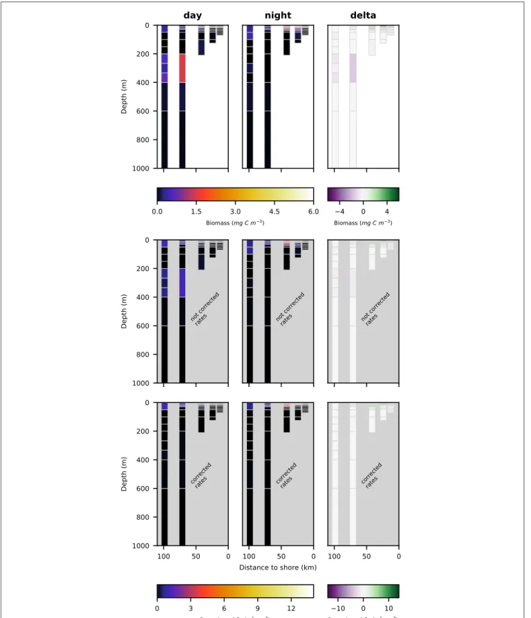
Night- and daytime biomass distribution along the sampled transect is shown for the entire well-preserved zooplankton in Figure 4, top row, for minor groups of well-preserved zooplankton (amphipoda, ostracoda, siphonophora, mollusca, chaetognatha, annelida; abbreviated as MG) in Figure 4, middle row, for decapoda, which were strongly dominated by Pleuroncodes monodon in Figure 4, bottom row and separately
FIGURE 4 | Vertical distribution of zooplankton biomass (mg C m−3) along the transect at day (left panels), night (middle panels), and the difference of the two (right
Kiko and Hauss Zooplankton-Mediated Fluxes in OMZs
FIGURE 5 | Vertical distribution of total crustacean biomass (top row; mg C m−3), not corrected respiration rates (middle row; µmol O
2h−1m−3) and corrected
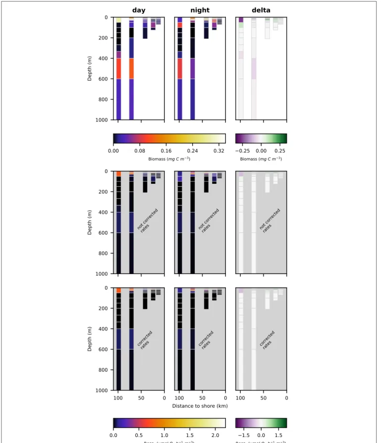
FIGURE 6 | Vertical distribution of copepoda biomass (top row; mg C m−3), not corrected respiration rates (middle row; µmol O
2h−1m−3) and corrected respiration
Kiko and Hauss Zooplankton-Mediated Fluxes in OMZs
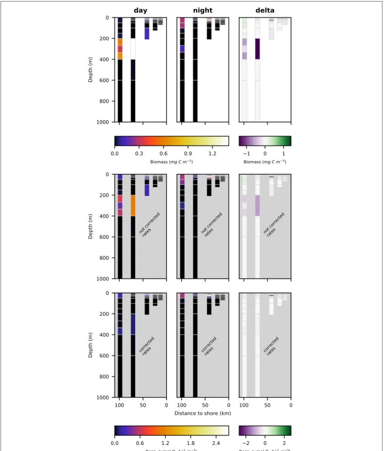
FIGURE 7 | Vertical distribution of euphausiacea biomass (top row; mg C m−3), not corrected respiration rates (middle row; µmol O
2h−1m−3) and corrected
TABLE 3 | Integrated biomass and respiration rates.
Category Parameter Unit s5 s4 s3 s2 s1
Copepod Biomass C night mg C m−2 438.1 310.4 148.6 153.9 13.1
Copepoda Biomass C day mg C m−2 621.8 616.3 44.8 64.2 12.3
Euphausiacea Biomass C night mg C m−2 452.0 15.8 192.1 0.5 11.0
Euphausiacea Biomass C day mg C m−2 1,322.1 3,657.6 201.4 0.1 4.2
Decapoda Biomass C night mg C m−2 33.8 104.0 132.0 1,041.2 9.6
Decapoda Biomass C day mg C m−2 14.1 111.8 19.8 0.2 0.2
Crustacea total Biomass C night mg C m−2 1,617.9 856.1 572.4 2,776.7 36.1
Crustacea total Biomass C day mg C m−2 2,378.1 4,943.0 318.5 123.0 35.8
Minor groups Biomass C night mg C m−2 107.4 143.3 18.6 3.2 27.3
Minor groups Biomass C day mg C m−2 157.5 102.9 67.3 0.6 1.6
Well-preserved total Biomass C night mg C m−2 1,725.4 999.4 591.1 2,779.9 63.3
Well-preserved total Biomass C day mg C m−2 2,535.6 5,045.9 385.8 123.5 37.4
Copepoda Resp. not corrected night mg C m−2d−1 33.2 32.8 19.0 33.9 4.2
Copepoda Resp. not corrected day mg C m−2d−1 62.3 49.6 5.8 11.3 3.2
Euphausiacea Resp. not corrected night mg C m−2d−1 56.9 4.3 39.0 0.2 1.8
Euphausiacea Resp. not corrected day mg C m−2d−1 119.1 232.2 31.5 0.0 0.8
Decapoda Resp. not corrected night mg C m−2d−1 2.7 9.1 23.5 122.5 3.2
Decapoda Resp. not corrected day mg C m−2d−1 3.6 8.5 3.4 0.1 0.1
Crustacea total Resp. not corrected night mg C m−2d−1 143.1 88.0 108.6 425.5 10.0
Crustacea total Resp. not corrected day mg C m−2d−1 219.6 350.2 51.6 19.4 8.8
Minor groups Resp. not corrected night mg C m−2d−1 16.4 17.7 8.4 1.0 10.4
Minor groups Resp. not corrected day mg C m−2d−1 35.0 20.5 21.1 0.2 0.7 Well-preserved total Resp. not corrected night mg C m−2d−1 159.5 105.7 117.0 426.5 20.4
Well-preserved total Resp. not corrected day mg C m−2d−1 254.5 370.7 72.6 19.6 9.5
Copepoda Resp. corrected night mg C m−2d−1 23.7 31.4 17.8 27.3 3.4
Copepoda Resp. corrected day mg C m−2d−1 59.2 46.0 3.1 6.6 1.4
Euphausiacea Resp. corrected night mg C m−2d−1 28.5 3.6 34.9 0.2 0.8
Euphausiacea Resp. corrected day mg C m−2d−1 19.8 23.2 6.3 0.0 0.0
Decapoda Resp. corrected night mg C m−2d−1 1.0 9.1 23.2 107.0 3.0
Decapoda Resp. corrected day mg C m−2d−1 3.6 8.5 1.9 0.1 0.1
Crustacea total Resp. corrected night mg C m−2d−1 94.3 75.4 95.8 378.5 7.5
Crustacea total Resp. corrected day mg C m−2d−1 112.1 109.1 12.9 10.5 4.4
Minor groups Resp. corrected night mg C m−2d−1 0.0 0.0 0.0 0.0 0.0
Minor groups Resp. corrected day mg C m−2d−1 0.0 0.0 0.0 0.0 0.0
Well-preserved total Resp. corrected night mg C m−2d−1 94.3 75.4 95.8 378.5 7.5
Well-preserved total Resp. corrected day mg C m−2d−1 112.1 109.1 12.9 10.5 4.4
for crustacea, copepoda and euphausiacea in Figures 5–7, respectively. Values integrated over the entire water column are shown in Table 3, whereas migratory biomass to below 100 m depth is shown in Table 4.
Total well-preserved zooplankton biomass (Figure 4, top row) was dominated by Pleuroncodes monodon on the shelf and euphausiacea at the offshore stations. In depth layers where these two groups were absent or low in abundance, total well-preserved zooplankton biomass was below 0.1 mg m−3.
Only very little MG zooplankton were found at stations s1 and s2—the two stations closest to the coast (Figure 4, middle row)—and MG zooplankton was dominated by annelida in the surface layers. Highest biomass of the MG group was found at the middle station s3 at daytime, but also stations s4 and s5 featured high MG biomass in the surface layer, dominated
by siphonophora. Siphonophora also generally contributed most to the MG zooplankton biomass. Day-night differences in biomass distribution of the MG zooplankton group showed no clear patterns.
Pleuroncodes monodon was found in high abundance and generated the highest biomass value of 165 mg DW m−3
(62.6 mg C m−3) along the entire transect in surface
waters at station S2 at nighttime. Few further specimens were observed at station s3 in surface waters at nighttime and at station s4 in surface waters at daytime. Virtually no specimens were found in surface waters at daytime at stations s2 and s3.
The biomass of copepoda at station s1 (closest to the shore) was very low, both at day- and at nighttime. The highest biomass of copepoda was found at station s3 in the surface layer at nighttime. Nighttime biomass was also high at stations s2 and
Kiko and Hauss Zooplankton-Mediated Fluxes in OMZs
TABLE 4 | Integrated day-night differences below the 100 m depth level.
Category Parameter Unit s5 s4 s3 s2 s1
Copepod Biomass C mg C m−2 84.3 277.1 1.9 0.0 n.a.
Euphausiacea Biomass C mg C m−2 1,181.4 3,651.0 175.9 0.0 n.a.
Decapoda Biomass C mg C m−2 −32.4 −24.9 8.4 0.0 n.a.
Crustacea total Biomass C mg C m−2 1,005.6 4,097.3 200.3 45.7 n.a.
Minor groups Biomass C mg C m−2 24.4 −29.8 36.7 0.4 n.a.
Well-preserved total Biomass C mg C m−2 1,030.0 4,067.5 237.0 46.1 n.a.
Copepoda Resp. not corrected mg C m−2d−1 0.7 1.9 0.0 0.0 n.a.
Euphausiacea Resp. not corrected mg C m−2d−1 13.8 32.2 3.2 0.0 n.a.
Decapoda Resp. not corrected mg C m−2d−1 −0.3 −0.0 0.1 0.0 n.a.
Crustacea total Resp. not corrected mg C m−2d−1 12.4 37.7 3.8 0.6 n.a.
Minor groups Resp. not corrected mg C m−2d−1 0.8 0.5 1.3 0.0 n.a.
Well-preserved total Resp. not corrected mg C m−2d−1 13.3 38.1 5.1 0.6 n.a.
Copepoda Resp. corrected mg C m−2d−1 0.5 1.6 0.0 0.0 n.a.
Euphausiacea Resp. corrected mg C m−2d−1 1.3 3.1 0.0 0.0 n.a.
Decapoda Resp. corrected mg C m−2d−1 −0.1 −0.0 0.0 0.0 n.a.
Crustacea total Resp. corrected mg C m−2d−1 −0.3 4.8 0.0 0.0 n.a.
Minor groups Resp. corrected mg C m−2d−1 0.0 0.0 0.0 0.0 n.a.
Well-preserved total Resp. corrected mg C m−2d−1 −0.3 4.8 0.0 0.0 n.a.
n.a., not applicable.
s4 in the surface layer. Daytime abundance in the surface layer was low at stations s2 and s3, but comparatively high at stations s4 and s5. A secondary maximum of copepod biomass could be observed at the lower boundary of the OMZ in the two offshore stations s4 and s5 in the 400–600 m depth layer. Day-night differences in biomass distribution of copepoda revealed no clear patterns.
Euphausiacea were almost absent at day and nighttime from the two innermost stations s1 and s2 where water depth was shallower then 200 m. At daytime, euphausiacea biomass was very low in the upper 200 m also at stations s4 and s5, whereas few specimens were found in the 100–200 m depth layer at station s3. Nighttime biomass was high at stations s3 and s5 in the oxygenated surface layer. At stations s4 and s5, high euphausiacea biomass was found in the 200–400 m depth layer at daytime, but not further below. Day-night differences in euphausiacea biomass distribution indicate that specimens in this group mainly spent the day in the oxygen minimum zone at daytime and migrated to the surface at nighttime.
3.3. Respiration Rates of Copepoda and
Euphausiacea
Respiration rate estimates for copepoda and euphausiacea are shown in Figures 6, 7. The middle panels show the uncorrected rate estimates, whereas the bottom panels show the corrected rate estimates. It is important to note that the uncorrected rates are only shown for comparative purposes, only the corrected rates are valid estimates of copepoda and euphausiacea respiration rates. Uncorrected respiration rates more or less mirrored the biomass distribution of copepoda and euphausiacea in the surface layer. Lower temperatures below 100 m depth resulted in a decrease of the respiration rate estimate in comparison to the
biomass. Copepoda biomass below 100 m was very low, therefore uncorrected and corrected respiration rate estimates can not be visualized in Figure 6. Uncorrected copepoda respiration rate estimates for station s4 and s5 at 100–400 m depth ranged between 0.23 and 40.54 µmol O2h−1m−3. Uncorrected
copepoda respiration rate estimates for station s4 and s5 at 400–600 m depth ranged between 34 and 76 µmol O2 h−1
m−3. Corrected copepoda respiration rate estimates at 0–50
m depth were similar to the uncorrected rates, as the oxygen levels above 50 m depth were mostly above the pcrit estimates
we use in the correction formula. Corrected respiration rate estimates of 0.013 µmol O2 h−1 m−3 at station s5 for the 50–
100 m depth layer were about 12-fold lower than not corrected rates. Corrected copepoda respiration rate estimates for station s4 and s5 at 100–400 m depth ranged between 0.004 and 7.9 nmol O2 h−1 m−3. For station s4 and s5 at 400–600 m depth,
corrected estimates were identical to the uncorrected rates as the oxygen levels in this layer are comparatively high again. Uncorrected euphausiacea respiration rate estimates ranged between 0.34 and 1.14 µmol O2 h−1 m−3at daytime in the
200–400 m depth layer at stations s4 and s5, whereas corrected values ranged between 0.0 and 0.11 µmol O2h−1m−3. Likewise,
substantial daytime respiration would be assumed for the 100– 200 m depth layer at station s3 if no correction for metabolic suppression is conducted. Uncorrected rates yield considerable day-night differences in respiratory activity for the 100–400 m depth range at stations s3–s5. Applying the proposed correction yielded much lower (factor of 0.18–0.87) corrected respiration rate estimates. Likewise, day-night differences in respiration and hence active flux of carbon to these depths were rather small. We find that the active flux due to respiration to 100–1,000 m water depth off Peru should be estimated at 0.0, 4.8, and −0.3
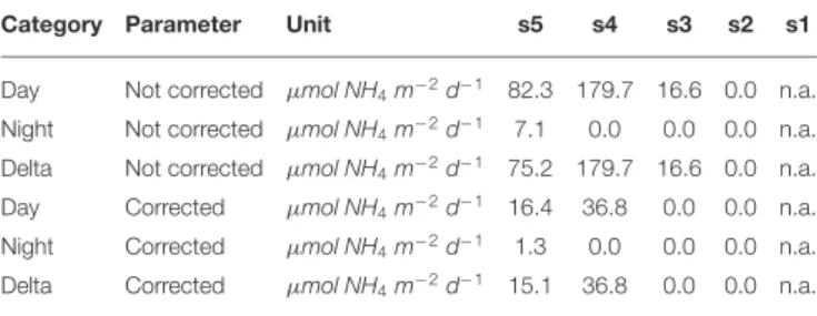
TABLE 5 | Integrated ammonium excretion rates of Euphausiacea for the 200–400 m depth level. A 12 h residence time in this layer at daytime was assumed.
Category Parameter Unit s5 s4 s3 s2 s1
Day Not corrected µmol NH4m−2d−1 82.3 179.7 16.6 0.0 n.a.
Night Not corrected µmol NH4m−2d−1 7.1 0.0 0.0 0.0 n.a.
Delta Not corrected µmol NH4m−2d−1 75.2 179.7 16.6 0.0 n.a.
Day Corrected µmol NH4m−2d−1 16.4 36.8 0.0 0.0 n.a.
Night Corrected µmol NH4m−2d−1 1.3 0.0 0.0 0.0 n.a.
Delta Corrected µmol NH4m−2d−1 15.1 36.8 0.0 0.0 n.a.
n.a., not applicalbe.
mg C m−2 d−1 for stations s3–s5 (Table 4), values that are at least 8-fold lower then those obtained omitting the necessary correction for metabolic suppression.
3.4. Ammonium Excretion of Euphausiids
Integrated ammonium excretion rates of Euphausiids for the 200–400 m depth layer are listed in Table 5. We only calculated rates for this depth interval, as the only published function to calculate oxygen-dependent ammonium excretion rates was obtained for measurements conducted at 13◦C (Kiko et al.,
2016). Mean temperatures in the 200–400 m depth layer were found to range between 10 and 16◦C. Euphausiids were observed
in this depth range at stations s3–s5. Ammonium excretion rates at daytime ranged between 0 and 36.81 µmol NH4 m−2
d−1 (n = 3), at nighttime between 0 and 1.33 µmol NH 4
m−2
d−1 (n = 3). The resulting diel vertical migration flux of
Ammonium into the 200–400 m depth layer ranged between 0 and 36.81 µmol NH4 m−2 d−1. Ammonium excretion rates
not corrected for the metabolic suppression due to hypoxia were about 4-fold higher at stations s4 and s5 than the corrected rates. At station s3, corrected rates were 0 µmol NH4 m−2d−1,
whereas the non-corrected daytime rate and DVM-related flux was 16.57 µmol NH4m−2d−1.
4. DISCUSSION
4.1. General Remarks
In the Tropical Pacific, zooplankton biomass is inversely related to depth of the thermocline and is positively related to chlorophyll, primary production and concentration of nutrients (Fernández-Álamo and Färber-Lorda, 2006). In the productive Humboldt upwelling system (HUS) off Peru, zooplankton biomass is extremely high. It is therefore very interesting to consider the role of zooplankton in the biogeochemical cycles of the HUS, both due to their local impacts on elemental cycles of e.g., carbon, nitrogen and oxygen, but also due to the possibly basin-wide implications of these impacts. Here, we focus on the impact of the OMZ on the metabolic activity of DVM organisms. Earlier estimates of zooplankton mediated fluxes to the OMZ are likewise too high, as active flux due to respiration was estimated as 0.12 times the migratory biomass (Escribano et al., 2009). The factor 0.12 stems from a global
analysis of zooplankton and biomass respiration rate data that specifically excluded upwelling areas (Hernández-León and Ikeda, 2005). It therefore seems inappropriate to apply it in upwelling systems. High active export fluxes in OMZ regions were also assumed in earlier modeling work, which also proposed that diel vertical migrants are one of the major sources of dissolved ammonium to anoxic waters as well as major consumers of oxygen at depth (Bianchi et al., 2013, 2014). For the first time, we have now incorporated metabolic suppression of migrating crustaceans (Kiko et al., 2015, 2016) into an estimate of active transport according to experimental results. Our results indicate that for OMZ regions, oxygen is a key environmental variable that does not only drive species distribution, but also scales metabolic activity, and therefore needs to be included in modeling efforts of zooplankton-mediated elemental fluxes.
4.2. Biomass Distribution Along the
Transect Sampled
According to Ayón et al. (2008) and references therein, zooplankton are numerically dominated by crustaceans off Peru. The main zooplankton groups off central Peru are copepods (which are by far the most abundant group) and euphausiids. Among those taxa that are also abundant are e.g., chaetognaths, siphonophores, polychaetes, and salps. Because some of these organisms are large, they do contribute substantially to total biomass despite their high water content. Still, we have to keep in mind that our values are likely underestimates, as also the gear in use leads to a truncated size spectrum. We did not include organisms passing through a 500 µm mesh in this analysis, and active swimming macrozooplankton/micronekton as well as rare species are not sampled quantitatively by the multinet. Despite the high upwelling and productivity at the shelf stations, total integrated biomass was lower at the two nearshore stations. This was mainly due to the dominance of small copepods, the extremely shallow oxycline and the water depth being too shallow for organisms conducting DVM, except for P. monodon, which partly resides at the seafloor during the day (Kiko et al., 2015). According toAntezana (2009), the mean daytime depth of E. mucronata is ∼250 m. At the 210 m deep station s3, integrated euphausiid biomass (and, thus, also migrant biomass) was already markedly reduced to ∼ 460 mg DW m−2,
compared to the outer stations with >1, 000 mg DW m−2(except
in the nighttime haul at s4 where only few euphausiids where caught in the surface layer). Except for that haul, the contribution of euphausiids to total well-preserved biomass at water depths >200 m ranged between 25 and 71%, which is lower than that reported byAntezana (2010) at 10◦S and 14◦S off Peru.
An increasing shelf-slope-offshore trend in epipelagic integrated biomass estimated acoustically by night was also reported for macrozooplankton off Peru (6–18◦S) by Ballón et al. (2011),
albeit with substantially higher values (around 100 g DW m−2),
since their approach included species that are capable of net avoidance (which is to some extent the case for euphausiids). In the same study, epipelagic zooplankton biomass was also determined by vertical 300 µm net hauls, and these estimates are
Kiko and Hauss Zooplankton-Mediated Fluxes in OMZs
well within the range of our values, with ∼ 1–20 g DW m−2).
Also, volume-specific euphausiid biomass in the different depth layers was ∼10 times lower compared toEscribano et al. (2009), who used a 1 m2 Tucker trawl towed at 5 kn. Thus, our calculated total biomass is well comparable to mesozooplankton estimates using other methods, but underestimates the biomass of macrozooplankton/micronekton, which is mostly due to a gear effect (avoidance of the relatively small/slow Hydrobios Multinet Maxi).
4.3. Metabolic Activity of Zooplankton Off
Peru
Depth-resolved estimates of zooplankton metabolic activity that account for the metabolic suppression due to anoxic conditions do not yet exist for the HUS. Hernández-León and Ikeda (2005)excluded the upwelling areas from their analysis of global zooplankton respiration, likely due to the lack of appropriate data. They found maximum integrated oceanic zooplankton respiration rates in the 10◦N to 20◦N latitudinal range of about
240 mg C m−2 d−1. Our corrected integrated respiration rate
estimates (only for well-preserved zooplankton, size fraction 300 − 500 µm excluded) range from 4.4 to 378.5 mg C m−2
d−1. Values at the two offshore stations s4 and s5 range between 75.4 and 112.1 mg C m−2 d−1 and are therefore within the lower
range of the estimates byHernández-León and Ikeda (2005). Low integrated rates despite extremely high biomass are due to the suppression of metabolic activity. Not corrected rates are with 105.73 to 370.68 mg C m−2
d−1 within the range reported by
Hernández-León and Ikeda (2005).
Also Ekau et al. (2018) calculated integrated zooplankton respiration rates using a constant factor of 54.6 mL O2 g−1 DM d−1 (which is ∼
2.44 µmol O2 mg−1 DM d−1) for the Benguela upwelling
system, although this system features an intense OMZ. Their values generally range between 45 and 135 µmol O2 m−2 d−1,
with maxima of 900 µmol O2m−2d−1(10.71 mg C m−2d−1).
These values likely also require a downward correction, although in this system zooplankton rather tend to avoid extremely low oxygen values, which means that metabolic suppression might not occur.
It is even more important to consider the metabolic suppression when studying DVM-mediated active export of respiratory carbon. Not considering this mechanism leads to 10-fold overestimation of DVM-mediated carbon export to below 100 m depth at stations s4 and s5. At station s3 we would assume a considerable export of 5.08 mg C m−2 d−1, where
there is none. Likewise, Escribano et al. (2009) calculated a DVM-mediated active export of 4417.4 mg C m−2
d−1 via
respiration to the 60–600 m depth layer, which should likely be reduced to zero due to the fact that the oxygen concentrations at their sampling location were extremely low between 60 and at least 500 m depth.
Another dataset of zooplankton mediated active export from an upwelling region was collected in the California Current system (Stukel et al., 2013). Here, oxygen values of about 40 µmol O2 kg−1 are found at 400 m depth (Ren et al.,
2018). These oxygen concentrations are likely high enough to allow normal respiratory activity. Stukel et al. (2013)report a DVM-mediated respiratory flux of 2.4 to 47.1 mg C m−2 d−1,
which is rather high in comparison to the corrected fluxes we observe, but would be consistent with non-corrected rates. In general, our work suggests that DVM-mediated respiratory carbon export into the OMZ is rather low in the Peruvian upwelling.
It was previously suggested that ammonium excretions by diel vertical migrant species might support anammox—a nitrogen loss process occurring in severely hypoxic to anoxic waters— to a large extent (Bianchi et al., 2014). Our first estimates of ammonium excretion by euphausiids in the Peruvian OMZ show that this is likely not the case. We do calculate integrated transport rates of 15.05 and 36.81 µmol NH4m−2d−1into the
200–400 m depth layer. This yields maximum rates of 0.008 nmol NH4L−1h−1. E. mucronata migrations are rather confined
to about 200–250 m depth. Assuming that all ammonium is released at this depth, would therefore result in ammonium release rates of 0.032 nmol NH4L−1h−1.Kalvelage et al. (2011)
list ammonium uptake rates due to anammox of 0.41 and 0.79 nmol NH4 L−1 h−1 at 180 and 250 m depth, respectively
(measured at 16◦S, 75◦W). Lam et al. (2009) provide rates of
2.5 and 3.3 nmol NH4 L−1 h−1 for the 200 and 400 m depth
level, respectively (measured at 12◦S, 78◦W). Our maximum
ammonium supply estimates therefore can not sustain these anammox rates, suggesting that anammox is fueled by other ammonium sources.
4.4. Implications for Zooplankton
Ecophysiology
This work relies on the summary of respiration rate estimates for different zooplankton functional groups described byIkeda (2014). Further efforts are needed to integrate novel data, to refine and to test these functions. E.g., Ikeda (2014) mostly used closed bottle approaches with several individuals for his measurements. However, work on single individuals using Clarke-type sensors (e.g.,Maas et al., 2012; Seibel et al., 2018) or optodes (e.g., Kiko et al., 2016) enables more detailed studies of e.g., the pcrit and avoids crowding effects. Especially
the temperature dependence of the pcrit, but also large scale
geographical differences in pcrit require further study. Likewise,
further measurements of ammonium excretion at different oxygen and temperature levels are needed.
One important aspect of DVM into severely hypoxic or even anoxic depth layers is the build-up of an oxygen debt through the accumulation of metabolic waste products during the stay at depth. The ability of E. mucronata to survive anoxia is likely a result of an efficient anoxic metabolism, as high lactate dehydrogenase levels are reported for this species (Gonzalez and Quiñones, 2002). Migrating organisms need to get rid of the metabolic waste products (e.g., lactate) upon return to well-oxygenated surface water, which might lead to an increase in metabolic activity following OMZ exposure. Chaston (1969)
reports a doubling of the respiration rate within the first hour after return from anoxia to normoxia in Cyclops varicans. How
metabolic activity changes in diel vertical migrators upon return to the oxic region therefore requires further study, as such an activity increase will result in a retention of metabolic activity in the oxygenated region.
4.5. Implications for Zooplankton Sampling
Currently, published datasets are often either taxonomically well-resolved abundance data, lacking information on size and biomass of the identified groups (e.g.,Criales-Hernández et al., 2008in the same region as the present study), or only contain bulk zooplankton biomass (or biovolume) data, which do not allow for the consideration of the impact of size distribution or taxonomic and functional composition on metabolic rates and fluxes as well as food web interactions (Ayón et al., 2011). Physiological rates generally do not scale linearly with body size (Moloney and Field, 1989) and therefore changes in the size distribution can go in hand with changes in zooplankton mediated biogeochemical fluxes despite unchanged bulk biomass. Detailed taxonomic analyses are very valuable for diversity studies, but it would be interesting to also integrate size measurements (e.g., via imaging) into the laboratory routine to enable individual-based studies on biogeochemical fluxes. The necessity for bulk measurements should be carefully assessed and best be accompanied by measurements of the size distribution, e.g., with imaging approaches.
One restriction of our analysis is the use of vertically hoisted, integrating nets for our sampling. Apart from missing the fragile part of the zooplankton community which is destroyed by nets (Hoving et al., 2018), net catches integrate over a range of environmental conditions, e.g., a temperature and oxygen gradient at the oxycline. The exact location of an organism and the environmental conditions where it was active can not be retrieved with integrating nets and our metabolic rate estimates are rather uncertain when the net integrated over a strong vertical gradient of temperature and/or oxygen. Optical in situ observations, e.g., using a VPR or a UVP5, Pelagios, ROVs, etc. will be helpful to ameliorate both problems, but do have the problem of instrument avoidance by optically orienting organisms (e.g., Benoit-Bird et al., 2010). In general, both approaches should be combined, optimally in an integrated camera-net instrument package to obtain a more complete understanding of zooplankton distribution.
We base our calculations on area-biomass functions obtained in the subtropical Atlantic, and the work by Lehette and Hernández-León (2009) is to our knowledge the only comprehensive work assessing this issue. Further work on area-biomass relationships is needed and the underlying individual raw data (images, weights and any further information, such as C-, N-, P-content) should be stored in an international database [e.g., in EcoTaxa (Picheral et al., 2019)], similar to the NCBI database of genomic sequences. Such data will enable us to better unlock the secrets that are hidden in the image data from the zooscan approach and other optical methods that are currently being collected. Also for these data, EcoTaxa seems to be the currently best developed solution for image hosting, collaborative online sorting and data sharing. Some of these ideas have already been discussed inLombard et al. (2019), an outlook
paper that details the needs for a globally consistent strategy in plankton ocean observation, but the need for a database that contains individual high-quality images and data should not be overlooked.
4.6. Implications for Other Regions, Global
Biogeochemistry, and Modeling
Our sampling is restricted to a very small area and our estimates are only valid for the HUS region where oxygen levels go down to almost anoxic levels. Metabolic suppression effects are obviously strongest in this region, leading to an almost complete shutdown of metabolic activity. Similar effects are to be expected for the northern part of the Indian Ocean, the Black sea, the Baltic sea and other severe OMZs. Regions further offshore, as well as north and south of our sampling region feature less severe OMZ conditions. This might enable stronger DVM activity, also by taxonomic groups other than euphausiids, which might also feature different pcrit values (Seibel et al., 2016). It
seems necessary to specifically map the zooplankton community composition and the metabolic capacities of DVM-organisms in transitional areas between extreme OMZs and well-oxygenated waters in order to better estimate zooplankton-mediated impacts on OMZ biogeochemistry.
Currently, the global ocean is losing oxygen and midwater OMZs are intensifying and expanding under global warming conditions (Stramma et al., 2008; Schmidtko et al., 2017) due to changes in ocean mixing and reduced oxygen solubility (Matear and Hirst, 2003; Bopp et al., 2013; Cocco et al., 2013). Large scale feedbacks between changing oxygen levels and the role of zooplankton in the elemental cycling of oxygen, carbon and nitrogen are to be expected. Oxygen levels in less extreme oceanic OMZ regions may in the near future fall below the pcrit of vertically migrating species. Oxygen loss
will likely result in a dampening of zooplankton metabolic activity in OMZ regions, first via avoidance of the OMZ by non-tolerant species and second through metabolic suppression in tolerant species. Respiration activity of zooplankton should therefore decline with declining OMZ oxygen levels. The zooplankton community composition could be a relevant factor in determining the deoxygenation rate and might influence if an OMZ stabilizes at a region-specific oxygen level. Feedbacks on nutrient cycling might include the retention of nitrogen in the surface layer, as ammonium excretion at depth is reduced.
It seems critical that metabolic suppression in DVM organisms is also considered in efforts to model the role of zooplankton organisms in biogeochemical cycles. Bianchi et al. (2013) and Bianchi et al. (2014) did not take this into account and used a model formulation that resulted in a linear relationship between passive particle export and oxygen utilization or ammonium release. Their zooplankton-mediated fluxes are likely too high in extreme OMZ regions. Aumont et al. (2018) and Archibald et al. (2019) on the other hand impose minimum oxygen thresholds of 5 µmol O2 kg−1 and
15 µmol O2kg−1, respectively below which migratory organisms
Kiko and Hauss Zooplankton-Mediated Fluxes in OMZs
model formulation would otherwise predict negative oxygen concentrations due to ongoing respiration. The parameterization with a fixed oxygen threshold might result in an appropriate estimation of metabolic rates (but for the wrong reasons), as migrating organisms are artificially displaced to shallower depth levels, where e.g., temperatures are generally higher and therefore metabolic rate estimates elevated. The inappropriate displacement of the DVM organisms might also result in other errors in the model, e.g., the gut flux and mortality occur at shallower depth. Using our approach to account for downregulated metabolic activity below the pcrit might yield a
more realistic model formulation. In general, we hope that our first oxygen utilization and ammonium release rates for the DVM community of the HUS might help to better constrain future biogeochemical models.
DATA AVAILABILITY STATEMENT
CTD data used in this publication is available at https:// doi.pangaea.de/10.1594/PANGAEA.848017. Data from scanned zooplankton images is available at https://ecotaxa.obs-vlfr.fr/ (password protected, access provided upon reasonable request).
AUTHOR CONTRIBUTIONS
RK and HH developed the sampling plan, conducted the sampling, and performed all the sample analysis. RK developed and realized the calculation of individual-based biomass and metabolic rate estimates, including the correction for metabolic suppression. RK and HH outlined and wrote the article together.
FUNDING
This work was a contribution of the SFB 754 Climate-Biogeochemistry Interactions in the Tropical Ocean (www.sfb754.de) which was supported by the German Science Foundation (DFG).
ACKNOWLEDGMENTS
We thank the crew, chief scientists, and CTD teams of RV Meteor expedition M93. We are grateful to Svenja Christiansen and Jannik Faustmann for their help in the Zooscan lab. This work would not have been possible without the generous support by PD Dr. Frank Melzner and Prof. Dr. Ulrich Sommer.
REFERENCES
Antezana, T. (2009). Species-specific patterns of diel migration into the oxygen minimum zone by euphausiids in the humboldt current ecosystem. Prog. Oceanogr. 83, 228–236. doi: 10.1016/j.pocean.2009.07.039
Antezana, T. (2010). Euphausia mucronata: a keystone herbivore and prey of the humboldt current system. Deep Sea Res. Part II Top. Stud. Oceanogr. 57, 652–662. doi: 10.1016/j.dsr2.2009.10.014
Archibald, K. M., Siegel, D. A., and Doney, S. C. (2019). Modeling the impact of zooplankton diel vertical migration on the carbon export flux of the biological pump. Glob. Biogeochem. Cycles 33, 181–199. doi: 10.1029/2018GB005983 Auel, H., and Verheye, H. M. (2007). Hypoxia tolerance in the copepod calanoides
carinatus and the effect of an intermediate oxygen minimum layer on copepod vertical distribution in the northern Benguela current upwelling system and the Angola–Benguela front. J. Exp. Mar. Biol. Ecol. 352, 234–243. doi: 10.1016/j.jembe.2007.07.020
Aumont, O., Maury, O., Lefort, S., and Bopp, L. (2018). Evaluating the potential impacts of the diurnal vertical migration by marine organisms on marine biogeochemistry. Glob. Biogeochem. Cycles 32, 1622–1643. doi: 10.1029/2018GB005886
Ayón, P., Criales-Hernandez, M. I., Schwamborn, R., and Hirche, H.-J. (2008). Zooplankton research off Peru: a review. Prog. Oceanogr. 79, 238–255. doi: 10.1016/j.pocean.2008.10.020
Ayón, P., Swartzman, G., Espinoza, P., and Bertrand, A. (2011). Long-term changes in zooplankton size distribution in the Peruvian Humboldt current system: conditions favouring sardine or anchovy. Mar. Ecol. Prog. Ser. 422, 211–222. doi: 10.3354/meps08918
Ballón, M., Bertrand, A., Lebourges-Dhaussy, A., Gutiérrez, M., Ayón, P., Grados, D., et al. (2011). Is there enough zooplankton to feed forage fish populations off Peru? An acoustic (positive) answer. Prog. Oceanogr. 91, 360– 381. doi: 10.1016/j.pocean.2011.03.001
Benoit-Bird, K. J., Moline, M. A., Schofield, O. M., Robbins, I. C., and Waluk, C. M. (2010). Zooplankton avoidance of a profiled open-path fluorometer. J. Plankton Res. 32, 1413–1419. doi: 10.1093/plankt/fbq053
Bertrand, A., Ballón, M., and Chaigneau, A. (2010). Acoustic observation of living organisms reveals the upper limit of the oxygen minimum zone. PLoS ONE 5:e10330. doi: 10.1371/journal.pone.0010330
Bianchi, D., Babbin, A. R., and Galbraith, E. D. (2014). Enhancement of anammox by the excretion of diel vertical migrators. Proc. Natl. Acad. Sci. U.S.A. 111, 15653–15658. doi: 10.1073/pnas.1410790111
Bianchi, D., Galbraith, E. D., Carozza, D. A., Mislan, K., and Stock, C. A. (2013). Intensification of open-ocean oxygen depletion by vertically migrating animals. Nat. Geosci. 6, 545–548. doi: 10.1038/ngeo1837
Bianchi, D., and Mislan, K. A. S. (2016). Global patterns of diel vertical migration times and velocities from acoustic data. Limnol. Oceanogr. 61, 353–364. doi: 10.1002/lno.10219
Bopp, L., Resplandy, L., Orr, J. C., Doney, S. C., Dunne, J. P., Gehlen, M., et al. (2013). Multiple stressors of ocean ecosystems in the 21st century: projections with cmip5 models. Biogeosciences 10, 6225–6245. doi: 10.5194/bg-10-6225-2013
Chaston, I. (1969). Anaerobiosis in cyclops varicans1. Limnol. Oceanogr. 14, 298–301.
Chavez, F. P., and Messié, M. (2009). A comparison of eastern boundary upwelling ecosystems. Prog. Oceanogr. 83, 80–96. doi: 10.1016/j.pocean.2009.07.032 Childress, J. J., and Seibel, B. A. (1998). Life at stable low oxygen levels: adaptations
of animals to oceanic oxygen minimum layers. J. Exp. Biol. 201, 1223–1232. Cocco, V., Joos, F., Steinacker, M., Frölicher, T., Bopp, L., Dunne, J., et al.
(2013). Oxygen and indicators of stress for marine life in multi-model global warming projections. Biogeosciences 10, 1849–1868. doi: 10.5194/bg-10-1849-2013
Criales-Hernández, M., Schwamborn, R., Graco, M., Ayón, P., Hirche, H.-J., and Wolff, M. (2008). Zooplankton vertical distribution and migration off central Peru in relation to the oxygen minimum layer. Helgoland Mar. Res. 62:85. doi: 10.1007/s10152-007-0094-3
Czeschel, R., Stramma, L., Schwarzkopf, F. U., Giese, B. S., Funk, A., and Karstensen, J. (2011). Middepth circulation of the eastern tropical South Pacific and its link to the oxygen minimum zone. J. Geophys. Res. Oceans 116:C01015. doi: 10.1029/2010JC006565
Deutsch, C., Ferrel, A., Seibel, B., Pörtner, H. O., and Huey, R. B. (2015). Climate change tightens a metabolic constraint on marine habitats. Science 348, 1132– 1135. doi: 10.1126/science.aaa1605
Ekau, W., Auel, H., Hagen, W., Koppelmann, R., Wasmund, N., Bohata, K., et al. (2018). Pelagic key species and mechanisms driving energy flows in the northern Benguela upwelling ecosystem and
their feedback into biogeochemical cycles. J. Mar. Syst. 188, 49–62. doi: 10.1016/j.jmarsys.2018.03.001
Escribano, R., Hidalgo, P., and Krautz, C. (2009). Zooplankton associated with the oxygen minimum zone system in the northern upwelling region of chile during march 2000. Deep Sea Res. II Top. Stud. Oceanogr. 56, 1083–1094. doi: 10.1016/j.dsr2.2008.09.009
Fernández-Álamo, M. A., and Färber-Lorda, J. (2006). Zooplankton and the oceanography of the eastern tropical Pacific: a review. Prog. Oceanogr. 69, 318–359. doi: 10.1016/j.pocean.2006.03.003
Gonzalez, R. R., and Quiñones, R. A. (2002). Ldh activity in Euphausia mucronata and Calanus chilensis: implications for vertical migration behaviour. J. Plankton Res. 24, 1349–1356. doi: 10.1093/plankt/24.12.1349
Gorsky, G., Ohman, M. D., Picheral, M., Gasparini, S., Stemmann, L., Romagnan, J.-B., et al. (2010). Digital zooplankton image analysis using the zooscan integrated system. J. Plankton Res. 32, 285–303. doi: 10.1093/plankt/fbp124 Grasshoff, K., Kremling, K., and Ehrhardt, M. (2009). Methods of Seawater
Analysis. Weinheim: John Wiley & Sons.
Hernández-León, S., and Ikeda, T. (2005). A global assessment of mesozooplankton respiration in the ocean. J. Plankton Res. 27, 153–158. doi: 10.1093/plankt/fbh166
Hoving, H.-J. T., Christiansen, S., Fabrizius, E., Hauss, H., Kiko, R., Linke, P., et al. (2018). The pelagic in situ observation system (pelagios) to reveal biodiversity, behavior and ecology of elusive oceanic fauna. Ocean Sci. 15, 1327–1340. doi: 10.5194/os-15-1327-2019
Ianson, D., George A. Jackson, G. A., Angel, M. V., Lampitt, R. S., and Burd, A. B. (2004). Effect of net avoidance on estimates of diel vertical migration. Limnol. Oceanogr. 49, 2297–2303. doi: 10.4319/lo.2004.49.6.2297
Ikeda, T. (1985). Metabolic rates of epipelagic marine zooplankton as a function of body mass and temperature. Mar. Biol. 85, 1–11.
Ikeda, T. (2014). Respiration and ammonia excretion by marine metazooplankton taxa: synthesis toward a global-bathymetric model. Mar. Biol. 161, 2753–2766. doi: 10.1007/s00227-014-2540-5
Kalvelage, T., Jensen, M. M., Contreras, S., Revsbech, N. P., Lam, P., Günter, M., et al. (2011). Oxygen sensitivity of anammox and coupled n-cycle processes in oxygen minimum zones. PLoS ONE 6:e29299. doi: 10.1371/journal.pone.0029299
Kalvelage, T., Lavik, G., Jensen, M. M., Revsbech, N. P., Löscher, C., Schunck, H., et al. (2015). Aerobic microbial respiration in oceanic oxygen minimum zones. PLoS ONE 10:e0133526. doi: 10.1371/journal.pone.0133526
Kiko, R., Hauss, H., Buchholz, F., and Melzner, F. (2016). Ammonium excretion and oxygen respiration of tropical copepods and euphausiids exposed to oxygen minimum zone conditions. Biogeosciences 13, 2241–2255. doi: 10.5194/bg-13-2241-2016
Kiko, R., Hauss, H., Dengler, M., Sommer, S., and Melzner, F. (2015). The squat lobster pleuroncodes monodon tolerates anoxic “dead zone” conditions off Peru. Mar. Biol. 162, 1913–1921. doi: 10.1007/s00227-015-2709-6
Kiørboe, T. (2013). Zooplankton body composition. Limnol. Oceanogr. 58, 1843– 1850. doi: 10.4319/lo.2013.58.5.1843
Krahmann, G. (2015). Physical oceanography during METEOR cruise M93. PANGAEA. doi: 10.1594/PANGAEA.848017
Lam, P., Lavik, G., Jensen, M. M., van de Vossenberg, J., Schmid, M., Woebken, D., et al. (2009). Revising the nitrogen cycle in the peruvian oxygen minimum zone. Proc. Natl. Acad. Sci. U.S.A. 106:4752. doi: 10.1073/pnas.0812444106 Lampert, W. (1989). The adaptive significance of diel vertical migration of
zooplankton. Funct. Ecol. 3, 21–27.
Lehette, P., and Hernández-León, S. (2009). Zooplankton biomass estimation from digitized images: a comparison between subtropical and antarctic organisms. Limnol. Oceanogr. Methods 7, 304–308. doi: 10.4319/lom.2009. 7.304
Lombard, F., Boss, E., Waite, A. M., Uitz, J., Stemmann, L., Sosik, H. M., et al. (2019). Globally consistent quantitative observations of planktonic ecosystems. Front. Mar. Sci. 6:196. doi: 10.3389/fmars.2019.00196
Longhurst, A., Bedo, A., Harrison, W., Head, E., and Sameoto, D. (1990). Vertical flux of respiratory carbon by oceanic diel migrant biota. Deep Sea Res. A Oceanogr. Res. Papers 37, 685–694.
Maas, A. E., Wishner, K. F., and Seibel, B. A. (2012). Metabolic suppression in thecosomatous pteropods as an effect of low temperature and hypoxia in the eastern tropical North Pacific. Mar. Biol. 159, 1955–1967. doi: 10.1007/s00227-012-1982-x
Matear, R. J., and Hirst, A. C. (2003). Long-term changes in dissolved oxygen concentrations in the ocean caused by protracted global warming. Glob. Biogeochem. Cycles 17:1125. doi: 10.1029/2002GB001997
Moloney, C. L., and Field, J. G. (1989). General allometric equations for rates of nutrient uptake, ingestion, and respiration in plankton organisms. Limnol. Oceanogr. 34, 1290–1299.
Picheral, M., Colin, S., and Irisson, J. (2019). Ecotaxa, A Tool for the Taxonomic Classification of Images. Available online at: https://ecotaxa.obs-vlfr.fr Ren, A. S., Chai, F., Xue, H., Anderson, D. M., and Chavez, F. P. (2018). A
sixteen-year decline in dissolved oxygen in the Central California current. Sci. Rep. 8:7290. doi: 10.1038/s41598-018-25341-8
Revsbech, N. P., Larsen, L. H., Gundersen, J., Dalsgaard, T., Ulloa, O., and Thamdrup, B. (2009). Determination of ultra-low oxygen concentrations in oxygen minimum zones by the stox sensor. Limnol. Oceanogr. Methods 7, 371–381. doi: 10.4319/lom.2009.7.371
Saltzman, J., and Wishner, K. F. (1997). Zooplankton ecology in the eastern tropical Pacific oxygen minimum zone above a seamount: 1. General trends. Deep Sea Res. I Oceanogr. Res. Papers 44, 907–930.
Schmidtko, S., Stramma, L., and Visbeck, M. (2017). Decline in global oceanic oxygen content during the past five decades. Nature 542:335. doi: 10.1038/nature21399
Seibel, B. A., Luu, B. E., Tessier, S. N., Towanda, T., and Storey, K. B. (2018). Metabolic suppression in the pelagic crab, pleuroncodes planipes, in oxygen minimum zones. Compar. Biochem. Physiol. B Biochem. Mol. Biol. 224, 88–97. doi: 10.1016/j.cbpb.2017.12.017
Seibel, B. A., Schneider, J. L., Kaartvedt, S., Wishner, K. F., and Daly, K. L. (2016). Hypoxia tolerance and metabolic suppression in oxygen minimum zone euphausiids: implications for ocean deoxygenation and biogeochemical cycles. Integr. Compar. Biol. 56, 510–523. doi: 10.1093/icb/icw091
Steinberg, D. K., and Landry, M. R. (2017). Zooplankton and the ocean carbon cycle. Annu. Rev. Mar. Sci. 9, 413–444. doi: 10.1146/annurev-marine-010814-015924
Stramma, L., Johnson, G. C., Sprintall, J., and Mohrholz, V. (2008). Expanding oxygen-minimum zones in the tropical oceans. Science 320, 655–658. doi: 10.1126/science.1153847
Stukel, M. R., Ohman, M. D., Benitez-Nelson, C. R., and Landry, M. R. (2013). Contributions of mesozooplankton to vertical carbon export in a coastal upwelling system. Mar. Ecol. Prog. Ser. 491, 47–65. doi: 10.3354/meps10453 Thomsen, S., Kanzow, T., Colas, F., Echevin, V., Krahmann, G., and Engel, A.
(2016). Do submesoscale frontal processes ventilate the oxygen minimum zone off Peru? Geophys. Res. Lett. 43, 8133–8142. doi: 10.1002/2016GL070548 Wishner, K. F., Gowing, M. M., and Gelfman, C. (1998). Mesozooplankton biomass
in the upper 1000 m in the arabian sea: overall seasonal and geographic patterns, and relationship to oxygen gradients. Deep Sea Res. II Top. Stud. Oceanogr. 45, 2405–2432.
Conflict of Interest:The authors declare that the research was conducted in the absence of any commercial or financial relationships that could be construed as a potential conflict of interest.
Copyright © 2019 Kiko and Hauss. This is an open-access article distributed under the terms of the Creative Commons Attribution License (CC BY). The use, distribution or reproduction in other forums is permitted, provided the original author(s) and the copyright owner(s) are credited and that the original publication in this journal is cited, in accordance with accepted academic practice. No use, distribution or reproduction is permitted which does not comply with these terms.