Design, Measurement, and Analysis of Oxygenated Fluid Pump System by Alexander M. Mason IV Submitted to the Department of Mechanical Engineering in Partial Fulfillment of the Requirements for the Degree of Bachelor of Science in Mechanical Engineering at the Massachusetts Institute of Technology June 2012 © 2012 Alexander M. Mason IV All rights reserved The author hereby grants to MIT permission to reproduce and to distribute publicly paper and electronic copies of this thesis document in whole or in part in any medium now known or hereafter created. Signature of Author.………. Department of Mechanical Engineering May 22, 2012 Certified by……… Alexander H. Slocum Neil and Jane Pappalardo Professor of Mechanical Engineering Thesis Supervisor Accepted by………... John H. Lienhard V Samuel C. Collins Professor of Mechanical Engineering Chairman, Undergraduate Thesis Committee
Design, Measurement, and Analysis of Oxygenated Fluid Pump by Alexander M. Mason IV Submitted to the Department of Mechanical Engineering On May 22, 2012 in Partial Fulfillment of the Requirements for the Degree of Bachelor of Science in Mechanical Engineering
ABSTRACT
The author sought out the opportunity to design and implement a system for pumping oxygenated fluid and mixing it with saline, for the purpose of providing sufficient levels of oxygen for patients undergoing forms of asphyxia. The machine is able to pump oxygenated fluid by means of a low‐density polyurethane bellows, which is powered by a stepper motor. A peristaltic pump simultaneously pumps saline fluid in another branch of the system. The two branches come together, the fluids are mixed, and bubbles are removed before the fluid is ready to be injected into a patient. Solid modeling as well as machine tools were used to create the physical structure, while LabView was used as the program regulating the controls of the device. The pump operates and can successfully mix both fluids. Flow rate can be controlled via the LabView program, and variables such as force, displacement, and flow rate can be read as outputs. The modular design of the pump allows it to be easily upgraded or altered. Because of all these features, the pump is an excellent research tool for developing a method of mixing and injecting viscous oxygenated fluid. Thesis Supervisor: Alexander H. Slocum Title: Neil and Jane Pappalardo Professor of Mechanical Engineering
Acknowledgements
To my advisor, Alexander Slocum, who has helped guide this project throughout the year and helped a great deal with the analysis portion of the project. To Nevan Hanumara, instructor in 2.750/2.752 who met with me and my team weekly to make sure we were always on track. Also, thank you to the entire PERG laboratory at MIT for their assistance with various aspects of the research.I would like to give a great amount of thanks to Bruno Piazzarolo and Kristen Peña, my colleagues, for being present in this project from the beginning. Thank you Bruno for spearheading the LabView programming, and Kristen for doing the same with measuring fluid quality. The research conducted certainly would not have been possible without your help and tireless dedication. Also, thank you to Lesley Yu, our LabView representative from National Instruments. The LabView program simply would not have come together without your help. Thank you to Dr. John Kheir, of Boston Children’s Hospital, for presenting the opportunity of creating a device that has the potential to impact the lives of so many. It has been a pleasure working under your guidance. Thanks to Blow Molded Specialties for providing excellent quality bellows samples to use in this project – pumping would not have been possible!
Contents
Abstract ... 3
Acknowledgements ... 5
Contents ... 7
Figures ... 9
Tables ... 10
Chapter 1 ... 11
1.1 Purpose ... 11
1.2 Motivation ... 11
1.3 Pump Overview ... 12
1.4 Prior Art ... 14
Chapter 2 ... 17
2.1 Design Requirements ... 17
2.1.1 Cost ... 18
2.1.2 Flow Rate ... 18
2.1.3 Mixing ... 18
2.1.4 Capacity ... 19
2.1.5 Medical-Specific Requirements ... 19
Chapter 3 ... 21
3.1 Pump Design ... 21
3.1.1 Structure ... 22
3.1.2 Bellows ... 23
3.1.3 Bellows Cap ... 25
3.1.4 Volume Calculation ... 26
3.1.5 Gliding Plate Assembly ... 31
3.1.6 Peristaltic Pump ... 33
Chapter 4 ... 37
4.1 LabView Program ... 37
4.2 Program States ... 39
Chapter 5 ... 41
5.1 Flow Rate ... 41
5.1.1 Bellows Pump ... 41
5.1.2 Peristaltic Pump ... 45
5.2 Prime Time ... 46
5.3 Flat Saline Test ... 48
5.4 Dry Run ... 49
5.5 Pump Behavior ... 50
5.5.1 Force Profile ... 51
5.5.2 Position Profile ... 52
Chapter 6 ... 53
6.1 Mixing Quality ... 53
6.2 Volume Percentage ... 53
6.3 Particle Size Distribution ... 55
6.4 Rheology ... 56
6.4.1 Rheological Profile at 90% ... 57
6.4.2 Rheological Profile at 70% ... 58
Chapter 7 ... 61
7.1 Project Summary ... 61
References ... 62
Appendix A ... 63
A.1 Motor Specifications ... 63
A.2 Bellows Volume Analysis ... 64
Appendix B ... 67
Figures
FIGURE 1.1: BELLOWS IN ITS EXPANDED STATE. ... 13
FIGURE 1.2: THE COMPLETE PUMP. ... 14
FIGURE 2.1: (A) BOTH FLUIDS UNMIXED AND (B) BOTH FLUIDS AFTER BEING PASSED THROUGH A PASSIVE HELICAL MIXER. ... 19
FIGURE 3.1: O2 PUMP SYSTEM DIAGRAM, MINUS STRUCTURAL COMPONENTS 22 FIGURE 3.2: CAD MODEL OF BASIC PUMP STRUCTURE WITH 80/20. ... 23
FIGURE 3.3: CRITICAL DIMENSIONS RELATIONSHIP FOR 1L CYLINDER ... 24
FIGURE 3.4: (A) BELLOWS CAP SOLID MODEL (B) MANUFACTURED CAP WITH O-RING ... 25
FIGURE 3.4: TWO GEOMETRIC SECTIONS COMPRISE THE ENTIRE BELLOWS VOLUME. ... 26
FIGURE 3.5: PATH OF BELLOWS TRIANGULAR PROFILE ... 27
FIGURE 3.6: MEASURED AND PREDICTED VOLUME DISPLACED OF BELLOWS 31 FIGURE 3.7: CLOSE UP OF GLIDE PLATE ASSEMBLY ... 32
FIGURE 3.8: CLOSE UP OF TWO BRANCHES OF SYSTEM AND MIXER ... 34
FIGURE 4.1: INITIALIZE/CALIBRATE TAB IN LABVIEW ... 38
FIGURE 4.2: PUMP TAB IN LABVIEW ... 38
FIGURE 4.3: LOGIC DIAGRAM OF MOTOR CONTROL (PUMPING) STATE ... 40
FIGURE 5.1: WATER DISPLACED BY BELLOWS PUMP (2/17/12) ... 43
FIGURE 5.1: AVERAGE WATER DISPLACED BY BELLOWS PUMP (2/17/12) ... 44
FIGURE 5.2: SALINE FLOW RATES THROUGH PERISTALTIC PUMP: VARIABLE INPUTS ... 47
FIGURE 5.3: FLAT SALINE BAG TEST – VOLUME DISPLACED ... 48
FIGURE 5.4: BELLOWS STIFFNESS OF TWO DIFFERENT GEOMETRIES ... 50
FIGURE 5.5: FORCE PROFILE OF BELLOWS PUMP ... 51
FIGURE 5.5: POSITION PROFILE OF BELLOWS PUMP ... 52
FIGURE 6.1: MICROSCOPIC IMAGES OF FLUID AT VARIOUS CONCENTRATIONS – (A) 90% (B) 75% (C) 50% (D) 25% ... 54
FIGURE 6.2: DISTRIBUTION OF PARTICLE DIAMETER FOR 92% CONCENTRATED FLUID ... 55
FIGURE 6.3: DR. KHEIR – RHEOLOGIC PROFILE OF FLUID ... 57
FIGURE 6.4: VISCOSITY DATA FOR 90% CONCENTRATION OF FLUID ... 58
FIGURE 6.4: VISCOSITY DATA FOR 90% CONCENTRATION OF FLUID ... 59
FIGURE A.1: HAYDON-KERK MOTOR SPECIFICATIONS – FORCE VS LINEAR VELOCITY ... 63
FIGURE A.2: HAYDON-KERK MOTOR SPECIFICATIONS – FORCE VS PULSE RATE ... 64
FIGURE C1: RECIPROCATING PUMP IDEA ... 70
Tables
TABLE 2.1: SUMMARY OF DESIGN REQUIREMENTS FOR O2 PUMP ... 17
TABLE 3.1: BELLOWS PROFILE PARAMETERS (FULLY EXPANDED STATE) ... 28
TABLE 3.2: BELLOWS VOLUME – PREDICTED AND MEASURED ... 31
TABLE 5.1: BELLOWS PUMP WITH WATER ... 42
TABLE 5.2: BELLOWS PUMP WITH WATER FLOW RATES ... 42
TABLE 5.3: PERISTALTIC PUMP WITH WATER ... 45
TABLE 5.4: PERISTALTIC PUMP WITH WATER FLOW RATES ... 45
TABLE 5.5: PERISTALTIC PUMP PRIME TIME – CONSTANT INPUT SETTING ... 47
TABLE 5.6: PERISTALTIC PUMP PRIME TIME – INCREASING INPUT SETTING 47 TABLE 6.1: MEAN AND MEDIAN PARTICLE SIZE WITH VARYING FLUID CONCENTRATION ... 56
TABLE 5.6: PERISTALTIC PUMP PRIME TIME – INCREASING INPUT SETTING 65 TABLE B.1: BUDGET AND COSTS ... 67
Chapter
1
Introduction
1.1 Purpose
The author seeks to design and build a novel pumping device, specifically for viscous, non‐ Newtonian fluids. This thesis discusses the pump as designed for a viscous, oxygenated fluid (VOF) that, when injected properly into the bloodstream, raises the levels of oxygen of the patient at a substantial rate. This injection can prevent death from a form of asphyxiation, such as cardiac arrest. Additionally, this pumping device could be used not only to characterize the VOF, but also other fluids with unknown or not well‐understood properties.1.2 Motivation
According to the Heart Rhythm Foundation, 325,000 deaths occur each year as a direct result of sudden cardiac arrest [1]. When an event like this occurs, patients who don’t die as a direct result can experience serious damage to their organs. The body’s need for oxygen is critical for survival.
Dr. John Kheir from Children’s Hospital in Boston created a compressible fluid that can re‐ oxygenate blood quickly in patients with asphyxia and cardiac arrest. The fluid itself is functional and has been shown to greatly increase the oxygen content in rabbits. In spite of these achievements, the delivery of the VOF into a human patient presents challenges. Because the fluid is highly viscous as well as compressible, a conventional pump cannot be used to deliver it into the blood stream. Existing medical pumps are expensive and can only handle incompressible fluids at relatively low flow rates. A pump that addresses these issues has the potential for being using in the medical field, particularly in emergency situations.
1.3 Pump Overview
The novelty of the pump is in its ability to pump a fluid of unknown properties and control the flow rate of the fluid as it is expelled from the system. The specific application of interest calls for pumping a viscous, non‐Newtonian fluid that is compressible. This requirement calls for a feedback control loop that can regulate the fluid’s flow rate throughout the pumping process. A load cell was chosen to measure force and to provide this feedback.
Another question that arises when considering the pump is how to pump the fluid. Several options were considered, and ultimately a positive displacement pump was chosen. The prototype uses a bellows to pump fluid. The bellows, provided by Blow Molded Specialties, is made of low‐density polyethylene (LDPE), in order to retain its original shape after being
squished. A thread lies on one end, so that it can be screwed and attached onto the rest of the assembly. Below is a picture of the bellows. Figure 1.1: Bellows in its expanded state. Other elements of the system required to pump the fluid properly are saline and the means of mixing it properly with the VOF. This was achieved by using a passive helical mixer that unites the two branches of the system (saline and VOF) using a Y‐junction. This type of mixer was chosen because it requires no additional power to operate and thoroughly mixes the fluid to be at the necessary concentration. This mixing is discussed further in section 2.1.3. A picture of the full mechanism with all components is shown in Figure 1.2.
Figure 1.2: The complete pump.
1.4 Prior Art
Due to the nature of the VOF, conventional pumps cannot regulate the flow rate of the fluid very well. Prior to designing the device, existing solutions for pumping non‐conventional fluids were explored. One pump of interest was the Belmont Rapid Infuser, made by the Belmont Corporation. This pump is capable of pumping fluids at high flow rates, heating and cooling the fluid, and also detecting the line pressure [2]. A key feature of this device that is of interest is a bubble trap that removes macro‐bubbles from the system before the fluid is injected into the patient. This feature is of great importance for the VOF because of its highly gaseous, oxygenated nature. Large bubbles need to be removed from the fluid before they areultimately injected into the patient – otherwise the large bubbles in the bloodstream could cause death. Although the Belmont Rapid Infuser has great features and is very useful in some applications, it ultimately does not fulfill the role that is needed for pumping the VOF. The device does not have a way to account for the compressible nature of the fluid, and also causes cavitation.
Another device my team and I looked at was the Enhanced ACL Repair Gun, a previous project in the 2.75 class at MIT. It consists of a small, handheld gun that mixes and heats a fluid before injecting it for use [3]. The mixing mechanism within the device inspired the use of a passive helical mixer in the pump design.
Chapter
2
System Design
2.1 Design Requirements
Upon looking at the purpose for the project, its motivation, and existing devices related to the pump, the design requirements can be addressed more thoroughly. There are several components to the design. These include cost, flow rate, mixing, capacity, and medical specific requirements. Table 2.1 summarizes the system design requirements. Table 2.1: Summary of Design Requirements for O2 Pump O2 Pump Design Requirements Cost Budget of $4000 Flow Rate VOF: 200mL/min, Saline: 50mL/min Mixing Even distribution of saline in fluid Capacity 1L of fluid injected into bloodstream Medical‐specific Sterile, macro bubbles removed2.1.1 Cost
The budget over the course of the semester was $4,000. This amount was designed to cover all expenses related to the project, including: stock hardware, machining, other forms of manufacturing, and software.
2.1.2 Flow Rate
In order to provide the patient enough oxygen to survive in the event of an emergency situation, it was chosen to pump the fluid over a five‐minute period, with a full capacity of one liter. This translates to 250ml/minute, which is the flow rate needed to sustain the body’s oxygen level for a period of time before emergency medical personnel arrive on the scene. The fluid needs to be mixed with saline in order for it to be injected at a concentration that the body can handle. The higher the concentration of VOF, the more viscous the fluid is and the more difficult it is to inject in the patient’s bloodstream. Injecting 50ml/min of saline simultaneously with 250ml/minute of VOF allows for a reasonable concentration of 83.3%.
2.1.3 Mixing
If mixed at a proper concentration, the fluid should be fit to be put in the patient’s blood stream. However, the distribution of the saline must be even throughout the VOF. This will be achieved by using a passive, helical mixer in the device. When the two branches of fluid come together, they are force to flow in and out of the helices, causing a fair amount of turbulence. Below is a figure showing an unmixed combination of saline and the VOF as well as an even mixture after being passed through the helices.(a) (b) Figure 2.1: (a) Both fluids unmixed and (b) both fluids after being passed through a passive helical mixer.
2.1.4 Capacity
As mentioned, one liter of fluid is required for the pumping device. This capacity allows the patient to receive enough oxygen in their bloodstream to sustain them during an emergency situation until more medical specialists/equipment are available.2.1.5 Medical-Specific Requirements
Because the patient is receiving a fluid that is injected directly into the body, the system of injection (the pump) must, above all else, be sterile. This requires all tubing and connection to be made out of disposable, clean material that can easily be replaced. Also, in order for the device to be safe, macro bubbles must be removed from the fluid prior to entering into the bloodstream. If this does not occur, the patient could very easily die. Some form of a bubble trap, similar to that found on the Belmont Rapid Infuser, must be placed within the system to prevent this from occurring.
Chapter
3
Pumping System
3.1 Pump Design
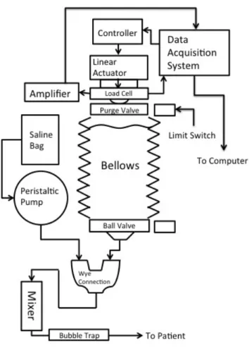
Based on the functional requirements stated above, a design was developed for the pump system. This includes the overall structure, as well as all the physical components required for functionality. The pump was built for modularity, and also to allow the flow of both the VOF and saline to be smooth such that they mix properly.Below is the overall system diagram. The diagram’s purpose is to show the major components and their spatial relation to each other. Note the relative positions of electronics, valves, switches, and reservoirs (saline and bellows). Each part of the system will be described in subsequent sections.
Figure 3.1: O2 Pump System Diagram, Minus Structural Components
3.1.1 Structure
The basic structure is comprised a series of simple, aluminum extrusions called 80/20 [5]. This material was chosen as the framework for the pump because of its modularity. Because this device was developed primary as a research tool, this feature adds to the value of the product. Many hardware changes could be made immediately simply because the connections between the pieces of the frame were relatively easy to disassemble and reassemble. Below is a screenshot from a CAD model of the pump structure.
Figure 3.2: CAD model of basic pump structure with 80/20. In addition to the 80/20 pieces, stock plates of aluminum were used on different surfaces to provide a place for other components to sit. The left portion of the structure is where the peristaltic pump is placed, as well as the saline bag. On the right, the electronics lie at the top above everything else. This decision was made in order to prevent any fluid that might leak from coming close to touching any electrical components. Below that lies the area in which the bellows sits, as well as the majority of the other mechanical components.
3.1.2 Bellows
As mentioned in Chapter 1, a bellows was chosen as the means of storing the fluid and then pumping it into the rest of the system to be mixed. LDPE was chosen because of its flexibility as a material. The bellow’s critical dimensions were determined based on its required capacity, as well as based on the control over the flow rate. For example, if for a set volume, the bellows were very large in diameter and very short in height, it would notwider base of the structure containing the bellows would be required. On the other hand, if the bellows was very tall in height but small in diameter, the stroke of the stepper motor would have to be larger, but the amount of control over how much fluid is displaced per step increases. The relationship between the critical dimensions is shown in Figure 3.3, with the region of the graph circled about where the bellows for the system lies.
Figure 3.3: Critical Dimensions Relationship for 1L Cylinder
Above, the graph simply shows the theoretical relationship between height and diameter – the bellows is approximated as a cylinder. A bellows with a somewhat larger height than diameter was chosen as a compromise between control of volume as it is expelled, and vertical space within the structure. This method is sufficient for sizing the bellows for the system, however when volume calculations come into play, a more accurate way to
0.0 1.0 2.0 3.0 4.0 5.0 6.0 7.0 8.0 9.0 10.0 3.0 3.5 4.0 4.5 5.0
Height (in.)
Diameter (in.)
Height vs Diameter for 1L Cylinder
measure volume displaced from the bellows becomes necessary. This will be explored in section 3.1.4.
3.1.3 Bellows Cap
In addition to making sure the bellows is properly sized, it is also crucial to determine how to connect the bellows to the rest of the system in a way that preserves the flow of VOF without leakage. The idea came about to create a custom cap for the bellows, which interfaces with a ball valve on one side and the threaded part of the bellows on the other. 3D printing the part allowed for more customization than fabricating the part using other methods. The critical features are: a groove for an O‐ring, internal threads to mate with the external threads of the bellows, and a hole to allow a ball valve to enter through the center of the part. Figure 3.4 shows the initial CAD design, created using Solidworks software, as well as the physical part. (a) (b) Figure 3.4: (a) Bellows Cap solid model (b) manufactured cap with O‐ringSizing the O‐ring in relation to the groove was an important part of this part’s design. It was necessary to calculate the intended compression of the O‐ring, and then using this information, to design the O‐ring to compress a given amount within the groove of the part.
3.1.4 Volume Calculation
An important aspect of the device is its ability to calculate and regulate the flow of VOF through force feedback. This is only possible if the volume of fluid expelled by the bellows is known at any given instant. With this information, calculations within LabView can happen instantaneously – a model describing the bellow’s behavior as it is compressed is needed.
The bellows can be broken up into two spatial elements: two cylinders of constant diameter, and a “rings” section where diameter oscillates between a minimum and maximum value multiple times along the bellow’s length. Figure 3.4 gives a visual representation of these two volumetric sections. Figure 3.4: Two geometric sections comprise the entire bellows volume. The volume of the two constant cylinders was calculated simply by multiplying the area of the base circle of each by their heights. Referring back to Figure 1.3, the top and bottom sections of the bellows remain unchanged as the bellows is compressed. Calculating the
volume of the rings section is trickier. The profile of each ring can be considered to be a triangle. As the bellows shrinks in size, this triangle becomes more acute, and its base shrinks linearly from its maximum to zero (Although zero cannot be the actual minimum, for the purpose of this analysis it is assumed to be in order to simplify calculations). The two legs of the triangle follow the path of a chord whose center is the outermost vertex of the profile. Figure 3.5 shows the parts of the triangular profile in detail, and Table 3.1 defines its elements. Figure 3.5: Path of Bellows Triangular Profile
Table 3.1: Bellows Profile Parameters (fully expanded state) The volume of the revolution created by the profile, as well as the inner volume between the axis of revolution and the left‐most part of the profile can be calculated using integration – more specifically the shell method. Equation 3.1 defines the shell method [6], and Equation 3.2 defines the function f (x) in the context of the triangular profile.
𝑉
!"#$%= 2𝜋 𝑟(𝑓(𝑥))𝑑𝑥
3.1𝑓 𝑥 = −
! !!𝑥 + 𝑌
3.2 B and H are values outlined in Table 3.1, and they both vary as the bellows is compressed. X is essentially r; it decreases in value as H increases. Y is the y‐intercept of the line formed by one leg of the triangle. It is equal to the slope of the line (‐B/2H) multiplied by theParameter Length (mm) Description
B 11.8
Base of triangle, which corresponds to the height of the bellows. This parameter decreases as the bellows is compressed.
S 13.8 Side of triangle. Length of this parameter is constant.
H 12.5 Height of triangle. This parameter increases as the bellows is compressed. r 45.0 Radius (not shown). This is the radius of the whole bellows, i.e. from the left‐
most point of H to the center of the bellows in Fig. 3.6.
maximum radius of the bellows. This value is the minimum radius (45mm) plus the initial length of H (12.5mm), which gives 57.5mm.
With the knowledge that the paths of each leg of the triangle are circular, the height of the triangular profile can be calculated at any level of compression (i.e. acuteness of the triangle). This means that the shell method can be used for a finite number of states of compression. A volume can be calculated for each of these states. However, this method would take a great deal of time, especially with a large number of states. Instead, the volumes of two states were calculated: one with a triangular profile representing the bellows when fully expanded, and one with a profile representing the bellows when nearly fully compressed (since complete compression is impossible if accounting for the thickness of the LDPE material). Subtracting the volumes of these two states from each other, the result is the amount of fluid displaced by one “ring”. The shell method calculations were done using a Microsoft Excel spreadsheet, and they can be found in Appendix A. Equation 3.3 summarizes integration. Note that, for simplicity, the variable Y from Equation 3.2 has been substituted by its definition in terms of the other variables.
𝑉
!"#$= 4𝜋
!"!"𝑥
!!!!𝑥 +
!!!!∗ 60 𝑑𝑥
3.3 Figure 1.3 shows that there are 10 rings that make up the bulk of the bellows’ volume, in addition to the two cylindrical sections. The volume of VOF expelled by one ring was
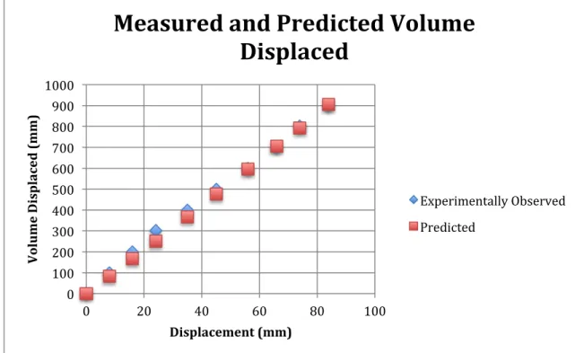
total. To test the validity of this value, the bellows was filled to its full capacity with water and then pumped throughout its entire stroke. The remaining fluid was then measured in a graduated cylinder; this value was 259 mL. Thus, the percent error of the model is 7.56%. The volume of the constant cylindrical sections was calculated to be ~921 mL. Adding this value with the measured volume of the 10 rings, the result is the total capacity of the bellows, ~1180 mL. In order to simplify the model further for the purpose of programming, an effective area was used for the calculation of the volume in the entire bellows, and then the percent error was calculated for each of these effective areas. Percent error was calculated every 2 mm the bellows was compressed, and it was found that the percent error varies through each part of the stroke. Using another Excel worksheet, all of these errors were calculated and averaged, to see which effective radius (and thus effective area) would yield, on average, the lowest percent error from the model throughout its stroke. This value was 57.9 mm, with an error of 1.038% from the model. Below in Figure 3.6 is a graphical representation of the data from the model, and how it compares to measured, real data. Table 3.2 shows the exact values.
Figure 3.6: Measured and Predicted Volume Displaced of Bellows
Table 3.2: Bellows Volume – Predicted and Measured Displacement (mm) Volume Displaced (mL) Volume Displaced Total Predicted
(mL) Percent Error (%) 0 0 0 0 8 100 82.93 1.55 16 200 166.52 3.29 24 300 250.78 5.27 35 400 367.72 3.95 45 500 475.12 3.50 56 600 594.47 0.94 66 700 704.05 0.84 74 800 792.47 1.92 84 900 903.93 1.40
3.1.5 Gliding Plate Assembly
There are a few components that constrain the bellows properly and allow it to only be unconstrained in the up and down direction. The primary mechanism that allows the
0 100 200 300 400 500 600 700 800 900 1000 0 20 40 60 80 100 Volume Displaced (mm) Displacement (mm)
Measured and Predicted Volume
Displaced
Experimentally Observed Predictedbellows and interfaces with the load cell. Beneath the bellows is a loading brace, which swings out toward the user. This piece is important because it allows the user to load the bellows without bumping into other components and without compressing the bellows before insertion into the machine. On the sides of the gliding plate are two elements: a long sliding bracket on one side, and an outrigger on the other. These pieces each have a slot that fits into a section in the 80/20 material, and allow the gliding plate to slide up and down within the structure. An outrigger was used on one side instead of two long rails in order to avoid over constraint – the outrigger is simply a small auxiliary support to avoid the bellows from twisting during compression. The figure below shows a close up of the assembly. Note the long rail on the left is about 1.6 times the radius of the gliding plate, which helped to prevent jamming, via St. Venant’s principle. Figure 3.7: Close Up of Glide Plate Assembly
Sliding
Bracket
Linear
Screw
Force
Sensor
Spacer
(Washer)
Loading
Brace
Limit
Switch
Outrigger
Amplifier
3.1.6 Peristaltic Pump
Instead of trying to invent a pump, it was decided to use pre‐existing technology for pumping saline, since it is a non‐viscous, incompressible fluid. A peristaltic pump was also chosen because it pumps within the desired flow rate range (120mL/min ‐ 2.2L/min), and the pumping action itself does not interfere with the fluid – it is a sanitary procedure. In addition, doctors are familiar with this type of pump, so it is appealing to the primary user. The pump chosen was a Thomas Scientific Mini Variable Flow Pump [7].
3.1.7 Tubing and Connections
One important part of the system is the tubing network. Each tube allows the fluid to travel easily from one component to another. Clear PVC tubing was used, as well as simple push‐ to‐connect connectors to secure the tubing. A Wye connector was used to bring together the two branches of the system (saline branch and VOF branch). A ball valve was used to interface between the bellows cap and the rest of the system. Furthermore, a bubble trap (salvaged from a Belmont Rapid Infuser) and a passive helical mixer were place in the system after the Wye connector.
Figure 3.8: Close Up of Two Branches of System and Mixer
3.2 System Fluid Model
In determining the design parameters for the system, it is necessary to look at the underlying physics in order to make informed decisions. At its essence, the pump needs to deliver fluid at a specified flow rate and mix it uniformly. Through looking at the principles that define fluid flow the power required for the device can be determined.
3.2.1 Pressure and Resistance
The transfer of power in the machine goes from electrical, in the form of a power supply, to mechanical, in the form of a lead screw drive and a bellows. Because the bellows is compressed in order to expel fluid, pressure builds up within the space. Additional
components are required, however, in order to mix the fluid, filter out bubbles, and deliver it to the patient. This requires tubing as a passage for the fluid to move through, as well as a bubble trap, fittings, and attachments. Each of these components causes friction in the path of the fluid, from the bellows to the end of the system. This friction leads to pressure build‐up, so the stepper motor must have enough power to sustain constant compression of the bellows. Each tube is idealized as a long, cylindrical pipe. Equation 3.3 is the Hagen‐Poiseuille equation, which defines the pressure drop in cylindrical pipes.
Δ𝑃 =
!!"#!!!3.3
The viscosity, μ, of the VOF was estimated to be 1000 times more viscous than water. Length L was given by the geometric constraints of the device, flow rate Q was pre‐ determined as per the functional requirements, and the radius of the tube r was given from dimensions of available medical‐grade tubing. From the equation it is clear that the radius is the most critical parameter in affecting the tube pressure, so it was chosen to be conservatively large (1/4” inner diameter) in order to minimize this. From these calculations, it was determined that there would be a pressure drop of 2.02 psi in the system, which, after multiplying by the cross sectional area, corresponds to 33 pounds of force.
With this knowledge, a Haydon‐Kerk stepper motor was chosen that could sustain 33 pounds of force without a problem. Appendix A contains motor specifications provided from the manufacturer, showing that it can provide up to 60 steady pounds of force and a maximum of 100 pounds.
Chapter
4
Programming
4.1 LabView Program
Firstly, thank you to Bruno Piazzarolo for taking the lead on this part of the project and being the primary developer of the program. During the initial development of the device, all logic and controls were done in Python, and in addition an Arduino was used to relay information from the limit switches on the device. This proved to be inefficient, as the code was not intuitive to understand and the interface was somewhat simplistic. In order to improve on this, a program in LabView was developed. This transition allowed for a high level of control with a modular and interactive interface. Instead of an Arduino, and Data Acquisition System (DAQ) was used to interface with the amplifier, load cell, and limit switches. The setup of how components connect to each other is shown above in Figure 3.1. The program interface contains two modules: one for the Initialize through Calibrate state, and one for the Pumping (Motor Control state). All the user has to do is click on one tabdistance) are all contained within the interface. The figure below shows two screenshots – one of for each tab within the front end of the program. Figure 4.1: Initialize/Calibrate Tab in LabView Figure 4.2: Pump Tab in LabView
4.2 Program States
Within the program, there are a set number of states that are executed consecutively in order to make the program run. Below is a description of what each state does.
• Initialize: checks connections and makes sure the stepper motor is ready to be operated.
• Bellows Top: the stepper motor moves downward until a non‐zero force is detected. This indicates the top of the bellows.
• Manual Jog: allows the user to manually control the position so that all the air from the bellows is purged before calibration.
• Calibration: This stage performs a test compression of the fluid and determines its compressibility curve (force vs. distance), as this may vary from batch to batch. The fluid is squished to 90% of its original volume, and then released in preparation for pumping.
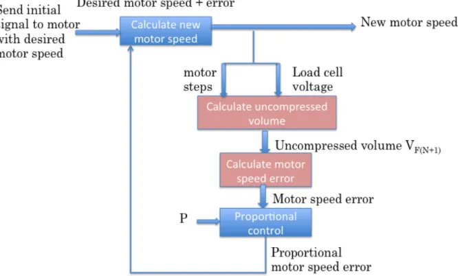
• Motor Control: This stage dispenses fluid. Error is calculated via force feedback, and the flow rate is adjusted accordingly. Proportional control is used to increase the signal from the amplifier. See Figure 4.3 for a detailed diagram. • End: cleans up the program and closes the operation of the stepper motor.
Figure 4.3: Logic Diagram of Motor Control (Pumping) State
Chapter
5
Experimentation
Once the pump was fabricated and assembled, its pumping ability was tested. A few tests were done to understand the behavior of the machine, and to see how reliable and accurate pumping can be performed.5.1 Flow Rate
The first set of these tests looks at the flow rate achieved by the pump – both the bellows pump and peristaltic. First, tests were done with water to establish a baseline of data for a Newtonian, incompressible fluid. Later, tests were done with the VOF and with another viscous fluid, corn syrup, to serve as an analogue.5.1.1 Bellows Pump
The bellows pump was filled with water before testing began. After sealing it off with the bellows cap and seal on top, it was placed underneath the stepper motor, and the stepper motor was activated. Measurements were recorded for a period of three minutes, with the volume of water expelled recorded at 20‐second intervals. The water was pumped into graduated cylinders in order to be measured accurately. By recording data in this way, itThe input flow rate was unknown for this particular test, because at the time the software program had not yet been transitioned from its old platform. However, the input voltage to the stepper motor was constant for all trials. Below is data for the initial flow rate tests with water. Table 5.1: Bellows Pump With Water Trial Time (sec) 0 20 40 60 80 100 120 140 160 180 Volume Displaced (mL) 1 0 37 70 112 145 181 219 254 ‐‐ ‐‐ 2 0 36 67 102 132 166 197 231 263 295 3 0 31 60 90 118 146 176 205 234 270 4 0 28 57 88 118 150 180 210 240 270 5 0 32 63 94 124 158 185 216 246 276 An important thing to take note of is that the final two data points for the first trial could not be recorded because the bellows ran out of fluid – not enough was put into it. Using the above data, the following flow rates were calculated: Table 5.2: Bellows Pump With Water Flow Rates Trial Average Flow Rate (mL/min) 1 108 2 98 3 90 4 90
5 92
Average 95.6
These flow rates are relatively low compared to what is required from the functional requirements, but they show that the bellows pump can pump water at relatively consistent flow rates. Graphs of the water displaced by the bellows for each trial, as well as a running calculation of the flow rate through the bellows pump over time for each trial, are shown below. Figure 5.1: Water Displaced by Bellows Pump (2/17/12) 0 50 100 150 200 250 300 350 0 20 40 60 80 100 120 140 160 180 Volume (mL) TIme (s)
Water Displaced by Bellows Pump
Trial 1 Trial 2 Trial 3 Trial 4Figure 5.1: Average Water Displaced by Bellows Pump (2/17/12) By taking a running average of the flow rate while pumping water, there is a more accurate representation of the speed and consistency of the pump over time. The data shows that, although the pump is relatively consistent in flow rate, it does vary somewhat, with a range of 87 to 108 mL/minute for trials one through four. Note: The indication of “240” in the fifth trial in Figure 5.1 indicates that the pump was run at a slightly higher flow rate (trials one through four were run at “200”). 240 is a unitless number that indicated the speed of the stepper motor when the program controlling it was written in Python. Since then the programming was transitioned to LabView, and other data, unless otherwise noted, shows the input flow rate in terms of mL/minute. 0 20 40 60 80 100 120 140 20 40 60 80 100 120 140 160 180 Flow Rate (mL/min) Time (sec)
Average Water Flow Rate Through Bellows
Pump
Trial 1 Trial 2 Trial 3 Trial 4 Trial 5 ("240")5.1.2 Peristaltic Pump
Since saline is an incompressible, Newtonian fluid that can be pumped via conventional means, a peristaltic pump was used for that branch of the system. The pump itself does not have very clearly defined input settings for flow rate – they range on a knob from zero to ten. These numbers are not useful – in order to determine how quickly saline is actually flowing into the system, another test similar to the previous one was performed. Water was pumped for three minutes and volume measurements were recorded every 20 seconds. Water was initially used instead of saline in order to establish reference data. The input setting for the pump was “8”, which, as is shown in section 5.2, corresponds to a flow rate of 71 mL/min. Below are the results. Table 5.3: Peristaltic Pump With Water Trial Time (sec) 0 20 40 60 80 100 120 140 160 180 Volume Displaced (mL) 1 0 32 63 95 128 161 192 225 256 289 2 0 28 57 84 112 142 175 206 239 270 3 0 25 50 75 100 124 149 173 197 225 4 0 29 53 80 107 133 160 186 211 237 5 0 26 52 78 105 131 157 186 217 252 Table 5.4: Peristaltic Pump With Water Flow Rates Trial Average Flow Rate (mL/min) 1 96.3
3 75 4 79 5 84 Average 84.8 The peristaltic pump tests range much more than those with the bellows. This difference in consistency can be attributed to the nature of the fluid flow. In the bellows pump setup fluid travels straight down out of the bellows and into the rest of the system. With the peristaltic pump, the tube that carries the fluid must wind around in order for it to come into contact with the rollers. This extra length of tubing as well as the turns it experiences is a cause of more friction, and thus less predictable behavior.
5.2 Prime Time
It was also important to test the prime time of each pump. Specifically, this means the time required for each pump to start up, and cause fluid to travel from its reservoir (i.e. the saline bag) out to the other end of the system. Only the prime time for the peristaltic pump was measured because of the slow rate at which it ramps up and pumps fluid relative to the bellows pump with the stepper motor. Saline was used for these tests in order to more closely represent a pumping scenario. Tables 5.5 and 5.6 show prime time at a constant input setting, as well as with increasing input settings. Measurements were taken for one minute in order to also record flow rate after the prime time was reached.Table 5.5: Peristaltic Pump Prime Time – Constant Input Setting Table 5.6: Peristaltic Pump Prime Time – Increasing Input Setting Table 5.6 shows that as the input setting increases, so does the flow rate. This correlation is best shown in graphical form, and can be seen below. 0 10 20 30 40 50 60 70 80 5 6 7 8 9 10 Flow Rate (mL/min) Input Setting
Saline Flow Rates Through Peristaltic
Pump: Variable Inputs
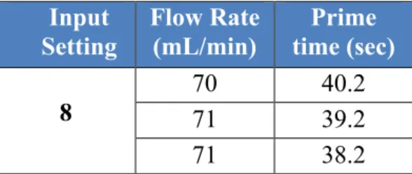
Input Setting Flow Rate (mL/min) Prime time (sec) 8 70 40.2 71 39.2 71 38.2 Input Setting Flow Rate (mL/min) Prime time (sec) 5 37 64.6 6 58 55.2 7 65 43.2 8 71 39.2 9 74 69.8 10 76 63.75.3 Flat Saline Test
In the initial assembly of the pump, the saline bag hung from the side of the structure in a vertical position, much as saline bags in hospital rooms do in an IV system. In these types of systems, the saline drips from the bag as it is delivered through a tube into the blood. The primary difference between this setting and that of the project is that instead of saline dripping, a peristaltic pump is displacing volume within the tube to draw the saline out. As the saline bag is emptied, the amount of pressure within the bag changes, causing some inconsistency in the flow rate. To address this problem, it was decided to lay the saline bag flat on a horizontal platform, so that the pressure from the fluid would vary less as the bag was emptied. This method had positive results, shown below. Figure 5.3: Flat Saline Bag Test – Volume Displaced 0 20 40 60 80 100 120 140 160 180 200 0 20 40 60 80 100 120 140 Volume (mL) Time (seconds)Flat Saline Bag Test
Trial 1 Trial 2 Trial 3 Trial 4Four trials were taken over a two‐minute period, with measurements of volume taken every ten seconds. The trend is very linear for all trials, showing that this method of positioning the saline bag is repeatable and consistent. The average flow rate for this test across all trials was 85.5 mL/min, with a standard deviation of 2.4.
5.4 Dry Run
The bellows in the system acts as a spring, compressing to expel the fluid inside it. Bellow stiffness comes into play in the software. It is important for the force the bellows exerts on the load cell to be accounted for during the calibration phase. Three bellows samples, provided by Blow Molded Specialties, were used during dry run tests. Two are “ridge” types, i.e. of the same geometry seen in Figure 1.1. One is a “corkscrew” type, which has a helical profile as part of its geometry.
All three bellows have the same expanded length, as well as the same outer and neck diameters. The only difference lies in the exterior shapes. Testing these bellows consisted of loading each one into the pump assembly, and recording the force that correlated to a distance that the bellows was displaced. The displacement ranged from zero to three inches. Below are curves showing the stiffness of each bellow. A linear relationship fit to Bellows 3 shows a relatively constant stiffness for the ridge type of geometry. This data now has use in the software for the purpose of determining the net force of the fluid in the feedback loop.
Figure 5.4: Bellows Stiffness of Two Different Geometries
5.5 Pump Behavior
“Ridge” type bellows were chosen because they are less stiff than the “corkscrew” type, and allow the stepper motor to push down on it and expel the fluid with more ease. In addition to measuring force vs. displacement, force vs. time was also measured, as well as displacement vs. time. This data indicates the bellows’ speed and how much it pushes back at a given time and position. y = 10.138x 0 5 10 15 20 25 30 35 40 45 50 55 0 0.5 1 1.5 2 2.5 3 Force (N) Displacement (inches)Bellows Stiffness
Bellows 1 (ridge) Bellows 2 (corkscrew) Bellows 3 (ridge) Linear (Bellows 3 (ridge))5.5.1 Force Profile
A few trials of the force profile were taken as the bellows was compressed with the stepper motor. The figure below shows the results. Figure 5.5: Force Profile of Bellows Pump The data shows that the force rises over time in a mostly linear fashion. Over time, and the bellows compressed near its limit, and the force increased at a much faster rate. Aside from the noise from the load cell in trial one, and change in force was relatively consistent. The maximum force recorded by the load cell was about 80 pounds, which indicates that the motor was right under its maximum load. Note the exclusion of trial two from the data. The results were very erratic and outside the norm, and the results from trials one and0 20 40 60 80 100 120 0 50 100 150 200 250 300 Force (N) Time (s)
Force Proaile
Trial 1 Trial 35.5.2 Position Profile
Data was also collected showing the position of the top of the bellows over time. This data indicates the compression of the bellows throughout the stepper motor’s stroke. Figure 5.5: Position Profile of Bellows PumpThis data was more consistent than with the force profile. This was likely because the measurement of force was more erratic – the load cell has a high degree of sensitivity. The Phidgets controller, however, was able to measure position more accurately. Again, Trial two was an outlier and was removed from the data.
0 10 20 30 40 50 60 70 0 50 100 150 200 250 300 Position (mm) Time (s)
Position Proaile
Trial 1 Trial 3Chapter
6
Fluid Quality
6.1 Mixing Quality
Firstly, thank you to Kristen Peña for leading the team in testing fluid quality. As discussed briefly in section 2.1.3, the mixing of the fluid is very important. The fluid is manufactured such that 90% of its volume is oxygenated fluid. It is then diluted with saline to be significantly less viscous before injection into the body. It is important to make sure the fluid is homogeneous so that equal amounts or oxygen are injected into the patient with each mixture. Images showing the distribution and size of bubbles for various mixtures are located in section 6.2.6.2 Volume Percentage
After taking a sample of the 90% concentrated form of the VOF, different samples were mixed at different ratios, and then viewed under a microscope to see the bubble sizes and formations. The ratios observed were various concentrations of oxygen: 90%, 75%, 50%, and 25%. Below are figures taken from Dr. Kheir’s lab at Boston Children’s Hospital via a microscope.
(a) (b) (c) (d) Figure 6.1: Microscopic Images of Fluid at Various Concentrations – (a) 90% (b) 75% (c) 50% (d) 25%
There is a clear distinction in both the size and formation of bubbles at various concentrations. The bubbles tend to be larger at higher concentrations, as well as closer together. One thing that is not easily observed is that, in Figure 6.1d, there are more than just the clusters of small bubbles. Other clusters exist, but they are out of focus. In the images of bubbles at all of the other concentrations, this same observation was made. It makes sense that the higher concentration of oxygen VOF has bubbles of larger diameters, because more oxygen is contained within a given volume.
6.3 Particle Size Distribution
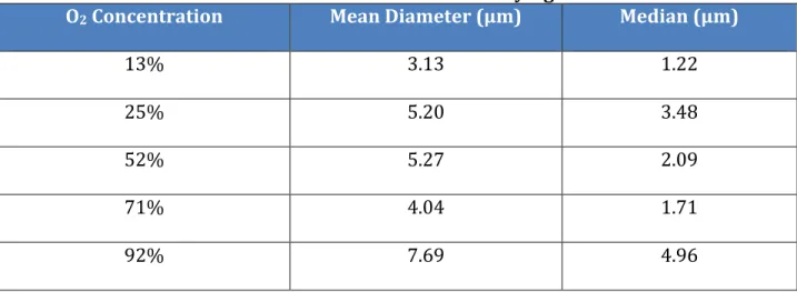
In order to understand the various particle sizes of the fluid, about a microliter of the VOF was placed into a Particle Sizer at Dr. Kheir’s lab and tested. Below is an example of one distribution of particle size from the collected data. Figure 6.2: Distribution of Particle Diameter for 92% Concentrated Fluid From the above figure, it can be seen that most particles for the 92% concentration of fluid were between 2 and 20 micrometers in diameter. The mean and other statistics regarding the data are shown. Below is a table summarizing the particle size data for all concentrations of fluid that were measured. It is important to note that the minimum particle size that the machine could possibly measure (i.e. resolution) was 0.5 micrometers.
Table 6.1: Mean and Median Particle Size With Varying Fluid Concentration O2 Concentration Mean Diameter (μm) Median (μm)
13% 3.13 1.22 25% 5.20 3.48 52% 5.27 2.09 71% 4.04 1.71 92% 7.69 4.96 These results from the particle sizer somewhat validate the claim from section 6.2, which was based on qualitative results. The mean and median values are very different in all cases – this is likely because there were multiple diameters with a spike in particle counts.
6.4 Rheology
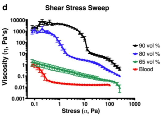
The viscosity of the VOF is very important, as it is a large factor in how well the fluid flows through the pump system. Data from Dr. Kheir shows how the fluid’s viscosity behaved after various shear stresses were applied to it [8]. This viscosity profile is shown below at different concentrations, as well as compared with blood.Figure 6.3: Dr. Kheir – Rheologic Profile of Fluid
It is clear that the VOF, especially at high concentrations, is several orders of magnitude more viscous than blood. This fact is truer at lower stresses – higher stresses cause the fluid to be less viscous. The dip in the curve for the 80% and 90% concentrated fluid represent the stresses at which each fluid yielded.
6.4.1 Rheological Profile at 90%
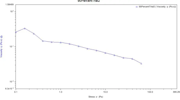
Data was collected from samples of the fluid to measure viscosity, using a rheometer in Dr. Kheir’s lab. The concentrations of interest are 90%, because that is the concentration the fluid is initially when it is manufactured, and 70%, because that is the appropriate concentration for injection into the human body. Below is rheometer data for the 90% concentration.
Figure 6.4: Viscosity Data for 90% Concentration of Fluid The fluid appears to yield the most at around 0.2 Pa. When a great amount of stress is applied, the viscosity continues to decline.
6.4.2 Rheological Profile at 70%
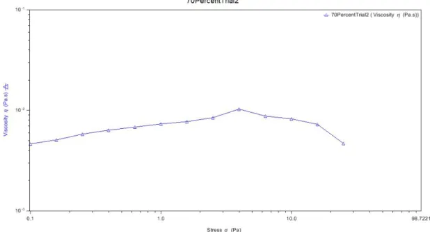
In addition, the viscosity data for the 70% concentration is shown below. The fluid does not seem to yield a great amount – in fact the viscosity increases for a large range of stress applied. After 4 Pa of pressure, the viscosity in the fluid begins to decline. Despite this, the viscosity does not change even within one order of magnitude throughout the range of stresses applied to it. This suggests that, as the fluid becomes less concentrated with oxygen, it behaves more like an incompressible fluid, and its viscosity does not change much when stress is applied to it.Figure 6.4: Viscosity Data for 90% Concentration of Fluid
Chapter
7
Conclusion
7.1 Project Summary
This thesis explored the design process, assembly, and testing of a pumping device for intravenous oxygen infusion at a specified flow rate. The flow rates measured from both the bellows pump and saline pump were consistent and desirable. Fluid flow principles, as well as volume integration assisted greatly in the analysis of the physics involved. A great deal of testing was done to validate and invalidate various approaches to the machine design.
The entire interface was created in LabView, allowing for greater ease of use, and accurate calculations of flow rate and volume displaced. When the pump was completed, it was able to pump VOF at the specified flow rate of 200mL/min, and saline at 50mL/min. The physical structure itself is stable, and uses modular materials to allow for easy reconfiguration. Various fluid properties were tested as well, to gain a great understanding of the fluid in order to pump it more efficiently. The bubble trap on the device had some
to successfully pump at mix fluid in compliance with the functional requirements. It can be used as a research tool to further understand how to better pump and mix the fluid.
References
[1] "Sudden Cardiac Arrest Key Facts." Heart Rhythm Foundation. Heart Rhythm Society. Web. 25 Apr. 2012. <http://www.heartrhythmfoundation.org/facts/scd.asp>. [2] “The Belmont Rapid Infuser”. Belmont Instrument Corporation. <http://www.belmontinstrument.com/ products/rapidInfuser>. [3] “Tool for knee surgery will help rebuild ACL”. Center for Integration of Medicine & Innovative Technology. <http://www.cimit.org/about‐stories‐kneesurgery.html>. [4] “Size 23 Stepper Motor Linear Actuator”. <http://www.haydonkerk.com>. [5] “80/20 – The Industrial Erector Set.” <http://www.8020.net/>. [6] “Oracle Thinkquest: The Shell Method” <http://library.thinkquest.org/3616/Calc/S3/TSM.html> [7] “Thomas Mini Variable Flow Pumps” < http://www.thomassci.com/Equipment/Liquid‐Pumps/_/Thomas‐Mini‐Variable‐ Flow‐Pumps/?=> [8] Kheir, John. (2011) “Device for Infusion of Intravenous Oxygen Suspension” [PowerPoint slides].Appendix
A
Analysis and Specs
A.1 Motor Specifications
Figure A.1: Haydon‐Kerk Motor Specifications – Force vs Linear Velocity The model chosen for the stepper motor is type “1” in the above figure, and can sustain a maximum of about 60 pounds of force with a step size of 0.001” [4].
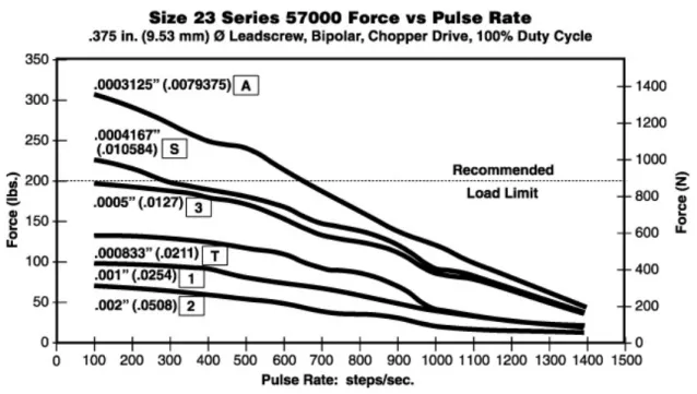
Figure A.2: Haydon‐Kerk Motor Specifications – Force vs Pulse Rate
This figure shows data for the same stepper motor, but with Pulse Rate on the x‐axis as opposed to linear velocity.
A.2 Bellows Volume Analysis
Table A.1 shows the detailed analysis of the bellows volume calculation, with a large amount of states, or iterations shown.