A Design Tool Architecture for the Rapid Evaluation of Product
Design Tradeoffs in an Internet-based System Modeling Environment
by
Jacob Wronski
Submitted to the Department of Mechanical Engineering in partial fulfillment of the requirements for the degree of
Master of Science in Mechanical Engineering OF TECHNOLOGY
at the
JUN 16 2005
MASSACHUSETTS INSTITUTE OF TECHNOLOGYMay 2005
LIBRARIES
@ Massachusetts Institute of Technology, 2005. All rights reserved.
The author hereby grants to MIT permission to reproduce and distribute publicly paper and electronic copies of this thesis document in whole or in part.
A uthor ...
Certified by...
Esther and
Accepted by ...
Chairman, Depai
Depar(e t of Mechanical Engineering May 1, 2005
David R. Wallace Harold E. Edgerton Associate Professor Thesis Supervisor
Lallit Anand rtment Committee on Graduate Students
A Design Tool Architecture for the Rapid Evaluation of Product Design Tradeoffs in an Internet-based System Modeling Environment
by
Jacob Wronski
Submitted to the Department of Mechanical Engineering on May 1, 2005, in partial fulfillment of the
requirements for the degree of Master of Science in Mechanical Engineering
Abstract
This thesis presents a computer-aided design tool for the rapid evaluation of design tradeoffs in an integrated product modeling environment. The goal of this work is to provide product development organizations with better means of exploring product design spaces so as to identify promising de-sign candidates early in the concept generation phase. Ultimately, such practices would streamline the product development process.
The proposed design tool is made up of two key components: an optimization engine, and the Dis-tributed Object-based Modeling Environment. This modeling environment is part of an ongoing research initiative at the Computer-Aided Design Lab. The optimization engine consists of a multi-objective evolutionary algorithm developed at the Ecole Polytechnique F6d6rale de Lausanne.
The first part of this thesis provides a comprehensive survey of all topics relevant to this work. Traditional product development is discussed along with some of the challenges inherent in this process. Integrated modeling tools are surveyed. Finally, a variety of optimization methods and algorithms are discussed, along with a review of commercially available optimization packages.
The second part discusses the developed design tool and the implications of this work on traditional product development. After a detailed description of the optimization algorithm, use of the design tool is illustrated with a trivial design example. Enabled by this work, a new "target-driven" design approach is introduced. In this approach, individuals select optimal tradeoffs between competing design objectives and use them, as design targets, to configure the integrated product model so as to achieve best-overall product performance. Validation of this design approach is done through the design of a hybrid PV-diesel energy system for two different applications. It is shown that the design tool effectively evaluates design tradeoffs and allows for the rapid derivation of optimal design alternatives.
Thesis Supervisor: David R. Wallace
Acknowledgments
First, I would like to thank The Center for Innovation in Product Development who, through their generosity, have made this research possible. Also, I would like to acknowledge the Ford Motor Company for providing context for this work.
I would especially like to thank my advisor, Professor David Wallace. First, for his generosity in
welcoming me to his lab and for the wonderful opportunities this experience has provided me with. Second, for his approachability and willingness to help with ideas, which made significant contri-butions to this work. Thank you.
To all my lab-mates. I would like to express my sincerest gratitude to Elaine Yang for her help in implementing some of the ideas discussed in this work. Also, to: Amy Banzaert, Qing Cao, Twiggy Chan, lason Chatzakis, Charles Dumont, Bill Fienup, Renu Fondeker, Sangmok Kim, Barry Kudrowitz, Wei Mao, Sittha Sukkasi, and Keith Thoresz. You were all a valuable part of my educa-tion at MIT.
To all my friends outside of my lab, for all the wonderful distractions you've provided me with. Especially, I would like to thank Joanna Gyory. For your kindness, encouragement ... and for mak-ing sure that I ate well while workmak-ing on this paper. I am truly blessed and honoured to have your friendship.
Finally, I would like to thank my family. To my parents, Andrzej and Maria Wronski, none of this would have ever been possible, had it not been for your love, encouragment and support! I will forever be grateful for everything you've done for me. And to my brother and sister, for your great sense of humour, which has kept me sane through some of the more difficult times.
Contents
Abstract 3 Acknowledgements 5 Contents 9 List of Figures 12 List of Tables 13 1 Introduction 15 1.1 Motivation . . . . 151.2 About this Thesis . . . . 16
1.2.1 Chapter Two: Background . . . . 16
1.2.2 Chapter Three: The Queuing Multi-Objective Optimizer . . . . 17
1.2.3 Chapter Four: Target-Driven Design . . . . 17
1.2.4 Chapter Five: Application . . . . 18
2 Background 19 2.1 Introduction . . . . 19
2.2 Product Development . . . . 19
2.2.1 Terminology . . . . 20
2.2.2 The Product Development Process . . . . 20
2.2.3 Challenges Facing Product Development Organizations . . . . 22
2.3 Design Tools For Integrated Product Modeling . . . . 24
2.3.2 DOME (Distributed Object-based Modeling Environment) . 2.4 Optimization Methods and Algorithms . . . . 2.4.1 Definition of an Optimization Problem . . . .
2.4.2 Dynamic Programming Techniques . . . . 2.4.3 Linear Optimization Techniques . . . . 2.4.4 Non-Linear or Calculus-Based Techniques . . . .
2.4.5 Enumerative Techniques . . . . 2.4.6 Heuristic Techniques . . . .
2.5 Multidisciplinary Optimization . . . .
2.5.1 Formal MDO Methods . . . .
2.5.2 Commercial Applications Providing MDO Services . . . . .
2.6 Sum m ary . . . .
3 The Queuing Multi-Objective Optimizer 3.1 Introduction ... ...
3.2 Criteria For Algorithm Selection . . . .
3.3 Design Features of the Queuing Multi-Objective Optimizer . . . . . 3.4 The Queuing Multi-Objective Optimizer . . . . 3.4.1 Assignment of Parameter Values . . . . 3.4.2 Evaluation of Objective Functions . . . .
3.4.3 Grouping . . . . 3.4.4 Ranking . . . . 3.4.5 Parent Selection . . . .
3.4.6 Thinning . . . .
3.5 Parallelism in the Queuing Multi-Objective Optimizer . . . .
3.6 Sum m ary . . . .
4 Target-Driven Design
4.1 Introduction... ...
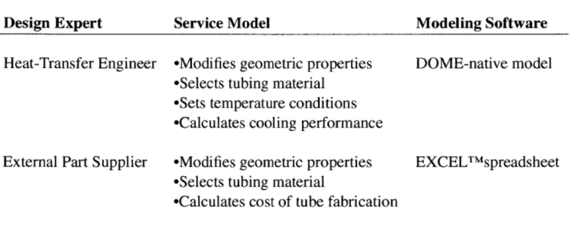
4.2 The Tube-Bundle Design Scenario . . . . 4.2.1 The "Heat Transfer Engineer" Expert . . . . 4.2.2 The "External Part Supplier" Expert . . . . 4.2.3 The Design Scenario . . . .
26 27 27 29 30 31 33 33 41 41 44 45 47 47 47 48 50 50 52 52 54 55 56 56 57 59 59 60 60 60 61
4.3 Using the DOME-enabled Optimization Tool ... ... 63
4.3.1 Building an Optimization Model . . . . 63
4.3.2 Publishing an Optimization Model on a DOME Server . . . . 69
4.3.3 Running Optimization Model Simulations . . . . 70
4.3.4 Evaluating Design Tradeoffs . . . . 72
4.4 Flow of Information Between QMOO and DOME . . . . 75
4.4.1 The DOME Evaluator Object . . . . 75
4.4.2 The DOME Monitor Object . . . . 77
4.5 Implications of Target Driven Design for Product Development . . . . 78
4.6 Summary . . . . 79
5 Application 83 5.1 Introduction . . . . 83
5.2 Design of a Hybrid PV-Diesel Energy System . . . . 84
5.2.1 Background . . . . 84
5.2.2 Design Scenario Description . . . . 85
5.2.3 Constituent Design Models . . . . 85
5.2.4 Optimization of the Design Scenario . . . . 87
5.2.5 Results . . . . 89
5.2.6 Target-Driven Design Examples . . . . 91
5.3 Summary . . . .
100
6 Conclusion 103 6.1 Summary . . . . 103
6.2 Future Work . . . . 105
6.3 Final Words . . . . 106
A Pseudo-Code for the Evaluator and Monitor Communication Objects 107 A.
1
The Evaluator Object . . . . 108A.2 The Monitor Object . . . . 111
List of Figures
2-1 The generic product development process. . . . . 20
2-2 A DOME-native volume simulation. ... 27
2-3 Subscription to a DOME-native volume simulation. . . . . 28
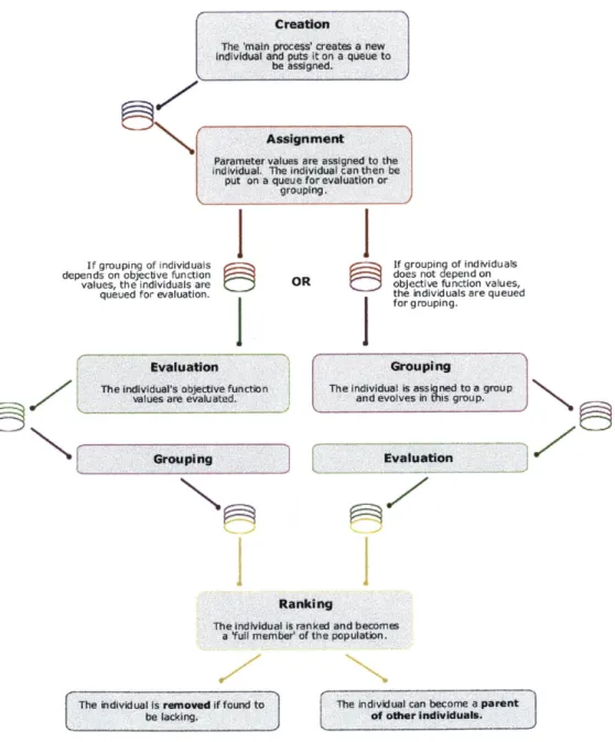
3-1 QMOO: Life of an individual. . . . . 51
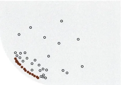
3-2 QMOO: Exploring the full range of the POF. . . . . 54
3-3 QMOO: Preservation of "tail regions". . . . . 55
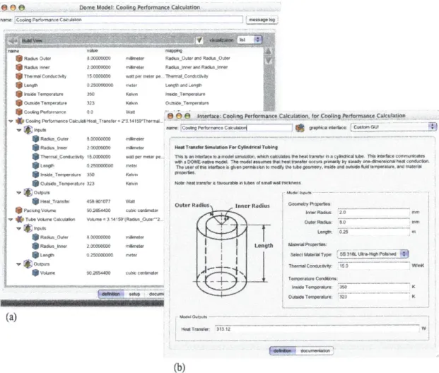
4-1 DOME-native cooling performance model. . . . . 61
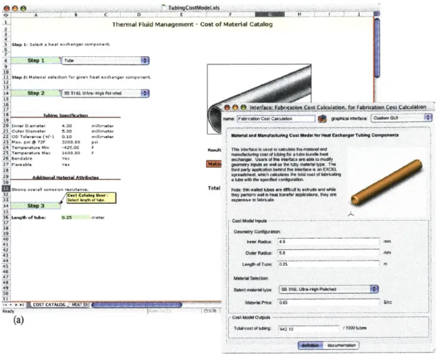
4-2 EXCELTM-native tube fabrication cost model. . . . . 62
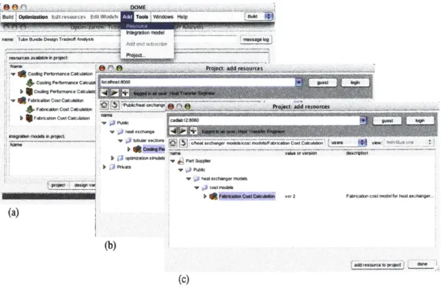
4-3 Subscribing to the cooling performance and tube fabrication cost models. . . . . . 64
4-4 Integration of the cooling performance and tube fabrication cost models. . . . . 65
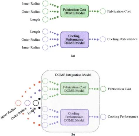
4-5 Graphical representation of the integration in the tube-bundle design scenario. . . . 66
4-6 Definition of design variables and design objectives. . . . . 67
4-7 Optimization tool configuration panel. . . . . 68
4-8 Optimization tool interfaces. . . . . 70
4-9 Optimization tool interfaces. . . . . 71
4-10 Tube-bundle design scenario Pareto fronts. . . . . 73
4-11 Selecting the target design objectives for the tube-bundle design scenario. . . . . . 74
4-12 Flow of information between QMOO and DOME. . . . . 76
5-1 Integration of the individual models in the hybrid energy system design scenario. . 87 5-2 Configuration panel of the hybrid PV-diesel energy system optimization. . . . . 89
5-3 Graphical interface to the hybrid PV-diesel energy system optimization simulation. 91 5-4 The final population of the hybrid energy system design scenario in objective space: net electricity cost vs. total CO2emission . . . . 92
5-5 The final population of the hybrid energy system design scenario in objective space:
net electricity production efficiency vs. net electricity cost . . . . 93 5-6 The final population of the hybrid energy system design scenario in objective space:
net electricity production efficiency vs. total CO2 emission . . . . 94
5-7 Individuals interacting with the hybrid energy system optimization service. . . . . 96 5-8 Using optimal tradeoffs as design targets for the design of a hybrid energy system
for a private resort application. . . . . 97 5-9 Using the net electricity cost vs. total CO2 emission optimal tradeoffs curve to
initially improve the design of a hybrid energy system for the governmental subsidy program application. . . . . 99 5-10 Using the net electricity cost vs. electricity production efficiency optimal tradeoffs
List of Tables
4.1 Description of models and expertise in the tube-bundle design scenario. . . . . 60
4.2 Contrast between the traditional engineering approach to concept development, and the optimization tool-enabled approach. Concept development stages adopted from Ulrich and Eppinger [72]. . . . . 80
5.1 Input values to the individual models in the hybrid PV-diesel energy system design scenario, taken from [70]. . . . . 86 5.2 Independent design variables and their lower/upper limits. . . . . 88 5.3 Design objectives and how each is to be optimized. . . . . 88 5.4 Initial and final design of the hybrid energy system - optimized for the private island
resort application. Units for each respective parameter are given in Figure 5-3. Improved design objectives are indicated in bold. . . . . 98 5.5 Initial and final design of the hybrid energy system - optimized for the government
subsidy program application. Units for each respective parameter are given in Fig-ure 5-3. Improved design objectives are indicated in bold. . . . . 99
Chapter 1
Introduction
1.1 Motivation
Product development firms seek to produce better performing products while reducing the time-to-market and costly design, build, test and refine cycles [77]. To achieve these objectives, various design tools and strategies are employed to accurately define the most promising concepts early in the design process. However, it has been observed that many computational tools are incapable of adapting to the dynamic and evolving nature of most product development environments and thus, the prediction of product performance early in the design process becomes a difficult task.
Organizations widely recognize the need for tools that facilitate the evaluation of integrated product performance. Thorough exploration of design alternatives early in the concept development phase reduces the likelihood that the development team will stumble on a superior design later on in the development process or that a competitor will introduce a similar product with dramatically better performance [72]. In practice, barriers such as system complexity and size, heterogeneous nature of subsystem models, and accessibility to models or expertise due to logistical and proprietary issues, greatly prohibit this approach [63]. Consequently, the evaluation of a single design candidate can take up to months to complete.
The multi-disciplinary nature of most product development teams presents a second challenge in product development, namely the management of design trade-offs in a way that maximizes the success of the product. For example, an airplane can be made lighter, but doing so will probably increase its manufacturing cost. Team members often approach such conflicts with a selfish attitude,
wishing to optimize the design objectives reflecting their own area of expertise. Clearly, this is not an acceptable approach and a better method of negotiating design tradeoffs, so as to improve the overall product performance, is needed.
To facilitate a better design approach, a design tool has been developed to rapidly evaluate and elu-cidate optimal design tradeoffs in an integrated product system model. This design tool is built into the Distributed Object-based Modeling Environment (DOME) and employs a heuristic optimization algorithm called QMOO [46]. Using the integration capabilities of DOME, the evaluation time of a single design candidate can be significantly reduced [77]. Furthermore, since the design tools employs an evolutionary algorithm to explore the design space of the product, the search for new product configurations is directed, where each new design candidate is "better" than its predeces-sors.
This thesis introduces a new design approach enabled by the design tool developed in this work. Members of a product development team can readily evaluate and obtain a graphical representation of the optimal tradeoffs of any integrated product model in the DOME framework. Furthermore, individuals can select a set of optimal design tradeoffs and use it to configure the integrated product model. The optimal design tradeoffs become the design targets for the design objectives of interest and the product system model seamlessly configures itself to satisfy these target values. "Target-driven" design and its validation in the field of product development is the main focus of this thesis.
1.2 About this Thesis
1.2.1 Chapter Two: Background
This chapter presents background topics relevant to the design tool and methodologies introduced in this work. First, the generic product development process is described and definitions of related terminology are provided. Throughout this discussion, the author presents a number of challenges, which product development organizations must overcome if they are to be successful. Next, a sur-vey of existing integrated design tools is presented with emphasis on DOME. DOME is the design framework for which the optimization tool, presented in this thesis, is developed. It was chosen for its adaptability and flexible architecture, allowing design tools to be readily implemented in its platform. Subsequently, various optimization methods and algorithms are reviewed to provide
background for the optimization engine employed by the design tool in this work. Discussed opti-mization methods include: dynamic programming, linear optiopti-mization, calculus-based, enumerative and heuristic search techniques. Finally, existing design tools with multi-disciplinary optimization capabilities are discussed and compared to the tool developed in this work.
1.2.2 Chapter Three: The Queuing Multi-Objective Optimizer
Chapter 3 presents QMOO, a multi-objective, evolutionary algorithm developed by Leyland [46].
Initially, reasons for selecting QMOO as the optimization engine are presented. Next, the design features of QMOO are discussed. QMOO is a robust, steady-state, parallel, multi-objective opti-mizer, with an asynchronous architecture that makes it quite suitable for the computation environ-ment of DOME. Following an overview of its design features, the algorithm itself is discussed in detail. Topics discussed include: assignment of parameter values, evaluation of objective functions, grouping, ranking, parent selection and thinning. Finally, design features of QMOO that allow it to run optimization problems in parallel are reviewed.
1.2.3 Chapter Four: Target-Driven Design
This chapter introduces a more effective, target-driven, approach to product design. First, a trivial design example of a tube-bundle heat exchanger is presented. Next, the optimization tool devel-oped in this work is discussed in detail. Using the design example, the author illustrates how a designer may use this tool to build an optimization model, publish it on a live Internet server, run its underlying simulation and evaluate its results. Next, the communication interface between the optimization engine, QMOO, and DOME is discussed. The DOME evaluator data object is respon-sible for sending parameter values from QMOO to an integration model in DOME, and receiving objective function values from the integration model so that they may be assigned to individuals and managed by QMOO. The DOME monitor is responsible for passing information about the op-timization solution to the designer running the simulation. Finally, implications of this work on the traditional product development process are discussed. In short, the optimization tool enables product development teams to effectively run a high number of "what-if" scenarios on a product system model. Furthermore, it rapidly evaluates and elucidates design tradeoffs, allowing the team to negotiate them in a way that is optimal with respect to the overall performance of the product.
1.2.4 Chapter Five: Application
The optimization tool has been applied to an engineering problem to validate target-driven design. This problem has been developed and studied extensively by other researchers at the CADLab. In this design scenario, the optimization tool was applied successfully and proved to be a valuable tool when assessing the performance tradeoffs between different design configurations.
The problem was originally proposed by Sukkasi [70] as part of the Alternative Energy Design
Toolkit and deals with the design of a hybrid PV-diesel energy system. Such energy systems offer
an alternative source of electricity for remote locations far from established utility grids. The PV array in the system can deliver clean electricity, but at a high capital cost. Alternatively, the diesel engine delivers inexpensive electricity, but it also taxing on the environment. The optimization con-sists of finding a number of design configurations, which produce electricity at minimum cost and impact to the environment, and then evaluating the tradeoffs between different designs.
Chapter 2
Background
2.1 Introduction
To properly introduce the design analysis tool developed in this work, and its implications on the traditional product development process, several relevant topics must first be discussed. Traditional product development process and its inherent challenges will be presented. Integrated design tools, including DOME, intended for better management and streamlining of the product development process, will be explored. The discussion will then review the more theoretical topic of optimization algorithms, to provide relevant background to the design analysis tool presented in later chapters. Finally, multidisciplinary optimization tools, similar to the one developed in this work, will be reviewed.
2.2 Product Development
This section will provide an in-depth understanding of the product development process. First, a number of definitions, used throughout this work, will be presented. Next, a generic product devel-opment process will be introduced. Finally, challenges encountered by design teams during product development will be presented.
Chapter 4 will present a design tool, developed in this work, which empowers product development teams to effectively overcome common problems (see §2.2.3) encountered in product development projects.
2.2.1 Terminology
A product in this work refers to any engineered, discrete and physical object that can be sold by an enterprise to its customers. Examples of products include kitchen appliances, sail boats, or portable computers. Product development (or design) is the sequence of steps or activities, which an enterprise employs to conceive, design, and commercialize a product [72]. Products are often developed by multidisciplinary teams with unique areas of expertise reflecting the nature of the product. They represent product development organizations and the present discussion will focus on product development in this context.
2.2.2 The Product Development Process
Product development is the process of transforming a particular costumer need to a final product or service that addresses that need [4]. It is an interdisciplinary activity requiring contributions from all functions of an organization including design, manufacturing, and product marketing. Product development is commonly viewed as an iterative design-build-test cycle driven by monetary and time constraints imposed by project management on the development team. Many generic variants of this process have been presented in literature: Ulrich and Eppinger [72], Hyman [38], Eggert [24], Cagan and Vogel [9]. Figure 2-1 illustrates one example, namely the spiral product development process, reproduced from Ulrich and Eppinger [72].
Plnig y De op et Syt vl Detail Design Ima .o. ..
Mission Concept System Spec Critical Design Production
Approval Review Review Review Approval
Figure 2-1: Process flow diagram for a generic product development process. Ulrich and Eppinger
[72] (p. 23).
Product development begins with project planning, an activity often referred to as phase zero since it precedes project approval and launch of the actual product development process [72]. This phase begins with an assessment of current technology, social trends, and economic trends for the purpose of identifying product opportunities. The output of the planning phase is a mission statement, which includes business goals, target-market for the product and anticipated challenges that will guide the development effort.
The next phase, concept development, begins with the identification of customer needs. This task is not trivial and a product developed without a good understanding of the customer will not succeed. Customers often express their preferences by describing a solution concept or an implementation approach for example, a customer might say, "I would like it to be electrically operated". A de-signer must be able to filter through such user input and obtain a need statement that is expressed in terms, independent of a particular technological solution [72]. One example of a successful product addressing a set of user needs without any preconceived hypothesis about the technology to address that need is the iMacrcomputer developed by AppleTM[9]. Designers and engineers understood that consumers were tired of the simple and dull gray desktop computers on the market. Making the iMacTMcomputer transparent and translucent and introducing candy colours was an instant success. For the first 139 days from its debut, an iMact sold at the rate of four a minute, every hour, of every day'.
Customer needs are generally expressed in the "language of the customer" [72]. While they do provide knowledge about issues of interest to the customer, they provide little guidance about how to design the actual product. Designers must effectively translate the customer needs into product target specifications a precise description of what the product has to do. Target specifications are used during the concept development phase to evaluate the relative quality of generated concepts.
The concept generation phase can be one of the most creative and rewarding activities for a prod-uct development team. It involves a mix of creative problem solving, benchmarking of competitive products, consulting with external experts and the systematic evaluation of various concepts through physical prototypes or analytical models. Typically, a development team will generate hundreds of concepts of which one will be selected for detailed design. The result of the concept development phase is a revised and detailed list of final specifications of what the product must do.
Once a design concept has been selected and final product specifications are in place, detailed de-sign takes place. At the system level, product architecture is defined and the product is fragmented into its subsystems and components. The geometry, materials, and tolerances of all components in the product are specified. Process plans for fabrication and assembly of the product are
devel-1
oped. CAD tools are used frequently to describe product geometry. Design teams often approach this phase with a "design for X" (DFX) methodology, where X may correspond to one of many criteria, such as manufacturability, environment or robustness. This often leads to competing design objectives. For example, designers often consider the cost of manufacturing a product versus its environmental impact. Such design tradeoffs are not trivial to resolve.
The testing and refinement phase involves the construction and evaluation of multiple pre-production versions of the product. Alpha and Beta prototypes of the final design are often employed at this stage to answer questions about performance and reliability.
Production ramp-up is the final phase of the product development process. At this stage, the product is entirely fabricated using the intended production system, work force is trained, and any remain-ing problems in the production process are quickly resolved. The product development process ends when the product is launched to the consumer market.
For a more comprehensive discussion of product development, the reader is referred to Ulrich and Eppinger [72].
2.2.3 Challenges Facing Product Development Organizations
Development of successful products is a difficult task. The size and scope of most product devel-opment projects creates a number of challenges for collaborative engineering in a multidisciplinary environment. This section will focus on two specific ones: (i) creating an integrated product model, and (ii) resolving design tradeoffs during product development.
The need to develop integrated models to predict the performance of a product during development is widely recognized. Computer simulations would allow design teams to run a high number of relatively inexpensive, "what-if" scenarios to determine the final product configuration. Thorough exploration of design alternatives early in the concept development phase will reduce the likeli-hood that the team will stumble upon a superior concept later in the development process or that a competitor will introduce a product with dramatically better performance [72]. In practice, compre-hensive product system modeling has been deemed infeasible [72]. Cutkosky et al. [20] identified a number of specific issues: (i) the size, complexity, and evolving nature of a product prohibits a
com-plete product model definition, (ii) members of a design team often work with different tools, data management systems and representations, and (iii) logistical and proprietary issues make global data unavailable. As a result, a single design scenario takes weeks, sometimes months, to evaluate
[77]. Product development teams often employ design-of-experiments (DOE) techniques [49, 30],
which can minimize the number of experiments required to explore the design space of the product.2 While this approach is effective, tools that allow development teams to evaluate the product system performance remain highly attractive. Cagan and Vogel [9] summarize this point succinctly:
If used correctly, [integrated product development] will significantly reduce
down-stream development problems in parts integration, manufacturing quality, and missed opportunities in style and features of the product.
Rigid product integration defines the interactions between participants and tools globally in a top-down manner. Such an approach has a significant top-downside, as it slows the organization's ability to change rapidly and be innovative, because the cost and complexity of redefining the global interac-tion model is prohibitive [77]. A variety of integrated design tools will be discussed in
§2.3.
Product development organizations often encounter design tradeoffs - inverse relationships between two specifications that are inherent in the selected product concept. For example, a design team working on a bicycle frame charged with the task of decreasing its mass is able to accomplish this task, but only with a more expensive material, such as aluminum instead of steel. Team members often approach such conflicts with a biased view, wishing to optimize design objectives that reflect their own area of expertise. Resolving such tradeoffs in a multidisciplinary development project is the most difficult part [72].
Existing integrated product modeling environments will be presented next. Chapter 4 will present a design tool developed for the DOME simulation environment, which facilitates the rapid elucidation and evaluation of optimal design tradeoffs, thus addressing the design challenges presented in this discussion.
2
DOE methods stem from robust design theory. For a more detailed discussion on this subject, the reader is referred to Phadke [59].
2.3
Design Tools For Integrated Product Modeling
Integrated product development environments offer a streamlined development process, accelerat-ing the time to market and improvaccelerat-ing product quality [63]. These drivaccelerat-ing forces are encouragaccelerat-ing research teams and commercial enterprises to develop engineering tools that can facilitate this de-velopment approach. This section will provide an overview of existing environments that allow for design collaboration and knowledge sharing in a multidisciplinary product development orga-nization. Greater detail will be afforded to the Distributed Object-based Modeling Environment (DOME), since the design tool introduced in this work was developed for this environment.
2.3.1 Collaboration-Oriented Design Tools
The SHARE project [71] is aimed to support design engineers or teams by allowing them to gather, organize, re-access and communicate design information over computer networks to establish a "shared understanding" of the design and development process. NEXT-LINK [58] incorporate agents to coordinate design decisions affected by specifications and constraints. Case and Lu [12] developed a software tool to support collaborative engineering design by treating interactions as a process of discourse. The model captures design commitments as opinions subject to review
by other designers. Agents are also used to identify conflicts between designers and to negotiate
their resolution. The Electronic Design Notebook, developed by Lewis and Singh [45], is an in-teractive electronic document, which maintains the look and feel of an engineering document to provide an integrated user interface for computer programs, design studies, planning documents, and databases. Bliznakov et al. [5] propose a design information system, which allows design-ers in a large virtual organization to indicate the status of tasks assigned to each designer or team so that other designers can follow their progress. This distributed information system is managed
by a central database. Hardwick and Spooner [34] propose an information infrastructure
archi-tecture that enhances collaboration between design and manufacturing firms. This collaboration tool uses the WWW for information sharing and the STEP standard [52] for product modeling. N-dim is a computer-based collaborative design environment for capturing, organizing and sharing data [78]. It allows participants to define information types that capture the relation between data or models. A computer-based design system DICE, developed by Sriram and Logcher [69], pro-vides a shared workspace where multiple designers work in separate engineering disciplines. DICE (Distributed and Integrated Environment for Computer-aided Engineering) implements an
object-oriented databases management system with a global control mechanism to resolve coordination and communication problems in product development projects. The design rationale provided dur-ing the product development process is also used for resolvdur-ing design conflicts [57, 56]. Xiaojuan et al. [79] are developing iShare, an Internet-based middle-ware and collaboration technology with applications in integrated modeling.
A number of design tools, which facilitate integrated product development, are available
commer-cially. FIPER®(The Federated Intelligent Product Environment), developed by Engineous Soft-wareTM, provides organizations with a design infrastructure for process integration and enterprise-wide product optimization 3. FIPER@implements a central control system, which manages work-flow, job dispatching and execution, and interactions with third-party applications. Although the models may be distributed, they are not federated. ModelCenter@is a system integration pack-age developed by Phoenix IntegrationTM.4 It implements a central "scheduler", which determines the model execution process based on a user pre-defined workflow. AML@, developed by
Tech-noSoftTM, is an object-oriented, knowledge-based engineering modeling framework. AML
imple-ments a demand-driven system solving mechanism. Given a new model state, only those models that are dependent on the change will be re-solved so that a new, consistent, system state may be obtained. This ensures the efficient use of computational resources. CO@, developed by Oculus TechnologiesTM, is an ad-hoc, peer-to-peer system integration tool5. CO integrates creates dynamic links between third party applications and propagates parameter value changes across those links.
CO does not support any type of solving mechanism.
The different systems discussed here employ a wide variety of architectures, data models and com-munications technologies, but all rely on some form of a consolidated, explicit description of the complete integrated system model. This approach may work well for small systems, but becomes a formidable task for large-scale product development projects. The following section will discuss an integrated product-modeling environment that employs an emergent system integration approach, inspired by the World Wide Web.
3 www.engineous.com 4 www.phoenix-int.com 5 www.oculustech.com
2.3.2 DOME (Distributed Object-based Modeling Environment)
The DOME integrated modeling environment was developed at the MIT Computer-Aided Design Laboratory (CADLab) to facilitate the creation of design models that can rapidly predict integrated product performance [53, 54]. The DOME framework asserts that multidisciplinary problems can be decomposed into modular sub-problems [63]. Modularity distributes knowledge and responsi-bility among members of a product development team [72]. Individuals create design models based on their area of expertise, and make them accessible over the Internet. Individuals can also define relationships between their simulation services and the services of other simulations available on the Internet. The resultant service exchange network becomes an emergent, distributed product system model capable of predicting the integrated behaviour of a design alternative [63].
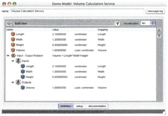
Simulation services are models that represent elements of a complete product system. The un-derlying simulation can be a third-party application, such as Excel@, Matlab@, CATIA@, or a DOME-native mathematical model. Participants that build a model (see Figure 2-2), define para-metric inputs, which drive the simulation, and parapara-metric outputs, which are the simulation results. Input-output relationships, and other implementation details about the simulation are hidden from the subscribing user, respecting proprietary issues in a product development project.
Model owners are able to define and publish parametrically operable interfaces to their simulation on the Internet. Outside users are then able to interact with the underlying simulation through this interface. Figure 2-3 illustrates the procedure that an outside user would follow to interact with the volume service simulation described above.
To build integrated simulations, participants define relationships between design models in a declar-ative fashion, which does not require knowledge about the global view of the system integration or the sequence in which the relationships should be executed. Each simulation generates and provides a causal map in its interface that relates inputs to outputs. This causal map has enough information to understand parameter changes caused by external sources, and is able to coordinate solving of the interface in an efficient manner. This distributed solving architecture can be referred to as fed-erated - models inter-operate at a global level, but maintain control at a local level. This ensures that computational efficiency is not sacrificed and the ability to detect degenerate causal structures is not lost in the emergent simulation environment. Most of all, this approach does not require the definition of a central workflow model to coordinate the solving of all relationships in the integrated
* 0Dome
Model: Volume Calculation Servicename Vokme Calculation Semce r log
Length 2. 10000000 centimeter Length Width 1 20000000 centimeter Width
Height 0400000000 centineter Height Volume 1.00800000 cubic centimeter Volume
nput -Otwt Relation Volume =LeNgtheidteHeight
Length 2.0000d00 centiviter Length
Width 1.20000000 centimeter Width
Height 0.400000od centimeter Height
'7 utpUtS
Volume 100W80000 cubic centimeter Volume
Figure 2-2: DOME-native model. This trivial service simulation calculates part volume.
model. The integrated system is able to emerge and evolve rapidly [76].
2.4
Optimization Methods and Algorithms
Numerical optimization techniques, when carefully applied, are an effective tool in engineering design. Many approaches to optimization exist, and can be grouped into five, broad categories: (i) dynamic programming, (ii) linear, (iii) non-linear or calculus-based, (iv) enumerative, and (v) heuristic6 [31]. A comparative study will reveal that each method is unique, and suitable for a
particular set of design problems. This section will review each optimization technique with fo-cus on its application to real-world engineering problems. However, before proceeding with this discussion, a formal definition of an optimization problem will be presented.
2.4.1 Definition of an Optimization Problem
A definition of a single-objective optimization problem (SOP) is provided by Vanderplaats [74]. 6
Goldberg identified the fifth optimization method as random. We will however focus on heuristic search techniques,
pft~wor DOME
fdesaent e td s tp oi Seri e vuleallotiono sevc.
(tat
DOME interface that the design participant must use to interact with the underlying simulation.
In mathematical terms, a SOP minimizes the objective function
f(x)
where x is ann-dimensional vector x = (x1,.. xn) from some design space S.
Or, in general,
minimize:
f(x)
(2.1)hx)=0x, k=1,...,m (2.4)
Equations (2.2) and (2.3) define the inequality and equality constraints, respectively. Equation (2.4) defines the lower and upper limits of the search space for each decision variable.
Therefore, given a design vector with n decision variables, one would like to find a set of values, within the specified range, such that they yield the minimum possible value off(x), while satisfying all constraints imposed on the problem.
Van Veldhuizen and Lamont [73] provide a similar definition for a multi-objective optimization
problem (MOP) - the difference being that the goal is to minimize, not one objective function, but an n-dimensional vector of objectives F(x). In a MOP, the desired result is a set of solutions, which illustrate the optimal tradeoffs between design objectives.
2.4.2 Dynamic Programming Techniques
This method is most useful in design problems configured in stages, and whose design can be char-acterized as a sequence of design decisions made in each stage. The technique can be applied to any optimum design problem for a system with n stages that requires a design decision at each stage i. The design decision at each stage transforms the condition, or state, of the system entering stage i into an outgoing state that serves as the entering state for the next stage i + 1.
The first step in formulating a dynamic programming problem is establishing a design objective (the system state) to be optimized. Although generally not applicable to multi-objective design problems, weighting could be applied to transform a multi-objective problem into a single-objective problem based on some measure of importance. Decision variables must also be selected. Finally, constraints are applied to the decision variables and the optimization problem is fully defined.
The optimization analysis involves stepping forward (or backward) through the system, and at each stage in the system calculating the design objective for all available decision variables. Design con-figuration that results in the best performance, as measured by the objective function, is selected at each stage and becomes the input for the subsequent stage. This process is repeated until the final stage of the design system is reached.
Dynamic programming is a useful engineering tool in operations research the study of optimal resource allocation. One example of its application is the planning of transmission line routes in the power industry, where one is often concerned with minimizing the cost of transmission lines.
2.4.3 Linear Optimization Techniques
This widely studied class of optimization problems involves inequality constraints, which consist of both an objective function U and a set of constraints that are linear functions of the design variables. Mathematical formulation of the linear programming problem is taken from Hyman [38]:
Minimize (or maximize) the linear objective function U(x) where x is an n-dimensional decisions variable vector x=(x1,...,xn) from some universe S, subject to m constraints. Or, in general,
n
minimize: U(x) = kizi (2.5)
i=1
n
subject to: aijxi < rj, j = ,.. (2.6)
i=1
xi > 0 (2.7)
In the above expression, aij and ki are constants presumed to have known values in any particular problem. Also, the standard form of linear programming problems requires that the design variables be non-negative, as noted by equation (2.7).
7
In linear programming problems, the optimal solutions occur at the "vertices" of a design space Therefore, instead of looking at an infinite number of possible solutions, one only has to evaluate the objective function at the corner points of the design space to discover the optimum. This has great significance on the development of an efficient linear programming algorithm.
The Simplex algorithm is a popular linear programming approach. To begin the analysis, an
ap-propriate corner point is selected and the objective function is evaluated at that point. Next, the algorithm moves along a pre-determined edge of the polygon until a vertex is reached, and the ob-jective function is evaluated at that point. The most efficient strategy is to move along an edge for which the objective function increases most rapidly. The algorithm continues to move from vertex to vertex until a maximum (or minimum) for the objective function is found.
Linear programming is limited to single-objective, linear engineering problems, for which the de-sign objective and constraints can be written in mathematical form. The optimal allocation of
ufacturing resources in a plant is one application. However, most engineering problems of interest are not linear, and even fewer can be formulated in mathematical terms. Algorithms, such as the
Sequential Linear Programming (SLP) technique developed by Kelley [40], use Taylor-series
expan-sion to approximate non-linear problems as piece-wise linear. This approach requires an advanced understanding of the design space of the engineering problem at hand, and should only be used with caution. For a more detailed description of linear programming algorithms, the reader is referred to
[15].
2.4.4 Non-Linear or Calculus-Based Techniques
Calculus-based techniques use derivatives of the objective function, to obtain the optimal system state8. They can be subdivided into two main classes: (i) direct methods, and (ii) indirect methods
[31].
Direct methods are applied to unconstrained optimization problems. They seek local optima by hopping on the objective function and moving in the direction related to the local gradient. This is simply the notion of hill climbing - to find the local best, climb the function in the steepest direction. Calculus dictates that one can expect to find the minimum or maximum of a function at a point where the gradient of the function is null. The earliest gradient algorithm known is the
steepest descent method developed by Cauchy [13] in 1847. This simple algorithm is written as follows:
Data: x0 c R"
Step 0: set i=
0
Step 1: compute the search direction
hi = -Vf (Xi) stop if Vf (xi) = 0 Step 2: compute the step size A Step 3: set
Xi+1=xi +Ahi
replace i by i+1 and go to Step 1
8Many practical parameter spaces have little respect for the notion of a derivative and the smoothness this implies
Determining the appropriate step size is perhaps the most difficult task. A small step size will result in a laborious method in reaching the function minimum, while a large step size will result in the problem minimum being missed completely. For this reason, the steepest descent method will sel-dom converge to a design space minimum. Newtons method [51] uses first and second derivatives to construct a quadratic approximation of an objective function at a specific point. This approximated function is then minimized, and the decision variables at the minimum value are used as the starting point for the next iteration. This method performs better than the steepest gradient method if the initial point is chosen close to the optimal value. The conjugate gradient method, first proposed
by Hestenes [35] in 1952, is an improvement of the steepest descent method. This method uses a
combination of the local gradient, and the gradient of the previous iteration, to determine the new direction of motion. Other, more powerful, calculus-based methods for unconstrained optimization are known as Quasi-Newton Methods. The DFP algorithm, developed by Davidon [21] and Fletcher and Powell [28], and the BFGS algorithm, developed independently by Broyden [7], Fletcher [27], Goldfarb [32] and Shanno [64] are both quasi-Newton methods. Chong and Zak [15], provide a detailed review of both algorithms.
Indirect methods are suitable for constrained optimization problems. They seek local optima by solving the usually nonlinear set of equations resulting from setting the gradient of the objective function equal to zero [31]. In constrained optimization problems, an optimum design variable vec-tor minimizes the objective function while satisfying all design constraints. Penalty and barrier
methods treat the optimization problem as unconstrained, and assign penalties to the objective
func-tion to limit constraint violafunc-tions. Carrol and Johnson [11] introduced an interesting penalty funcfunc-tion method, which has been developed extensively by Fiacco and McCormick [26] into the Sequential
Unconstrained Minimization Technique (SUMT). Sequential Quadratic Programming (SQP) [55]
was developed in the 1970s and is considered to be the most efficient gradient-based optimization technique. The method involves creating a quadratic approximation to the Lagrange-Newton for-mulation of the optimization problem and a linear approximation to the problem constraints. These equations are then solved using quadratic programming techniques until some termination criteria are reached. Method of Feasible Directions is a calculus-based optimization technique proposed Vanderplaats [74] in 1984. The optimization begins with a point in the feasible design region (no active or violated constraints), and moves in the direction of steepest descent. Conjugate direction or variable metric techniques are used on the objective function until a constraint is encountered.
At the constraint boundary, the algorithm must find a usable-feasible direction, where a usable di-rection is one that reduces the objective and a feasible didi-rection is one that either follows or moves inside a constraint boundary. This requires that a system of equations be solved numerically until some termination criteria is reached. Numerous other constrained optimization algorithms exist, in-cluding the Augment Lagrange Multiplier (ALM), the Genralized Reduced Gradient (GRG) and the
Mixed Integer Programming methods, as examples. Vanderplaats [74] describes these techniques in
detail.
Calculus-based optimization techniques have two inherent shortcomings. First, they are local in scope - the optima they seek are the best in a neighbourhood of the current point. For example, in a multimodal design space, using a gradient-based method and starting the search closer to a lower peak will cause the algorithm to completely miss the higher peak. Second, calculus-based methods depend on the existence of derivatives. Practical design spaces are fraught with discontinuities and vast multimodal, noisy search spaces. As a result, calculus-based techniques are insufficiently robust and require a high level of understanding of the design problem to which they are applied. Use of such techniques should be left to the most experienced designers.
2.4.5 Enumerative Techniques
Enumerative optimization techniques are fairly straightforward. Given a finite search space, or a discretized infinite search space, the search algorithm evaluates the objective function at every point in the space, one at a time. Although this type of "trial-and-error" search is common in engineering practice, many practical design spaces are simply too large making this method inefficient. How-ever, given infinite time, the enumerative search technique is guaranteed to locate the optimum points in the types of design spaces discussed above.
2.4.6 Heuristic Techniques
Heuristic optimization methods employ "self-educating" techniques to effectively explore the pa-rameter design space. They are self-educating because with subsequent iterations, they select design vector configurations, which result in the improved performance of the objective function. In the long run, they can be expected to do no better than enumerative schemes, but they far more efficient and practical to implement. However, in practice the best configuration of a given problem instance is seldom required. More realistically, an acceptable configuration should be produced with
rea-sonably limited computer resources. This section will present two of the most popular heuristic search techniques: (i) simulated annealing, and (ii) evolutionary algorithms. The evolutionary al-gorithms technique can be implemented with population-based alal-gorithms. Unlike gradient-based search techniques, which present a single optimum design point, population-based algorithms can present the decision maker with a set of optimal designs, which illustrate the interesting regions of the design model.
Simulated Annealing
Krikpatrick et al. [44] introduced the concept of optimization by simulated annealing in 1983. De-rived from statistical mechanics, it is a heuristic technique that mathematically mirrors the cooling of a material to a state of minimum energy. Jilla and de Weck [39] use the following analogy to describe this process:
If a liquid material (i.e. metal) cools and anneals too quickly, then the material will
solidify into a sub-optimal configuration. If the liquid material cools slowly, the crys-tals within the material will solidify optimally into a state of minimum energy (i.e. ground state). This ground state corresponds to the minimum of the cost function in an optimization problem.
Returning to optimization, simulated annealing is the process of varying a set of independent design parameters to minimize the energy state (or value) of a given objective function, subject to some annealing schedule (or termination criterion). Krikpatrick et al. [44] discuss four key elements that a formulated problem must exhibit in order to be suitable for optimization using simulated annealing. First, one must define a vector of independent parameters, which will represent the state (or config-uration) of the design inside the parameter space. Second, a random generator must be implemented to explore the neighbourhoods around existing individuals. New design points are generated by per-turbing existing individuals in one or more of the given design parameters - also called degrees of freedom. The number of design parameters allowed to undergo random perturbations must be care-fully considered. If the entire design vector is allowed to change, the simulated annealing search degenerates to a random search. The other extreme - only one parameter is allowed to change, will result in constrictive neighbourhoods, lack of diversity and limited exploration of the decision variable space. The third element that must be defined is a quantitative objective function. If the
problem of interest requires the optimization of multiple design objectives, weighting factors can be used to aggregate all of the objectives into a single objective function. The fourth element to be defined is an annealing schedule, or termination criterion. A common cooling schedule is to reduce the system temperature by a constant fraction with every generation. For example, if the system begins with a temperature of 1000, and continues at a reduction rate of 95% with each perturbation, the algorithm will run for approximately 100 generations. The system temperature also plays an im-portant role in the preservation of diversity during the optimization process. This will be discussed
shortly.
The simulated annealing algorithm is presented below:
Step 1: choose a random individual (Fi), select the initial system temperature and outline the cooling (i.e. annealing) schedule
Step 2: evaluate the system energy (i.e. objective function) of the optimization model
E(Fi)
Step 3: perturb the current individual in one or more degrees of freedom to obtain a neigh-bouring individual (Fi+1)
Step 4: evaluate the system energy of the new individual E(Pi+1)
Step 5: if E(Fi+1) < E('i), Fi+1 is the new current solution
Step 6: if E(Fi+1) > E(Fi), then accept Fri- as the new current solution with a
proba-bility e(-/T) where A = E(Fi+1) - E(Fi)
Step 7: reduce the system temperature according to the cooling schedule Step 8: terminate the algorithm when the termination criterion has been reached
The reason for accepting an inferior solution (step 6) is to prevent the algorithm from getting trapped in a local optimum. The probability of accepting an inferior solution is dependent on two parame-ters: (i) the system energy difference (A) between two neighbours, and (ii) the system temperature. Therefore, the probability of moving to a worse solution with the hope of escaping a local minimum decreases over time as the system cools. Finally, there are many items one may tailor within the al-gorithm to affect its performance, including initial system temperature, cooling schedule, and DOF within a neighbourhood.
Evolutionary algorithms (EAs) are optimization techniques inspired by organic evolution observed amongst living organisms. In evolution, genetic variability from generation to generation signif-icantly affects the probability that a given individual will survive and produce offspring. Natural selection, the mechanism of evolution, exerts survival pressure on the population and ensures that only individuals with favourable genotypes are able to reproduce successfully [60]. This process is commonly referred to as survival of the fittest. Likewise, in an EA, a population of individuals
is evolved toward the solution of an optimization problem by undergoing a number of operations,
which produce new individuals and remove existing ones [46].
An individual is a possible solution to an optimization problem. It contains a design vector x, which
represents where the individual lies in the decision variable space, and also information about its degree of optimality, usually assessed via the design objective function.
The population evolves towards better solutions by creating progeny superior in fitness to their par-ents, and removing individuals from the population found to be lacking.
New individuals are added to the population by crossover operations. Crossover involves selecting two (or more) individuals from a population and creating a child (or children) that in some way resembles its parents, much like sexual reproduction. A good implementation of an EA will use a selection scheme with bias towards better parts of the population, much like a breeder of roses will choose individuals best fitting his or her goals, to be parents for the next generation. Mutation is an important operator, which takes an individual and modifies some of its parameters, much like the natural mutation of the genetic code of an organism. In an EA, the role of mutation is to ensure preservation of diversity - the spread of the population in the search space. Mutation operators,
however, must be used cautiously. Too little mutation will lead to loss of diversity in the popula-tion resulting in the algorithm converging quickly to a narrow region of the design space, and thus getting trapped in some local optima. Too much mutation will decrease the population convergence rate, thus causing the population to explore a wide region of the design space at the expense of computational time.
Removal of individuals from the population is dependent on the structure of the EA. In generational EAs, the population is processed a generation at a time, where a number of children equal to the size
of the population is generated, and used to entirely replace the existing population. In elitist EAs, a few of the fittest individuals in the population are retained from generation to generation, acting as a marker of the best performance of the algorithm thus far. These individuals also contribute to the overall convergence of the algorithm by having more children. In steady-state EAs, individuals are added and removed from the population as necessary and very often the criteria for removal of points results in some measure of elitism.
The basic overview of EAs thus complete, the discussion will now focus on each step of the algo-rithm in greater detail. In its most general form, an EA will follow the following steps:
Step 1: define a decision variable encoding - decoding scheme Step 2: define a "fitness" function F
Step 3: initialize a population of individuals in some search space S
Step 4: generate a number of new individuals and add them to the population
Step 5: remove a number of individuals from the population, which are inferior in terms of the fitness function F
Step 6: continue until some termination criterion is reached
Encoding is used extensively in one family of EAs, namely genetic algorithms. It involves 'coding' all of the individual's decision variables into a different alphabetical representation, usually binary. The crossover and mutation operators then work directly on this new representation. Thus a mu-tation operator would choose whether or not to change a particular bit, and a crossover operator would choose individual bits from each parent. Decoding is the reverse process of encoding, where decision variables are translated back to their natural form. Binary encoding of decision variables presents a number of issues. First, the number of bits used for the representation of a real variable must be carefully chosen so as to ensure sufficient resolution of the problem's optima. Secondly, representation of integers is difficult in problems where the feasible range is not a power of 2, and requires that the integers be over specified (i.e. using more bits than is necessary). Another draw-back of encoding variables to bits is apparent in the mutation operator. Since mutation works at the bit level, a good parent with a value of
![Figure 2-1: Process flow diagram for a generic product development process. Ulrich and Eppinger [72] (p](https://thumb-eu.123doks.com/thumbv2/123doknet/14722427.570734/20.918.175.707.722.784/figure-process-diagram-generic-product-development-process-eppinger.webp)
![Figure 3-3: Preservation of "tail regions". Individuals in the boxes at the ends of the NDSS are preserved, and ranked preferring "left and up" (left box) and "right and down" (right box) [46].](https://thumb-eu.123doks.com/thumbv2/123doknet/14722427.570734/55.918.238.661.360.663/figure-preservation-regions-individuals-boxes-preserved-ranked-preferring.webp)