Detection and Characterization of Oscillating
Red Giants: First Results from the TESS Satellite
The MIT Faculty has made this article openly available.
Please share
how this access benefits you. Your story matters.
Citation
Aguirre, Víctor Silva, et al. "Detection and Characterization of
Oscillating Red Giants: First Results from the TESS Satellite." The
Astrophysical Journal Letters, 889, 2 (February 2020).© 2020 The
American Astronomical Society.
As Published
http://dx.doi.org/10.3847/2041-8213/ab6443
Publisher
American Astronomical Society
Version
Final published version
Citable link
https://hdl.handle.net/1721.1/125633
Terms of Use
Article is made available in accordance with the publisher's
policy and may be subject to US copyright law. Please refer to the
publisher's site for terms of use.
Detection and Characterization of Oscillating Red Giants: First Results from the
TESS
Satellite
Víctor Silva Aguirre1 , Dennis Stello1,2,3 , Amalie Stokholm1 , Jakob R. Mosumgaard1 , Warrick H. Ball1,4 , Sarbani Basu5 , Diego Bossini6 , Lisa Bugnet7,8 , Derek Buzasi9 , Tiago L. Campante6,10 , Lindsey Carboneau9 ,
William J. Chaplin1,4 , Enrico Corsaro11 , Guy R. Davies1,4 , Yvonne Elsworth1,4, Rafael A. García7,8 , Patrick Gaulme12,13 , Oliver J. Hall1,4 , Rasmus Handberg1 , Marc Hon2 , Thomas Kallinger14 , Liu Kang15 ,
Mikkel N. Lund1 , Savita Mathur16,17 , Alexey Mints18 , Benoit Mosser19 , Zeynep Çelik Orhan20 ,
Thaíse S. Rodrigues21 , Mathieu Vrard6,22, Mutlu Yıldız20 , Joel C. Zinn2,22,23 , Sibel Örtel20 , Paul G. Beck16,17,24 , Keaton J. Bell25,62 , Zhao Guo26 , Chen Jiang27 , James S. Kuszlewicz12 , Charles A. Kuehn28, Tanda Li1,3,4, Mia S. Lundkvist1, Marc Pinsonneault22 , Jamie Tayar29,63 , Margarida S. Cunha4,6 , Saskia Hekker1,12 , Daniel Huber29,
Andrea Miglio1,4 , Mario J. P. F. G. Monteiro6,10 , Ditte Slumstrup1,30 , Mark L. Winther1, George Angelou31 , Othman Benomar32,33 , Attila Bódi34,35, Bruno L. De Moura36, Sébastien Deheuvels37, Aliz Derekas34,38,39 , Maria Pia Di Mauro40 , Marc-Antoine Dupret41, Antonio Jiménez16,17, Yveline Lebreton19,42 , Jaymie Matthews43 , Nicolas Nardetto44 , Jose D. do Nascimento, Jr.45,46 , Filipe Pereira6,10 , Luisa F. Rodríguez Díaz1 , Aldo M. Serenelli47,48,
Emanuele Spitoni1 , Edita Stonkutė49, Juan Carlos Suárez50,51, Robert Szabó34,35, Vincent Van Eylen52 , Rita Ventura11 , Kuldeep Verma1 , Achim Weiss31 , Tao Wu53,54,55 , Thomas Barclay56,57 , Jørgen Christensen-Dalsgaard1 ,
Jon M. Jenkins58 , Hans Kjeldsen1, George R. Ricker59, Sara Seager59,60,61 , and Roland Vanderspek59 1
Stellar Astrophysics Centre(SAC), Department of Physics and Astronomy, Aarhus University, Ny Munkegade 120, DK-8000 Aarhus C, Denmark
2
School of Physics, The University of New South Wales, Sydney, NSW 2052, Australia 3
Sydney Institute for Astronomy(SIfA), School of Physics, University of Sydney, Sydney, NSW 2006, Australia 4
School of Physics and Astronomy, University of Birmingham, Birmingham B15 2TT, UK 5
Department of Astronomy, Yale University, New Haven, CT 06520, USA
6Instituto de Astrofísica e Ciências do Espaço, Universidade do Porto, Rua das Estrelas, 4150-762 Porto, Portugal 7
IRFU, CEA, Université Paris-Saclay, F-91191 Gif-sur-Yvette, France 8
AIM, CEA, CNRS, Université Paris-Saclay, Université Paris Diderot, Sorbonne Paris Cité, F-91191 Gif-sur-Yvette, France 9
Dept. of Chemistry and Physics, Florida Gulf Coast University, 10501 FGCU Boulevard South, Fort Myers, FL 33965, USA 10
Departamento de Física e Astronomia, Faculdade de Ciências da Universidade do Porto, Rua do Campo Alegre, s/n, 4169-007 Porto, Portugal 11
INAF—Osservatorio Astrofisico di Catania, Via S. Sofia, 78, I-95123 Catania, Italy 12
Max Planck Institute for Solar System Research, Justus-von-Liebig Weg 3, D-37077 Göttingen, Germany 13
Department of Astronomy, New Mexico State University, P.O. Box 30001, MSC 4500, Las Cruces, NM 88003-8001, USA 14
Institut für Astrophysik, Universität Wien, Türkenschanzstrasse 17, A-1180 Vienna, Austria 15Department of Astronomy, Beijing Normal University, 100875 Beijing, People’s Republic of China
16
Instituto de Astrofísica de Canarias, E-38200 La Laguna, Tenerife, Spain 17
Departamento de Astrofísica, Universidad de La Laguna, E-38206 La Laguna, Tenerife, Spain 18
Leibniz-Institut für Astrophysik Potsdam(AIP), An der Sternwarte 16, D-14482 Potsdam, Germany 19
LESIA, Observatoire de Paris, Université PSL, CNRS, Sorbonne Université, Université de Paris, F-92195 Meudon, France 20
Department of Astronomy and Space Sciences, Science Faculty, Ege University, 35100, Bornova,İzmir, Turkey 21
Osservatorio Astronomico di Padova—INAF, Vicolo dell’Osservatorio 5, I-35122 Padova, Italy 22
Department of Astronomy, The Ohio State University, 140 West 18th Avenue, Columbus, OH 43210, USA 23
Kavli Institute for Theoretical Physics, University of California, Santa Barbara, CA 93106, USA
24Institute of Physics, Karl-Franzens University of Graz, NAWI Graz, Universitätsplatz 5/II, A-8010 Graz, Austria 25
DIRAC Institute, Department of Astronomy, University of Washington, Seattle, WA 98195-1580, USA
26Center for Exoplanets and Habitable Worlds, Department of Astronomy and Astrophysics, 525 Davey Laboratory, The Pennsylvania State University, University Park, PA16802, USA
27
School of Physics and Astronomy, Sun Yat-Sen University, No. 135, Xingang Xi Road, Guangzhou, 510275, Peopleʼs Republic of China 28
Department of Physics and Astronomy, University of Northern Colorado, Greeley, CO 80639, USA 29
Institute for Astronomy, University of Hawaii, 2680 Woodlawn Drive, Honolulu, HI 96822, USA 30
European Southern Observatory, Alonso de Córdova 3107, Vitacura, Santiago, Chile 31
Max-Planck-Institut für Astrophysics, Karl Schwarzschild Strasse 1, D-85748, Garching, Germany 32
Solar Science Observatory, NAOJ, Mitaka, Japan 33
Center for Space Science, New York University Abu Dhabi, Abu Dhabi, UAE
34Konkoly Observatory, Research Centre for Astronomy and Earth Sciences, H-1121 Budapest, Konkoly Thege M. út 15-17, Hungary 35
MTA CSFK Lendület Near-Field Cosmology Research Group, Hungary 36
Instituto Federal do R.G. do Norte - IFRN, Brazil 37
IRAP, Université de Toulouse, CNRS, CNES, UPS, Toulouse, France 38
ELTE Eötvös Loránd University, Gothard Astrophysical Observatory, Szombathely, Hungary 39
MTA-ELTE Exoplanet Research Group, 9700 Szombathely, Szent Imre h.u. 112, Hungary 40
INAF-IAPS, Istituto di Astrofisica e Planetologia Spaziali, Via del Fosso del Cavaliere 100, I-00133 Roma, Italy 41
STAR Institute, University of Liège, 19C Allée du 6 Août, B-4000 Liège, Belgium 42
Univ Rennes, CNRS, IPR(Institut de Physique de Rennes) - UMR 6251, F-35000 Rennes, France 43
Department of Physics and Astronomy, University of British Columbia, Vancouver, Canada 44
Université Côte d’Azur, Observatoire de la Côte d’Azur, CNRS, Laboratoire Lagrange, France 45Universidade Federal do Rio Grande do Norte, UFRN, Departamento de Física, 59078-970, Natal, RN, Brazil
46
Harvard-Smithsonian Center for Astrophysics, 60 Garden Street, Cambridge, MA 02138, USA 47
Instituto de Ciencias del Espacio(ICE, CSIC), Campus UAB, Carrer de Can Magrans, s/n, E-08193 Cerdanyola del Valles, Spain 48
Institut d’Estudis Espacials de Catalunya (IEEC), Gran Capita 4, E-08034, Barcelona, Spain
The Astrophysical Journal Letters, 889:L34 (8pp), 2020 February 1 https://doi.org/10.3847/2041-8213/ab6443
© 2020. The American Astronomical Society. All rights reserved.
49
Institute of Theoretical Physics and Astronomy, Vilnius University, Saulėtekio al. 3, 10257 Vilnius, Lithuania 50Dept. Física Teórca y del Cosmos, Universidad de Granada, E-18006 Granada, Spain
51
Instituto de Astrofísicaísica de Andalucía(CSIC), Glorieta de la Astronomía s/n, E-18008 Granada, Spain 52
Mullard Space Science Laboratory, University College London, Holmbury St Mary, Dorking RH5 6NT, UK 53
Yunnan Observatories, Chinese Academy of Sciences, 396 Yangfangwang, Guandu District, Kunming, 650216, Peopleʼs Republic of China 54
Key Laboratory for the Structure and Evolution of Celestial Objects, Chinese Academy of Sciences, 396 Yangfangwang, Guandu District, Kunming, 650216, Peopleʼs Republic of China
55
Center for Astronomical Mega-Science, Chinese Academy of Sciences, 20A Datun Road, Chaoyang District, Beijing, 100012, Peopleʼs Republic of China 56
NASA Goddard Space Flight Center, 8800 Greenbelt Road, Greenbelt, MD 20771, USA 57
University of Maryland, Baltimore County, 1000 Hilltop Circle, Baltimore, MD 21250, USA 58NASA Ames Research Center, Moffett Field, CA 94035, USA
59
Department of Physics and Kavli Institute for Astrophysics and Space Research, Massachusetts Institute of Technology, Cambridge, MA 02139, USA 60
Department of Earth, Atmospheric and Planetary Sciences, Massachusetts Institute of Technology, Cambridge, MA 02139, USA 61
Department of Aeronautics and Astronautics, Massachusetts Institute of Technology, 77 Massachusetts Avenue, Cambridge, MA 02139, USA Received 2019 November 13; revised 2019 December 9; accepted 2019 December 14; published 2020 January 29
Abstract
Since the onset of the“space revolution” of high-precision high-cadence photometry, asteroseismology has been demonstrated as a powerful tool for informing Galactic archeology investigations. The launch of the NASA Transiting Exoplanet Survey Satellite (TESS) mission has enabled seismic-based inferences to go full sky— providing a clear advantage for large ensemble studies of the different Milky Way components. Here we demonstrate its potential for investigating the Galaxy by carrying out thefirst asteroseismic ensemble study of red giant stars observed by TESS. We use a sample of 25 stars for which we measure their global asteroseimic observables and estimate their fundamental stellar properties, such as radius, mass, and age. Significant improvements are seen in the uncertainties of our estimates when combining seismic observables from TESS with astrometric measurements from the Gaia mission compared to when the seismology and astrometry are applied separately. Specifically, when combined we show that stellar radii can be determined to a precision of a few percent, masses to 5%–10%, and ages to the 20% level. This is comparable to the precision typically obtained using end-of-mission Kepler data.
Unified Astronomy Thesaurus concepts:Asteroseismology(73);Fundamental parameters of stars(555);Red giant stars(1372)
Supporting material: machine-readable table
1. Introduction
Asteroseismology of red giant stars has been one of the major successes of the CoRoT and Kepler missions. The unambiguous detection of non-radial oscillations has funda-mentally widened our understanding of the inner workings of red giants, including the conditions in their core(e.g., Bedding et al.2011). The observed frequency spectra have allowed the
determination of the physical properties of thousands of red giants to an unprecedented level of precision(e.g., Miglio et al.
2013), paving the way for the emergence of asteroseismology
as a powerful tool for Milky Way studies and Galactic archeology (e.g., Miglio et al. 2009; Casagrande et al. 2016; Anders et al. 2017; Silva Aguirre et al. 2018; Sharma et al.
2019). The Transiting Exoplanet Survey Satellite (TESS;
Ricker et al. 2015) is on the path of continuing this legacy
with its all-sky survey that is expected to increase the number of detected oscillating red giants by an order of magnitude compared to the tens of thousands reported by its predecessors CoRoT and Kepler.
In the nominal TESS mission, the ecliptic northern and southern hemispheres are each observed during thirteen 27 day-long sectors, and most (92%) of the surveyed sky will be monitored for just 1–2 sectors. Except for the 20,000 targets pre-selected in each sector for 2 minutes cadence observations, all stars are observed as part of the full-frame images obtained in 30 minutes cadence, similar to the long-cadence sampling of the Kepler satellite. The length of the observations sets the
lower limit on the oscillation frequencies one can resolve, and the sampling sets the upper frequency limit. We know from previous Kepler observations that one month of 30 minutes cadence data should be well suited to detect oscillations in the low red-giant branch and sufficient to measure the global oscillation properties characterizing the frequency spectrum, in particular, its frequency of maximum power, νmax, and the frequency separation between overtone modes, Δν (Bedding et al. 2010). These in turn can be used in combination with
complementary data such as the effective temperature, Teff, the relative iron abundance,[Fe/H], and parallax, to obtain precise stellar properties(including ages) when applying asteroseismic-based grid modeling approaches (see, e.g., Rodrigues et al.
2017; Pinsonneault et al.2018).
Due to the large sky coverage, approximately 97% of asteroseismic detections in red giants from the TESS nominal mission data are expected to come from stars observed for only one or two sectors.64Here we set out to explore the capability of TESS to detect the oscillations in giants ranging from the base of the red giant branch to the red clump, determine their stellar properties, and use that to assess the prospects for Galactic archeology studies using one to two sectors of TESS data.
2. Target Selection
Our goal is to have a representative sample of giants including the types of stars in which we can expect to detect 62
NSF Astronomy and Astrophysics Postdoctoral Fellow and DIRAC Fellow. 63
Hubble Fellow.
64Based on a preliminary simulation of the full TESS sky(TESS GI Proposal No. G011188).
oscillations from one sector 30 minutes cadence TESS data. We selected red-giant candidates observed during sectors 1 and/or 2 that were deemed viable for asteroseismic detections according to their predicted properties based on the Hipparcos catalog(Van Leeuwen2007). We first estimated the stellar Teff and luminosity using B–V color, V-band, and Hipparcos parallax, and the color-temperature and bolometric correction relations of Flower (1996). We then obtained a prediction of
νmax (∝Teff3.5 M/L; solar scaled, e.g., Yu et al. 2018) for each star assuming a mass of 1.2Me, which is representative of a typical red giant as observed by Kepler (and unlikely to be more than a factor of two from the true value of each star, e.g.,
Yu et al. 2018). We note that one of our targets
(TIC 129649472) is a known exoplanet host star recently analyzed by Campante et al. (2019).
To ensure that the selected targets were amenable to asteroseismic detection from one sector of 30 minutes cadence data, we required that they would have an expectedνmaxin the range 30–220 μHz and Teffin the typical range of red giants of 4500–5200 K. In addition, we applied a narrower Teffrange of 4500–4700 K for the stars with νmaxbetween 30 and 70μHz, to avoid having red clump stars dominating our sample. The resulting sample of stars span evolutionary phases from the base of the red giant branch to the red giant branch bump, as well as some clump stars.
From this sample, we selected the 25 brightest targets for light curve extraction and asteroseismic analysis. The faintest stars in our sample turned out to be ∼6–7th magnitude in the V-band(see Table1). Under the assumption that the photometric
performance of TESS is similar to Kepler’s, apart from its smaller aperture, this magnitude limit is equivalent to 11–12th magnitude for Kepler. Because single-quarter observations from Kepler’s second life, K2, showed no oscillation detection bias for red giants brighter than around twelfth magnitude (Stello et al. 2017), we would expect to detect oscillations in all 25
giants with TESS.
Figure 1 illustrates the location of the selected stars in the Hertzsprung–Russell (HR) diagram and the applied selection criteria. We confirmed that the stars were in sectors 1–2 using the Web TESS Viewing Tool (WTV).65
3. Data Processing and Asteroseismic Analysis The stars selected were included in an early release of processed data from the TASOC pipeline.66The calibrated full-frame images were produced by the TESS Science Processing Operations Center (SPOC) at NASA Ames Research Center (Jenkins et al. 2016), and processed by combining the
methodology from the K2P2 pipeline (Lund et al. 2015) for
extracting theflux from target pixel data with the KASOC filter for systematics correction (Handberg & Lund 2014). The
resulting TASOC light curves were high-pass filtered using a filter width of 4 days, corresponding to a cut-off frequency of approximately 3 μHz, and 4σ outliers were removed. Finally, we used linear interpolation to fill gaps that lasted up to three consecutive cadences and derived the Fourier transforms (power frequency spectra) of each light curve.
The light curves for the seven stars observed in both sectors were merged. To follow the approach anticipated for the
millions of light curves from the TESS full-frame images in the future, we first applied the neural-network-based detection algorithm by Hon et al. (2018) resulting in detection of
oscillations in the power spectra of all stars except one. The non-detection(TIC 204314449) is listed as an A2 dwarf and a “Visual Double” in the University of Michigan Catalog of two-dimensional spectral types for the HD stars(Houk1994), and
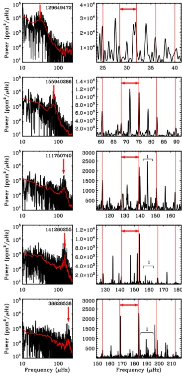
hence possibly too hot to show solar-like oscillations, or potentially contaminated. For the current test case, the number of stars was small enough that we visually checked the results, which confirmed all detections and the non-detection. The power spectra of a representative sample of the stars are shown in Figure 2, showing clear oscillation excess power and the frequency pattern required to measure bothνmaxandΔν.
The neural network also supplies a rough estimate forνmax, which we provided as a prior to 13 independent groups analyzing the power spectra to extract high-precision values of both νmax, Δν, and their respective uncertainties using their preferred method. These methods have been thoroughly tested and described in the literature(see, e.g., Gaulme et al. 2009; Huber et al. 2009; Hekker et al. 2010; Mathur et al. 2010; Mosser et al. 2011; Kallinger et al. 2012; Corsaro & De Ridder 2014; Davies et al.2016; Campante et al.2017; Zinn et al.2019).
From the 13 independent determinations of the global asteroseismic parameters we adopted as central reference value forΔν and νmaxthe results from the pipeline by Gaulme et al. (2009), as this method was on average closest to the ensemble
mean after applying a 2σ outlier rejection. Uncertainties in the global asteroseismic parameters obtained by the selected pipeline are at the 1.9% and 2.4% level for Δν and νmax, respectively. These uncertainties are of comparable magnitude to those obtained from a single campaign with the K2 mission (see the Appendix in Stello et al.2017) and about twice as large
as those extracted from 50 days of Kepler observations (see Figures 3 and 4 in Hekker et al.2012). We report the central
values and statistical uncertainties in Δν and νmax from the selected pipeline for all targets in Table1.
For each star, we take into account the scatter across the different methods by adding in quadrature the standard deviation among the central values retained after the 2σ outlier rejection procedure to the formal uncertainty reported by the selected reference method. This consolidation process yields median uncertainties of 3.9% inΔν and 2.6% in νmax, where the individual contribution arising from this systematic component to the total uncertainty is listed in Table 1. We note that we could decrease the level of uncertainties resulting from our “blind” statistical consolidation approach by for example checking the Δν and νmax results against the power spectra and/or échelle diagrams (see Figure 5 in Stello et al.
2011). However, we want to draw a realistic picture of the
uncertainties one can expect when dealing with large ensembles of stars (as expected from TESS) where detailed “boutique” analysis/checking on a star-by-star basis is not practically feasible. Hence, our quoted uncertainties are conservative, but representative for analysis of TESS red giants where several pipelines are involved.
4. Derived Stellar Properties
We have determined stellar properties for a subsample of 17 stars that had spectroscopic measurements of effective temp-erature and chemical composition available in the littemp-erature. As 65
https://heasarc.gsfc.nasa.gov/cgi-bin/tess/webtess/wtv.py
66
T’DA Data Release Notes—Data Release 3 for TESS Sectors 1+2 (https:// doi.org/10.5281/zenodo.2510028).
3
Table 1
Measured and Derived Stellar Properties of Our Targets
TIC HIP νmax Δν V Teff [Fe/H] R M Age Atmospheric Properties
(μHz) (μHz) (mag) (K) (dex) (Re) (Me) (Gyr)
13097379 114842 59.10±1.50±1.01 6.02±0.03±0.24 6.646±0.010 4634±80 0.04±0.08 8.49±0.28±0.17 1.22±0.08±0.06 6.10±1.06±0.97 Luck(2015) 38574220 19805 29.40±0.90±0.72 4.06±0.20±0.26 5.577±0.009 L L L L L L 38828538 21253 189.90±1.60±0.42 14.90±0.10±0.13 5.896±0.009 4828±80 0.11±0.08 4.66±0.10±0.06 1.21±0.05±0.03 6.20±0.50±1.02 Alves et al.(2015) 39082723 4293 49.30±2.10±1.99 5.20±0.10±0.06 5.574±0.009 4706±80 −0.05±0.08 9.30±0.27±0.17 1.19±0.09±0.07 5.90±1.20±1.37 Alves et al.(2015) 47424090 112612 28.30±1.80±1.90 3.40±0.10±0.29 6.930±0.010 L L L L L L 70797228 655 31.80±1.50±0.75 4.37±0.20±0.37 5.787±0.009 4750±80 0.12±0.08 11.27±0.61±0.47 1.19±0.13±0.11 6.80±2.20±2.20 Jones et al.(2011) 77116701 103071 48.30±7.60±29.85 5.64±0.20±3.37 8.568±0.018 L L L L L L 111750740 113148 142.60±2.70±1.11 11.80±0.10±0.23 5.658±0.009 4688±80 0.16±0.08 5.11±0.16±0.09 1.06±0.07±0.05 10.80±1.78±1.71 Wittenmyer et al.(2016) 115011683 103836 58.80±1.20±0.97 6.10±0.10±0.01 6.057±0.010 4590±80 −0.13±0.08 7.92±0.21±0.22 1.04±0.07±0.07 9.90±1.63±2.01 Wittenmyer et al.(2016) 129649472 105854 31.80±1.20±1.39 4.20±0.20±0.11 5.755±0.009 4748±80 0.28±0.08 10.85±0.60±0.24 1.13±0.12±0.06 8.50±2.76±1.87 Jofré et al.(2015) 139756492 106566 27.60±0.90±0.35 4.16±0.20±0.65 6.819±0.010 L L L L L L 141280255 25918 150.40±1.00±0.57 12.52±0.02±0.10 5.307±0.009 4630±80 0.33±0.08 4.98±0.12±0.05 1.07±0.06±0.03 11.70±2.62±2.39 Meléndez et al.(2008) 144335025 117075 68.50±1.60±0.64 7.35±0.20±0.39 6.194±0.010 L L L L L L 149347992 26190 165.80±4.10±16.12 11.10±0.40±0.60 6.405±0.010 5132±80 −0.17±0.08 7.20±0.38±0.20 2.17±0.22±0.06 0.80±0.30±0.10 Randich et al.(1999) 155940286 1766 73.20±1.30±0.32 7.40±0.02±0.11 6.810±0.010 4630±80 0.03±0.08 6.95±0.18±0.14 1.01±0.06±0.04 12.00±1.78±36.07 Wittenmyer et al.(2016) 175375523 114775 60.00±1.10±0.30 5.80±0.10±0.14 5.899±0.009 4660±80 0.26±0.08 9.00±0.30±0.58 1.38±0.09±0.21 4.50±0.76±1.35 Jones et al.(2011) 183537408 117659 57.90±1.10±0.80 6.20±0.20±0.42 6.781±0.010 L L L L L L 204313960 113801 106.00±3.30±1.47 9.40±0.50±0.43 6.083±0.010 4897±80 −0.20±0.08 6.50±0.18±0.13 1.32±0.07±0.05 3.80±0.57±0.57 Randich et al.(1999) 220517490 12871 117.30±1.20±0.60 10.87±0.02±0.15 5.846±0.009 4961±80 −0.26±0.08 5.61±0.11±0.10 1.10±0.04±0.04 6.10±0.50±1.18 Alves et al.(2015) 237914586 17440 47.00±1.40±1.33 5.74±0.20±0.08 3.959±0.009 L L L L L L 270245797 109584 72.20±1.70±0.64 6.60±0.10±0.27 6.239±0.009 4824±80 −0.10±0.08 8.73±0.23±0.39 1.60±0.09±0.13 2.10±0.22±0.64 Alves et al.(2015) 281597433 2789 73.30±1.00±1.37 7.20±0.03±0.19 6.163±0.010 4700±80 −0.41±0.08 6.77±0.15±0.24 0.95±0.05±0.08 11.00±1.35±2.73 Randich et al.(1999) 439399563 343 44.30±1.40±0.66 4.54±0.06±0.11 5.892±0.009 4778±80 0.11±0.08 10.69±0.34±0.40 1.44±0.11±0.14 3.50±0.71±0.78 da Silva et al.(2015) 441387330 102014 46.60±0.80±0.86 5.25±0.10±0.25 5.592±0.009 4710±80 −0.02±0.08 10.18±0.34±0.68 1.40±0.09±0.20 3.40±0.57±1.19 Jones et al.(2011) Note.Observed V-magnitudes are extracted from the Tycho-2 catalog. The global asteroseismic quantities and stellar properties include a statistical and systematic component derived as described in Sections3and4, respectively. We report them here as value±σsta±σsys. The last column gives the reference from which we retrieved the central values of Teffand[Fe/H] used for the grid-based modeling. Their uncertainties have
been homogenized to 80K and 0.08dex, respectively (see Section4).
(This table is available in its entirety in machine-readable form.)
4 The Astrophysical Journal Letters, 889:L34 (8pp ), 2020 February 1 Silva Aguirre et al.
one of our goals is to follow the same analysis procedure expected for large ensembles of stars, we assumed fixed uncertainties in Teff and [Fe/H] of 80K and 0.08dex, which are at the level of those provided by current large-scale spectroscopic surveys. To extract the physical properties of our sample, the atmospheric information was complemented with the asteroseismic scaling relations:
n n r r D D 1 2 ⎛ ⎝ ⎜ ⎞⎠⎟ ( ) n n -M M R R T T , 2 max max, 2 eff eff, 1 2 ⎛ ⎝ ⎜ ⎞ ⎠ ⎟ ⎛ ⎝ ⎜ ⎞⎠⎟ ⎛ ⎝ ⎜ ⎞ ⎠ ⎟ ( )
where we adoptedΔνe=135.5 (μHz) and νmax,e=3140 (μHz) as obtained by our reference pipeline from the analysis of solar data.
Seven teams independently applied grid-based modeling pipelines based on stellar evolution models or isochrones to determine the main physical properties of the targets(see Basu et al. 2012; Silva Aguirre et al.2015; Rodrigues et al. 2017; Mints & Hekker 2018; Yıldız et al. 2019, and references therein). When matching the models to the atmospheric properties and the global asteroseismic parameters Δν and νmax the pipelines yielded median uncertainties of ∼6% in radius, ∼14% in mass, and ∼50% in age. These statistical uncertainties are of the same magnitude to those obtained with the K2 mission (Sharma et al. 2019), as expected from the
similar resulting errors in the global seismic parameters described in Section 3, and about a factor of two larger than what can be achieved with the full duration of the Kepler observations(Pinsonneault et al.2018).
In addition to the asteroseismic information, five of the pipelines can include parallaxes from Gaia DR2 (Gaia Collaboration et al. 2018) coupled with Tycho-2 (Høg et al. 2000) observed V-magnitudes in their fitting algorithm to
further constrain the stellar properties. As a consequence of having the additional constraint on stellar radius from the astrometry, the resulting uncertainties decrease to a level of ∼3% in radius, ∼6% in mass, and ∼20% in age. This level of precision resembles that obtained with the use of the full length of asteroseismic observations from the nominal Kepler mission, and emphasizes the potential of TESS for Galactic studies using
Figure 1. Asteroseismic HR diagram showing (predicted) νmax instead of luminosity. Red dots show the selected targets inside the black selection box. For reference, the Sun is shown as well as all Hipparcos stars brighter than sixth magnitude(gray dots). Solar metallicity MESA tracks from Stello et al. (2013) are shown to guide the eye with masses in solar units indicated (pre- and
post- helium core-ignition phases are shown separately).
Figure 2.Power spectra sample of our targets representative of theνmaxrange that they cover from around the red clump(top) to the low luminosity red giant branch(bottom). Left panels: spectra shown in log–log space (smoothed in red) showing the location of the oscillation power excess,νmax, indicated by red arrows on top of a frequency-dependent granulation background andflat white noise component. Right panels: close-up of spectra showing locations of the roughly equally spaced radial modes(using red equally spaced vertical lines to guide the eye) and their average separation, Δν (red horizontal arrows). In the three bottom rows multiple dipole(l = 1) mixed modes are resolved in between consecutive radial modes as indicated by the black brackets.
5
red giants given its larger sky coverage, simple and reproducible selection function, and one order of magnitude higher expected yield of asteroseismic detections than any other previous mission.
To illustrate the differences in the obtained stellar properties arising from the selection offitted observables, Figure3shows the stellar radius obtained with one of the pipelines (BASTA; Silva Aguirre et al. 2015) when fitting different combinations
of input parameters. Thefigure uses as the reference value the case when, in addition to the atmospheric properties, only the Gaia DR2 parallax and observed V-band magnitude are included in the fit. For the majority of the targets the results are consistent across the three sets within their formal statistical uncertainties. A summary of the measured and derived stellar properties for our targets can be found in Table 1, where we have listed the central values and statistical uncertainties obtained with the BASTA pipeline, and determined the systematic contribution as the standard deviation across the results reported by all pipelines.
Two targets(TIC 141280255 and TIC 149347992) present a larger disagreement between the radii obtained with parallax and the seismic set(Δν, νmax). We investigated whether these discrepancies were due to the quality of the astrometric data by computing the re-normalized unit weight error (RUWE)67 for our sample of stars. In the case of TIC141280255 we obtained a RUWE= 1.98, which is above the value recommended by the Gaia team as a criterion for a good astrometric solution (RUWE1.4). Therefore, we adopt for this star the stellar properties obtained from fitting the asteroseismic input only (Δν, νmax).
In the case of TIC149347992 the discrepancy is the result of predicted evolutionary phases: while the parallax-only solution suggests that the star in the clump phase, the asteroseismic fit favors a star in the red giant branch. The combinedfit therefore presents a bimodal distribution that encompasses these two families of solutions. A similar situation occurs in the fit of TIC175375523, which shows agreement in the radius
determined from different sets of input but has a fractional age uncertainty above unity when only(Δν, νmax) are included in thefit. Its resulting age distribution is bimodal in this set as both red giant branch and clump models can reproduce the observations, but the inclusion of parallax information favors the red giant branch solution and accounts for the ∼17% statistical uncertainty reported in Table 1. The availability of evolutionary classifications from deep neural networks trained on short Kepler data(Hon et al.2018) would further decrease
the obtained uncertainties by clearly disentangling these two scenarios.
In Figure 4 we plot the distribution of fractional age uncertainties obtained with BASTA for the three considered cases of input, showing the clear improvement in precision when asteroseismic information and parallax are simulta-neously included in thefit. For visualization purposes we have excluded the target TIC175375523 from the figure. Our stellar ages at the 20% level are significantly more precise than what is obtained by data-driven and neural-network methods trained using asteroseismic ages from Kepler(above the 30% level, see e.g., Mackereth et al. 2019). As a final remark, we note that
asteroseismically derived properties of red giants are accurate to at least a similar level than our statistical uncertainties (below ∼5% and ∼10% for radii and masses, respectively; see the discussion in e.g., Pinsonneault et al.2018, and references therein). We have made emphasis on our achieved precision instead of accuracy as our results could still be affected by a systematic component arising from uncertainties in evolution-ary calculations, although recent investigations quantifying these effects at solar metallicity suggest that they are smaller than our statistical uncertainties(Silva Aguirre et al.2019).
5. Conclusions
We presented the first ensemble analysis of red giant stars observed with the TESS mission. We selected a sample of 25 stars where we expected to detect oscillations based on their magnitude and parallax value, and analyzed the extracted light curves in search for asteroseismic signatures in the power spectra. Our mainfindings can be summarized as follows.
Figure 3. Comparison of stellar radii obtained with BASTA when fitting different combinations of input parameters: Gaia DR2 parallax and V-band magnitude(ϖ), global asteroseismic parameters (Δν,νmax), and all combined (ϖ,Δν,νmax). Effective temperature and composition are also fitted in all cases. See the text for details.
Figure 4.Distribution of fractional age uncertainties for our sample of stars determined by theBASTA pipeline fitting different combinations of available observables. The points indicate the individual values used to construct the Gaussian kernel density estimation. For better visualization we have excluded TIC175375523 from the figure. See the text for details.
67
See Gaia technical note GAIA-C3-TN-LU-LL-124-01 (https://www.
cosmos.esa.int/web/gaia/dr2-known-issues).
1. We detected oscillations in all the stars(except one that was likely incorrectly listed as a red giant). Despite the modest number of stars in our sample, our detection yield supports that the TESS photometric performance is similar to that of Kepler and K2 except shifted by about 5 magnitudes toward brighter stars due to its smaller aperture.
2. Individual pipelines retrieve the global asteroseismic parameters with uncertainties at the∼2% level in Δν and ∼2.5% in νmax, which, respectively, increase to∼4% and ∼3.5% when we take into account the scatter across results. We consider these uncertainties to be representa-tive for the forthcoming ensemble analysis of TESS targets observed in 1–2 sectors, as individual validation of the results will not be feasible due to the large number of targets observed.
3. Grid-based modeling techniques applying asteroseismic scaling relations were used to retrieve stellar properties for the 17 targets with spectroscopic information. Radii, masses, and ages were obtained with uncertainties at the 6%, 14%, and 50% level, and decrease to 3%, 6%, and 20% when parallax information from Gaia DR2 is included.
The expected number of red giants with detected oscillations by TESS (∼500,00068) greatly surpasses the final yield of Kepler (∼20,000). In this respect, the combination of TESS observations, Gaia astrometry, and large-scale spectroscopic surveys holds a great potential for studies of Galactic structure where precise stellar properties (particularly ages) are of key importance. We note that the recently approved extended TESS mission will change the 30 minutes cadence to 10 minutes, making it possible to detect oscillations of stars of smaller radii using the full-frame images. This will enable more rigorous investigations of the asteroseismic mass scale for giants when anchored to empirical mass determinations(e.g., from eclipsing binaries) of turn-off and subgiant stars.
This Letter includes data collected by the TESS mission, which are publicly available from the Mikulski Archive for Space Telescopes (MAST). Funding for the TESS mission is provided by NASAʼs Science Mission directorate. Funding for the TESS Asteroseismic Science Operations Centre is provided by the Danish National Research Foundation(grant agreement
No. DNRF106), ESA PRODEX (PEA 4000119301), and
Stellar Astrophysics Centre(SAC) at Aarhus University. V.S. A. acknowledges support from the Independent Research Fund Denmark(Research grant 7027-00096B). D.B. is supported in the form of work contract FCT/MCTES through national funds and by FEDER through COMPETE2020 in connection to these grants: UID/FIS/04434/2019; PTDC/FIS-AST/30389/2017 & POCI-01-0145-FEDER-030389. L.B., R.A.G., and B.M. acknowledge the support from the CNES/PLATO grant. D.B. acknowledges NASA grant NNX16AB76G. T.L.C. acknowl-edges support from the European Union’s Horizon 2020 research and innovation programme under the Marie Sk ło-dowska-Curie grant agreement No.792848 (PULSATION). This work was supported by FCT/MCTES through national funds(UID/FIS/04434/2019). E.C. is funded by the European Unionʼs Horizon 2020 research and innovation program under
the Marie Skłodowska-Curie grant agreement No. 664931. R.H. and M.N.L. acknowledge the support of the ESA PRODEX programme. T.S.R. acknowledges financial support from Premiale 2015 MITiC(PI B. Garilli). K.J.B. is supported by the National Science Foundation under Award AST-1903828. M. S.L. is supported by the Carlsberg Foundation (grant agreement No. CF17-0760). M.C. is funded by FCT//MCTES through national funds and by FEDER through COMPETE2020 through these grants: UID/FIS/04434/2019, PTDC/FIS-AST/30389/ 2017 & POCI-01-0145-FEDER-030389, CEECIND/02619/ 2017. The research leading to the presented results has received funding from the European Research Council under the European Community’s Seventh Framework Programme (FP7/2007-2013)/ ERC grant agreement no 338251 (StellarAges). A.M. acknowl-edges support from the European Research Council Consolidator
Grant funding scheme (project ASTEROCHRONOMETRY,
grant agreement No. 772293,http://www.asterochronometry.eu).
A.M.S. is partially supported by MINECO grant ESP2017-82674-R. J.C.S. acknowledges funding support from Spanish public funds for research under projects ESP2017-87676-2-2, and from project RYC-2012-09913 under the ‘Ramón y Cajal’ program of the Spanish Ministry of Science and Education. Resources supporting this work were provided by the NASA
High-End Computing (HEC) Program through the NASA
Advanced Supercomputing (NAS) Division at Ames Research Center for the production of the SPOC data products.
ORCID iDs
Víctor Silva Aguirre https: //orcid.org/0000-0002-6137-903X
Dennis Stello https://orcid.org/0000-0002-4879-3519
Amalie Stokholm https://orcid.org/0000-0002-5496-365X
Jakob R. Mosumgaard https: //orcid.org/0000-0001-9234-430X
Warrick H. Ball https://orcid.org/0000-0002-4773-1017
Sarbani Basu https://orcid.org/0000-0002-6163-3472
Diego Bossini https://orcid.org/0000-0002-9480-8400
Lisa Bugnet https://orcid.org/0000-0003-0142-4000
Derek Buzasi https://orcid.org/0000-0002-1988-143X
Tiago L. Campante https://orcid.org/0000-0002-4588-5389
Lindsey Carboneau https://orcid.org/0000-0003-1001-5137
William J. Chaplin https://orcid.org/0000-0002-5714-8618
Enrico Corsaro https://orcid.org/0000-0001-8835-2075
Guy R. Davies https://orcid.org/0000-0002-4290-7351
Rafael A. García https://orcid.org/0000-0002-8854-3776
Patrick Gaulme https://orcid.org/0000-0001-8330-5464
Oliver J. Hall https://orcid.org/0000-0002-0468-4775
Rasmus Handberg https://orcid.org/0000-0001-8725-4502
Marc Hon https://orcid.org/0000-0003-2400-6960
Thomas Kallinger https://orcid.org/0000-0003-3627-2561
Liu Kang https://orcid.org/0000-0001-5219-7894
Mikkel N. Lund https://orcid.org/0000-0001-9214-5642
Savita Mathur https://orcid.org/0000-0002-0129-0316
Alexey Mints https://orcid.org/0000-0002-8440-1455
Benoit Mosser https://orcid.org/0000-0002-7547-1208
Zeynep Çelik Orhan https: //orcid.org/0000-0002-9424-2339
Thaíse S. Rodrigues https: //orcid.org/0000-0002-9414-339X
Mutlu Yıldız https://orcid.org/0000-0002-7772-7641
Joel C. Zinn https://orcid.org/0000-0002-7550-7151
Sibel Örtel https://orcid.org/0000-0001-5759-7790
68Based on a preliminary simulation of the full TESS sky(TESS GI Proposal No. G011188).
7
Paul G. Beck https://orcid.org/0000-0003-4745-2242
Keaton J. Bell https://orcid.org/0000-0002-0656-032X
Zhao Guo https://orcid.org/0000-0002-0951-2171
Chen Jiang https://orcid.org/0000-0002-7614-1665
James S. Kuszlewicz https://orcid.org/0000-0002-3322-5279
Marc Pinsonneault https://orcid.org/0000-0002-7549-7766
Jamie Tayar https://orcid.org/0000-0002-4818-7885
Margarida S. Cunha https: //orcid.org/0000-0001-8237-7343
Saskia Hekker https://orcid.org/0000-0002-1463-726X
Andrea Miglio https://orcid.org/0000-0001-5998-8533
Mario J. P. F. G. Monteiro https: //orcid.org/0000-0003-0513-8116
Ditte Slumstrup https://orcid.org/0000-0003-4538-9518
George Angelou https://orcid.org/0000-0003-4463-1907
Othman Benomar https://orcid.org/0000-0001-9405-5552
Aliz Derekas https://orcid.org/0000-0002-6526-9444
Maria Pia Di Mauro https://orcid.org/0000-0001-7801-7484
Yveline Lebreton https://orcid.org/0000-0002-4834-2144
Jaymie Matthews https://orcid.org/0000-0002-4461-080X
Nicolas Nardetto https://orcid.org/0000-0002-7399-0231
Jose D. do Nascimento, Jr. https: //orcid.org/0000-0001-7804-2145
Filipe Pereira https://orcid.org/0000-0002-2157-7146
Luisa F. Rodríguez Díaz https: //orcid.org/0000-0002-0588-1375
Emanuele Spitoni https://orcid.org/0000-0001-9715-5727
Vincent Van Eylen https://orcid.org/0000-0001-5542-8870
Rita Ventura https://orcid.org/0000-0002-5152-0482
Kuldeep Verma https://orcid.org/0000-0003-0970-6440
Achim Weiss https://orcid.org/0000-0002-3843-1653
Tao Wu https://orcid.org/0000-0001-6832-4325
Thomas Barclay https://orcid.org/0000-0001-7139-2724
Jørgen Christensen-Dalsgaard https: //orcid.org/0000-0001-5137-0966
Jon M. Jenkins https://orcid.org/0000-0002-4715-9460
Sara Seager https://orcid.org/0000-0002-6892-6948
Roland Vanderspek https://orcid.org/0000-0001-6763-6562
References
Alves, S., Benamati, L., Santos, N. C., et al. 2015,MNRAS,448, 2749
Anders, F., Chiappini, C., Rodrigues, T. S., et al. 2017,A&A,597, A30
Basu, S., Verner, G. A., Chaplin, W. J., & Elsworth, Y. 2012,ApJ,746, 76
Bedding, T. R., Huber, D., Stello, D., et al. 2010,ApJL,713, L176
Bedding, T. R., Mosser, B., Huber, D., et al. 2011,Natur,471, 608
Campante, T. L., Corsaro, E., Lund, M. N., et al. 2019,ApJ,885, 31
Campante, T. L., Veras, D., North, T. S. H., et al. 2017,MNRAS,469, 1360
Casagrande, L., Silva Aguirre, V., Schlesinger, K. J., et al. 2016,MNRAS,
455, 987
Corsaro, E., & De Ridder, J. 2014,A&A,571, A71
da Silva, R., Milone, A. d. C., & Rocha-Pinto, H. J. 2015,A&A,580, A24
Davies, G. R., Silva Aguirre, V., Bedding, T. R., et al. 2016, MNRAS,
456, 2183
Flower, P. J. 1996,ApJ,469, 355
Gaia Collaboration, Katz, D., Antoja, T., et al. 2018,A&A,616, A11
Gaulme, P., Appourchaux, T., & Boumier, P. 2009,A&A,506, 7
Handberg, R., & Lund, M. N. 2014,MNRAS,445, 2698
Hekker, S., Broomhall, A.-M., Chaplin, W. J., et al. 2010, MNRAS, 402, 2049
Hekker, S., Elsworth, Y., Mosser, B., et al. 2012,A&A,544, A90
Høg, E., Fabricius, C., Makarov, V. V., et al. 2000, A&A,355, L27
Hon, M., Stello, D., & Yu, J. 2018,MNRAS,476, 3233
Houk, N. 1994, in ASP Conf. Ser. 60, The MK Process at 50 years: A Powerful Tool for Astrophysical Insight, ed. C. Corbally, R. O. Gray, & R. F. Garrison(San Francisco, CA: ASP),285
Huber, D., Stello, D., Bedding, T. R., et al. 2009, CoAst,160, 74
Jenkins, J. M., Twicken, J. D., McCauliff, S., et al. 2016,Proc. SPIE,9913, 99133E
Jofré, E., Petrucci, R., Saffe, C., et al. 2015,A&A,574, A50
Jones, M. I., Jenkins, J. S., Rojo, P., & Melo, C. H. F. 2011,A&A,536, A71
Kallinger, T., Hekker, S., Mosser, B., et al. 2012,A&A,541, 51
Luck, R. E. 2015,AJ,150, 88
Lund, M. N., Handberg, R., Davies, G. R., Chaplin, W. J., & Jones, C. D. 2015,ApJ,806, 30
Mackereth, J. T., Bovy, J., Leung, H. W., et al. 2019,MNRAS,489, 176
Mathur, S., García, R. A., Régulo, C., et al. 2010,A&A,511, 46
Meléndez, J., Asplund, M., Alves-Brito, A., et al. 2008,A&A,484, L21
Miglio, A., Chiappini, C., Morel, T., et al. 2013,MNRAS,429, 423
Miglio, A., Montalbán, J., Baudin, F., et al. 2009,A&A,503, L21
Mints, A., & Hekker, S. 2018,A&A,618, A54
Mosser, B., Elsworth, Y., Hekker, S., et al. 2011,A&A,537, A30
Pinsonneault, M. H., Elsworth, Y. P., Tayar, J., et al. 2018,ApJS,239, 32
Randich, S., Gratton, R., Pallavicini, R., Pasquini, L., & Carretta, E. 1999, A&A,348, 487
Ricker, G. R., Winn, J. N., Vanderspek, R., et al. 2015,JATIS,1, 014003
Rodrigues, T. S., Bossini, D., Miglio, A., et al. 2017,MNRAS,467, 1433
Sharma, S., Stello, D., Bland-Hawthorn, J., et al. 2019,MNRAS,490, 5335
Silva Aguirre, V., Bojsen-Hansen, M., Slumstrup, D., et al. 2018,MNRAS,
475, 5487
Silva Aguirre, V., Christensen-Dalsgaard, J., Cassisi, S., et al. 2019, arXiv:1912.04909
Silva Aguirre, V., Davies, G. R., Basu, S., et al. 2015,MNRAS,452, 2127
Stello, D., Huber, D., Bedding, T. R., et al. 2013,ApJL,765, L41
Stello, D., Meibom, S., Gilliland, R. L., et al. 2011,ApJ,739, 13
Stello, D., Zinn, J., Elsworth, Y., et al. 2017,ApJ,835, 83
Van Leeuwen, F. 2007,A&A,474, 653
Wittenmyer, R. A., Liu, F., Wang, L., et al. 2016,AJ,152, 19
Yıldız, M., Çelik Orhan, Z., & Kayhan, C. 2019,MNRAS,489, 1753
Yu, J., Huber, D., Bedding, T. R., et al. 2018,ApJS,236, 42
Zinn, J. C., Stello, D., Huber, D., & Sharma, S. 2019,ApJ,884, 107