HAL Id: obspm-02190209
https://hal-obspm.ccsd.cnrs.fr/obspm-02190209
Submitted on 5 Nov 2020
HAL is a multi-disciplinary open access
archive for the deposit and dissemination of
sci-entific research documents, whether they are
pub-lished or not. The documents may come from
teaching and research institutions in France or
abroad, or from public or private research centers.
L’archive ouverte pluridisciplinaire HAL, est
destinée au dépôt et à la diffusion de documents
scientifiques de niveau recherche, publiés ou non,
émanant des établissements d’enseignement et de
recherche français ou étrangers, des laboratoires
publics ou privés.
Period spacings in red giants
B. Mosser, C. Pinçon, Kevin Belkacem, M. Vrard, M. Takata
To cite this version:
B. Mosser, C. Pinçon, Kevin Belkacem, M. Vrard, M. Takata. Period spacings in red giants: III.
Coupling factors of mixed modes. Astronomy and Astrophysics - A&A, EDP Sciences, 2017, 600,
pp.A1. �10.1051/0004-6361/201630053�. �obspm-02190209�
A&A 600, A1 (2017) DOI:10.1051/0004-6361/201630053 c ESO 2017
Astronomy
&
Astrophysics
Period spacings in red giants
III. Coupling factors of mixed modes
B. Mosser
1, C. Pinçon
1, K. Belkacem
1, M. Takata
2, and M. Vrard
31 LESIA, Observatoire de Paris, PSL Research University, CNRS, Université Pierre et Marie Curie, Université Paris Diderot,
92195 Meudon Cedex, France e-mail: [email protected]
2 Department of Astronomy, School of Science, The University of Tokyo, 7-3-1 Hongo, Bunkyo-ku, 113-0033 Tokyo, Japan 3 Instituto de Astrofísica e Ciências do Espaço, Universidade do Porto, CAUP, Rua das Estrelas, 4150-762 Porto, Portugal
Received 14 November 2016/ Accepted 23 December 2016
ABSTRACT
Context.The power of asteroseismology relies on the capability of global oscillations to infer the stellar structure. For evolved stars, we benefit from unique information directly carried out by mixed modes that probe their radiative cores. This third article of the series devoted to mixed modes in red giants focuses on their coupling factors, which have remained largely unexploited up to now.
Aims.With the measurement of coupling factors, we intend to give physical constraints on the regions surrounding the radiative core and the hydrogen-burning shell of subgiants and red giants.
Methods.A new method for measuring the coupling factor of mixed modes was implemented, which was derived from the method recently implemented for measuring period spacings. This new method was automated so that it could be applied to a large sample of stars.
Results.Coupling factors of mixed modes were measured for thousands of red giants. They show specific variation with mass and evolutionary stage. Weak coupling is observed for the most evolved stars on the red giant branch only; large coupling factors are measured at the transition between subgiants and red giants as well as in the red clump.
Conclusions.The measurement of coupling factors in dipole mixed modes provides a new insight into the inner interior structure of evolved stars. While the large frequency separation and the asymptotic period spacings probe the envelope and core, respectively, the coupling factor is directly sensitive to the intermediate region in between and helps determine its extent. Observationally, the determination of the coupling factor is a prior to precise fits of the mixed-mode pattern and can now be used to address further properties of the mixed-mode pattern, such as the signature of buoyancy glitches and core rotation.
Key words. stars: oscillations – stars: interiors – stars: evolution
1. Introduction
The seismic observations of large sets of stars with the CoRoT and Kepler missions, from the main sequence (Chaplin et al. 2011) up to the red giant branch (De Ridder et al. 2009), has mo-tivated intense work in stellar physics, which includes ensemble asteroseismology (e.g.,Kallinger et al. 2010;Mosser et al. 2010; Huber et al. 2011; Silva Aguirre et al. 2011; Kallinger et al. 2014). Ensemble asteroseismology is efficient for evolved stars because they host mixed modes that behave as gravity modes in the core and pressure modes in the envelope. These modes directly probe the stellar core and, therefore, reveal unique information.
Contrary to pressure modes, evenly spaced in frequency, and to gravity modes, evenly spaced in period, mixed modes show a more complicated frequency pattern. Since, for red giants, the density of gravity modes is large compared to the density of pres-sure modes, the mixed-mode pattern resembles a pure gravity-mode pattern perturbed by the pressure-gravity-mode pattern. The period spacings are close to the asymptotic value for gravity-dominated mixed modes, but are significantly smaller near expected pure pressure modes (e.g., Mosser et al. 2015). Pressure-dominated mixed modes have lower inertia than gravity-dominated mixed
modes; hence, the former show larger amplitudes (Dupret et al. 2009;Grosjean et al. 2014). Even with period spacings far from the asymptotic values, mixed modes allowed us in a first step to distinguish stars with hydrogen-burning shell from stars with core helium-burning (Bedding et al. 2011;Mosser et al. 2011a). In a second step, the asymptotic analysis of the mixed-mode pattern allowed us to derive precise information on the Brunt-Väisälä frequency profile in the radiative core (Mosser et al. 2012b). Indeed, the asymptotic expansion (Shibahashi 1979; Unno et al. 1989; Mosser et al. 2012b; Takata 2016) is a pow-erful tool for investigating mixed modes in red giants observed by the space missions CoRoT and Kepler, despite the fact that observations are not conducted in an asymptotic regime. Ob-served radial pressure orders are small; in fact, they are too small to lie in the asymptotic regime, as shown by CoRoT obser-vations (e.g., De Ridder et al. 2009; Mosser et al. 2010). How-ever,Mosser et al.(2013b) have demonstrated that the second-order asymptotic expansion provides a coherent view on the pressure mode pattern, even for the most evolved red giants (Mosser et al. 2013a). Conversely, high radial gravity orders are observed in mixed modes, except in subgiants, so that consider-ing a first-order expansion for the gravity contribution is relevant (Mosser et al. 2014).
This work allowed us to measure asymptotic period spac-ings and to derive unique information on stellar evolution. The contraction of the helium core of hydrogen-shell-burning red gi-ants is marked by the decrease of the asymptotic period spacing. Moreover, stars with a degenerate helium core (with a mass in-ferior to about 1.8 M ) on the red giant branch (RGB) show a close relationship between the large separation and period spac-ing, which is the seismic signature of the mirror effect between the core and envelope structures. In the red clump, contrary to more massive stars, core-helium burning stars with a mass lower than about 1.8 M show a tight mass-dependent relation between the asymptotic large separation and period spacing.
The use of the mixed modes for assessing the inner interior structure of red giants is, however, still in its infancy. Up to now, only the period spacings have benefitted from large-scale measurements (Vrard et al. 2016). Another important parameter, the coupling factor q, was precisely determined for just a hand-ful of stars (Buysschaert et al. 2016). This parameter benefitted from a recent breakthrough sinceTakata(2016) could derive an asymptotic expression for dipole modes using the JWKB method (Jeffreys, Wentzel, Kramers, and Brillouin), taking the perturba-tion of the gravitaperturba-tional potential into account; but this investi-gation did not use the weak-coupling approximation, contrary to the previous work byUnno et al.(1989).
Here, we use the method developed byMosser et al.(2015, Paper I of the series) to complete the large-scale analysis of Vrard et al.(2016, Paper II of the series). We specifically address the measurement of the coupling factor q of mixed modes. This parameter plays an important role in the asymptotic expansion: it expresses the link between the pressure and gravity contribu-tions to the mixed mode, which is expressed by their phases θp and θg, respectively. FollowingUnno et al.(1989), the asymp-totic expansion is written
tan θp= q tan θg, (1)
with the phases defined as
θg = π 1 ∆Π1 1 ν − 1 νg ! , (2) θp = π ν − νp ∆νp , (3)
where νpand νgare the asymptotic frequencies of pure pressure and gravity modes, respectively, and∆νpis the frequency di ffer-ence between the consecutive pure pressure radial modes with radial orders npand np+ 1, as defined byMosser et al.(2015).
While θp and θgaccount for the propagation of the wave in the envelope and core, respectively, the coupling factor comes from the contribution of the region between the Brunt-Väisälä cavity and the Lamb profile S`=
√
`(` + 1) c/r, where the oscil-lation is evanescent. Hence, studying the coupling factor q pro-vides a direct way to examine the evanescent region, namely the physical regions surrounding the hydrogen-burning shell, where most of the stellar luminosity is produced. This param-eter also plays a crucial role in examining rotational splittings (Goupil et al. 2013;Deheuvels et al. 2015) and mode visibilities (Mosser et al. 2017), so that its thorough examination becomes crucial in red giant seismology.
The article is organized as follows. Section2 presents the framework of our analysis. We use the weak-coupling cases to illustrate and emphasize how q is linked to stellar interior prop-erties. We also introduce the strong-coupling case, which is nec-essary at various evolutionary stages. In Sect.3, we develop a
Fig. 1.Brunt-Väisälä and Lamb frequency profiles for a 1.3-M
stel-lar model on the RGB, corresponding to model M1 ofBelkacem et al.
(2015, see also Table3). The horizontal dashed lines delimit the fre-quency range in which oscillations are expected, around νmax; the
verti-cal dotted lines indicate the locations of the hydrogen-burning shell and base of the convection zone (BCZ), respectively.
specific method for measuring the coupling factors in an auto-mated way. Section4 presents the results derived from the set of Kepler red giants analyzed byVrard et al.(2016). The results are discussed in Sect.5.
2. Coupling factor of mixed modes
In this section, we show how the coupling factor of mixed modes can be used to probe the stellar interior. We restrain the analysis to dipole mixed modes (`= 1).
2.1. Evanescent region
The coupling factor in Eq. (1) measures the decay of the wave in the region between the cavities delimited by the Brunt-Väisälä frequency NBV and the Lamb frequency S1 (Fig.1). This in-termediate zone is called the evanescent region. In the JWKB approximation, thus assuming that the wavelength of the oscil-lations is much shorter than the scale height of the equilibrium stellar structure, the radial component of the wave vector κ in the evanescent region can be written
κ = q (S2 1−ω2)(ω2− N 2 BV) cω , (4)
where c is the sound speed and ω is the angular frequency. We assume in the following that the evanescent zone is lo-cated between the hydrogen-burning shell and the base of the convective envelope. The Brunt-Väisälä and Lamb frequencies show similar radial variations in this region probed by the mixed modes (Fig.1 and, e.g., Fig. 2 ofMontalbán et al. 2012). Both can be approximated with a power law with similar exponent, −dln NBV
dln r = βN'β ' βS = − dln S1
dln r · (5)
In fact, the exponent β measures the density contrast between the core and the envelope: the higher the contrast, the higher β. We expect β to increase with the evolution and contraction of the core. In evolved red giants, where the density contrast between the envelope and the core is high enough to ensure that the local
B. Mosser et al.: Coupling factors of mixed mode
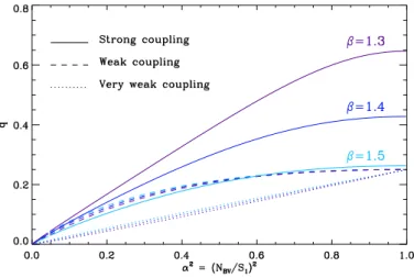
Fig. 2.Relationship between the coupling factor q and the ratio α2 =
(NBV/S1)2 defined under the assumption that both frequencies have
the same slope varying as r−βin the region surrounding the hydrogen-burning shell; q is computed for three different values of β (1.3, 1.4, and 1.5) in three cases: very weak (dotted lines, Eqs. (10), (11)), weak (dashed lines, Eqs. (7)–(9)), or strong coupling (full lines, Eqs. (12)– (14)). The very weak and weak coupling values hardly depend on β, unlike the strong-coupling case.
gravity varies as r−2in the evanescent region, β is expected to be close to the upper limit of 3/2 (Takata 2016).
As a consequence of the parallel variations of NBVand S1, the ratio
α = NBV/S1 (6)
can be considered as nearly uniform in the region above the hydrogen-burning shell where the oscillation is evanescent. A very thin evanescent zone means α is close to unity, whereas a wide one has a small α. In the following, we use this ratio α as a measure of the extent of the evanescent region and aim at linking α and β with q.
2.2. Weak coupling
In the case of weak coupling, the decay of the wave amplitude in the evanescent region E is expressed by the transmission factor defined as T ≡exp − Z E κ dr ! , (7)
which is linked to the coupling factor q of the asymptotic expan-sion (Eq. (1)) by
q=T 2
4 , (8)
as computed byShibahashi(1979) andUnno et al.(1989). Weak coupling is ensured if the transition region between S1 and NBVis wide enough. Indeed, as shown by Eqs. (7) and (8), the value of q in the case of weak coupling is necessarily below 1/4. Conversely, a value of q above 1/4 implies that the weak-coupling approach is insufficient.
With the assumptions made in Sect.2.1, so with the defini-tions of α (Eq. (6)) and β (Eq. (5)), the integral term in Eq. (7) can be rewritten Z E κ dr = √ 2 β Z 1 α √ 1 − x2 √ x2−α2 dx x2, (9)
where x is the normalized frequency ω/S1. Consequently, the coupling factor only depends on α and β, but does not vary in the frequency range in which modes are observed. Although the evanescent region is probed at different depths by the different mixed modes, the wave transmissions through the barrier, hence q, are the same for each frequency because of the parallel varia-tions of NBVand S1. This result confirms that q is directly related to the interior structure properties (Fig.2).
In the case of very weak coupling, the influence of the turn-ing points can be neglected in Eq. (7). In practice, we consider that S1 ω NBValmost everywhere between the boundaries of the evanescent region r1and r2, so that q reduces to a simple function of these boundaries
q ' 1 4 r1 r2 !2 √ 2 · (10)
Combined with the assumption on the variations of NBVand S1, it can be rewritten in terms of the coefficients α and β as follows:
q ' 1 4 α
2√2/β. (11)
This simplified relation shows again that q does not vary in the frequency range in which mixed modes are observed. It also proves that q provides another diagnostic parameter of red gi-ants, complementary to the period spacing∆Π1 that probes the Brunt-Väisälä cavity.
2.3. Strong coupling
In the strong coupling case studied byTakata(2016), the expres-sion of the transmisexpres-sion T is not as simple as Eq. (7) and must be replaced by a more precise expression. The relation between qand T becomes
T2= 4q
(1+ q)2· (12)
The factor q is connected to interior structure properties in the general case
q=1 − p1 − exp(−2πX)
1+ p1 − exp(−2πX), (13)
following Eq. (133) of Takata(2016). The new variable X de-fined by Eq. (61) of this paper expresses
X ∝ Z
E
κ dr + XR, (14)
where the additional term XR is only important when the fre-quencies NBV and S1 are very close to each other. This term comes from the gradient of NBVand S1in the evanescent region. In practice, XRtakes the reflection of the wave at the boundaries into account and thereby explains that the transmission cannot be equal to unity even when NBVand S1have very close values. As a result, a very narrow evanescent region characterized by α ' 1 is not associated with a coupling factor close to one.
The variation of X and the relation between X and q make it possible to have values of q significantly above the limit of 1/4 fixed by the weak-coupling case (Eq. (8)). Under the assumption that NBVand S1show similar radial variations, the computation of X, hence q, depends only on α and β. The variations of q with α2are shown in Fig.2, computed with Eq. (A80) ofTakata A1, page 3 of10
(2016). This equation takes into account the perturbation of the gravitational potential that modifies the values of NBV and S1. The comparison of the weak and strong coupling also shows that the use of the weak-coupling case is relevant for very low values of q only.
We note that, the lower the β, the larger the correction on q in the strong-coupling case. Moreover, the observations of q values larger than 1/4 are associated with β values of less than 1.5. Also, the correction increases when α increases.
As in the weak-coupling case, q does not show variation in the frequency range in which modes are observed. This is the consequence of parallel variations of NBVand S1. In the follow-ing, we consider that the variation of q with frequency is small enough, so that fitting the whole mixed-mode spectrum with a fixed coupling factor makes sense.
3. Method
In previous work (Mosser et al. 2012b,2014), coupling factors in red giants were derived from the fit of the oscillation pattern. This fitting method, even if made precise and easy with the new view exposed inMosser et al.(2015), cannot be automated and, therefore, we have to provide a new method for dealing with the amount of Kepler data.
3.1. Correlations between mixed-mode parameters
The method ofVrard et al.(2016) developed for measuring the period spacing∆Π1offers an efficient basis for obtaining a rel-evant measure of q. According to Eq. (1), the measurements of the mixed-mode parameters q and∆Π1are a priori independent: ∆Π1 measures the period spacings between the mixed modes whereas q measures the deformation of these spacings close to the pure pressure modes (see, e.g., Fig. 2 ofVrard et al. 2016). When buoyancy glitches, rotational splittings, or simply noise, locally modify the frequency interval between two consecutive mixed modes; this independence is however not ensured. In fact, buoyancy glitches introduce a crosstalk between the determina-tion of q and∆Π1, which induces spurious fluctuations of q when computing∆Π1.Vrard et al.(2016), who considered q a free pa-rameter when measuring period spacings∆Π1, obtained q with large uncertainties. In order to get q in a robust manner, we first had to circumvent this crosstalk. To do so, we chose to measure qand∆Π1in an independent manner. For measuring q, we con-sidered first ∆Π1 as a fixed parameter, adopting the values of Vrard et al.(2016).
3.2. Measuring q
In practice, the first step of the method consists in a stretching of the power spectrum P(ν) by using the change of variable in-troduced byMosser et al.(2015). The frequency ν is replaced by the stretched period τ according to
dτ=1 ζ
dν
ν2, (15)
where the function ζ is obtained from the interpolation of the values obtained for the dipole mixed-mode frequencies νm, ζ(νm)= " 1+1 q ν2 m∆Π1 ∆νp cos2θ g cos2θ p #−1 · (16)
The way to obtain a precise continuous function of ζ is ex-plained by Mosser et al.(2015). It importantly depends on the
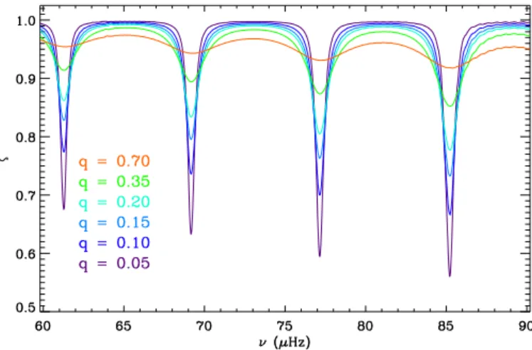
Fig. 3.Variation of the stretching function ζ with q. The locations of the local minima of ζ, which correspond to the expected pure pressure modes, do not depend on the value of q.
Fig. 4.Variation of the signal Q with the coupling factor qtestused in the
stretching function ζ considered as a free parameter, for a typical clump star (KIC 1717994). The region with maximum Q values (full symbols) is used to define the optimum value of q and the associated uncertainty δq. The dotted lines delimit the range q ± δq.
correct location of the pure dipole modes, which is carried out by the use of the red giant universal pattern (Mosser et al. 2011b; Corsaro et al. 2012).
The power spectrum P(τ) expressed as a function of the stretched period τ is composed of M blended comb-like pat-terns, where M is the number of visible azimuthal orders. For a star seen equator-on, M= 2, only 1 when the star is seen pole-on, and 3 in the intermediate case.
The regularity of the M comb(s) is optimized when the value of ζ used for stretching the spectrum matches the correct cou-pling (Fig.3). So, we varied the coupling factor qtestto obtain a varying correction ζ and searched to optimize the regularity of the comb. The optimum signal is inferred from the maximum of the Fourier transform of P(τ), noted Q (Fig.4). As is clear from Fig.3, the regularization is only slightly affected by q, so that the measurement is only possible for high signal-to-noise spectra.
3.3. Individual check and limitations
The robustness of the method was verified with individual checks based on typical red giant oscillation spectra observed
B. Mosser et al.: Coupling factors of mixed mode at various evolutionary stages. This check first allowed us to
verify that more than 96% of the prior values of∆Π1 automat-ically measured by Vrard et al. (2016) are safe. Wrong initial values of ∆Π1 were identified by spurious measures of q. For oscillation spectra with a low signal-to-noise ratio, measuring the period spacing ∆Π1 still remains possible, but identifying the small variations due to the coupling is demanding. For high signal-to-noise ratio oscillation spectra, we identified three ma-jor cases providing us with incorrect measurements for q: pres-sure glitches, buoyancy glitches, and rotation. All these effects perturb the regularity of the function ζ.
3.3.1. Pressure glitches
Pressure glitches occur when rapid variations of the sound speed modify the regularity of pressure modes. They contribute by adding a small modulation to the pressure mode pattern. The shift remains less than 2% of∆ν, as measured in the radial modes of a large set of red giants byVrard et al.(2015). The modula-tion of the pure dipole pressure modes is similar to that of radial modes, so that the location of pressure-dominated mixed modes are shifted. As a result, the local minima of the stretching func-tion ζ are shifted (Fig. 7 ofMosser et al. 2015). This change may induce a spurious variation of Q, so that the method fails. More importantly, the method often produced very low or very large spurious values of q in that case.
3.3.2. Buoyancy glitches
Buoyancy glitches occur when rapid variations of the Brunt-Väisälä frequency modify the regularity of the gravity-mode pattern. This effect was theoretically investigated by Cunha et al.(2015); it affects mixed modes since it locally mod-ifies the period of the stretched spectrum, with a clear signature on the function ζ (Figs. 8 and 10 ofMosser et al. 2015). Measur-ing a mean period spacMeasur-ing in the presence of buoyancy glitches is often possible, but measuring its optimization for deriving q is more challenging, since variations of the period spacings due to the buoyancy glitch mimic variations because of an inadequate value of q. This situation most often occurs for red clump stars and may explain part of the large spread of q observed for these stars.
3.3.3. Rotational splittings
Rotational splittings also perturb the measurements of q. In the case of low rotation (Mosser et al. 2012a), each family of stretched peaks associated with a given azimuthal order m pro-vides a comb spectrum with a period close to ∆Π1 (Fig. 6 of Mosser et al. 2015), so that the identification of ∆Π1 and of q is clearly derived from the optimization of the Fourier analy-sis of P(τ). However, the signature of the period spacings be-tween the different peaks with different azimuthal orders some-times dominates and hampers the measurement of q. This most often appears on the RGB, when the rotational splittings of the largest peaks near νmax are comparable to a simple frac-tion of the frequency differences between two consecutive mixed modes.
Individual checks based on the fit of the mixed-mode pattern and on échelle diagrams were performed on 5% of the target to correct spurious values.
3.4. Threshold and uncertainties
The examination of various stars at different evolutionary stages allowed us to define a relevant threshold value Q ≥ 25, char-acterizing a reliable measurement of q. Since we noticed that very low or very high values of q are artefacts, we introduced a penalty function for those values. Uncertainties were empiri-cally derived from the examination of the power spectrum Q of the stretched spectrum P(τ) and by comparison with individual fittings. Variations of Q less than 4% of the maximum value were used to derive an estimate of the uncertainties δq (Fig.4). This is a conservative value.
We are aware that a more sophisticated statistical analysis is desirable for deriving stronger estimates of the uncertainties on q, as recently carried out byBuysschaert et al.(2016). These au-thors chose three bright stars seen pole-on, so with a high signal-to-noise ratio oscillation pattern free of any rotational splitting. Despite these favorable conditions, their analysis was computa-tionally very demanding (Buysschaert, priv. comm.). An analy-sis aiming at measuring precise uncertainties for a large set of stars is beyond the scope of our work, which is mainly intended to provide a coherent view of a large set of stars.
4. Results
4.1. Data set
We used the data of Vrard et al. (2016), namely a catalog of about 6100 red giants with measured period spacings and duly identified evolutionary stages. We also considered 33 sub-giants, defined as subgiants according to the seismic criterion (∆ν/36.5 µHz)(∆Π1/126 s) > 1 introduced by Mosser et al. (2014). This latter work also provided us with the criteria necessary to identify the other evolutionary stages (RGB and clump stars). Stellar masses were estimated with the method of Mosser et al.(2013b), which uses the homology of red giant os-cillation spectra to lower the uncertainties induced by pressure glitches that are present at all evolutionary stages (Vrard et al. 2015). This procedure benefits from a calibration on a large set of stars and has proved to be less biased than similar methods only calibrated on the Sun. The calibration does not depend on the evolutionary stage, which can lower its precision (Miglio et al. 2012). Recent studies all converge to state that seismic masses are slightly overestimated by about 5–15% (e.g.,Epstein et al. 2014; Lagarde et al. 2015; Gaulme et al. 2016); such a result does not invalidate the relevance of the seismic estimate.
4.2. Iterations for the RGB and the red clump
An iteration process allowed us to correct values of q affected by an initial incorrect estimate of ∆Π1. Finally, we obtained 5200 values of q, corresponding to a maximum Q value that is higher than 25. High-quality values characterized by Q ≥ 50 were obtained for about 3700 stars. The results are shown in Fig.5, where the RGB and clump stars can be easily identified since they show different variations with stellar evolution. The mass dependence visible in Fig.5is a consequence of the evo-lution dependence, so that its study requires some attention (see Sect.5).
The mean value of q on the RGB decreases with stellar evo-lution from 0.18 to 0.12. Coupling factors in the red clump are most often in the range [0.2–0.45], with a mean value of about 0.32; more than 70% of the red-clump values are above 1/4. This indicates that weak coupling (Eq. (8)) does not hold at this A1, page 5 of10
Fig. 5.Coupling factor q as a function of the large separation∆ν. Asymptotic values of ∆ν and ∆Π1come fromVrard et al.(2016). The color
codes the mass, which is determined with seismic scaling relations. The right vertical axis provides the corresponding values of the transmission factor T .
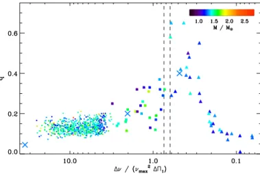
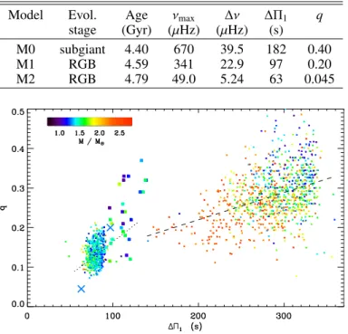
Fig. 6. Coupling factor q as a function of the mixed-mode density N = ∆ν/(∆Π1 ν2
max). The vertical dashed lines indicate the transition
from subgiants to red giants defined byMosser et al.(2014). Triangles indicate subgiants; squares indicate stars on the RGB (small squares for long-cadence Kepler data and big squares for short-cadence data). Three values of q obtained for a synthetic 1.3-M evolutionary sequence are
also shown with × (see Sect.5.3and Table3).
evolutionary stage. For interpreting observed coupling factors of clump stars, a theoretical study of strong coupling must be con-sidered (Takata 2016).
When the threshold level of the detection is increased, the spread in q decreases for clump stars. We observed that low Q values are often associated with unevenly spaced period spectra,
regardless of the signal-to-noise ratio of photometric time series. As a result, low or high q values are most often related to buoy-ancy glitches, as observed inMosser et al.(2015).
4.3. Subgiants
Subgiants were also considered. In that case, coupling factors were not measured with the aforementioned method, but were directly determined from the fit of the mixed-mode pattern. The validity of the asymptotic expression is questionable for mixed modes with low-radial gravity orders observed in red giants. It however provides period spacings that fully agree with modeled values (Benomar et al. 2013, 2014; Deheuvels et al. 2014). In fact, even if the density of gravity modes expressed by the num-ber N = ∆ν/(ν2max∆Π1) is small, the distribution of the period spacings is well reproduced by the asymptotic expression and is sensitive to q. From the quality of the fit of the mixed mode, we could measure this parameter and estimate relative uncertainties that are smaller than 20%. The identification of high q values is especially clear: in such cases, the period spacings hardly de-pend on the nature of the mixed mode (Fig.3). In Fig. 6, q is plotted as a function of the mixed-mode density N instead of∆ν to emphasize the change of physics when a subgiant evolves into a red giant. The strongest values of q, close to unity, are obtained at the transition from subgiants to red giants.
4.4. Outliers
A limited number of stars have coupling factors significantly dif-ferent from the mean behavior. We stress that their identification
B. Mosser et al.: Coupling factors of mixed mode
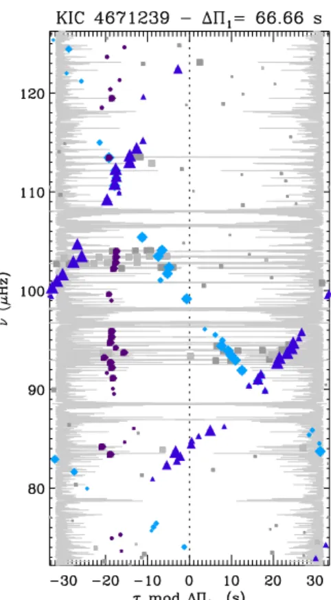
Fig. 7. Échelle diagram of the very low metallicity RGB star KIC 4671239, with the stretched period τ modulo∆Π1 on the x-axis and
frequency on the y-axis. All dark symbols indicate dipole modes with a height above 5 times the local stellar background; their sizes depend on the mode height. When the azimuthal order can be automatically iden-tified, triangles correspond to m = −1, squares to m = 0, diamonds to m= +1. Light gray symbols correspond to unidentified modes: most of these are located in the region of pressure-dominated mixed modes; a few unidentified modes may also be ` = 3 modes. All components of the rotational multiplets intersect at 112 µHz; the m= ±1 components intersect at 91 µHz. The oscillation spectrum is plotted in gray top to bottom in the background of the figure to link the stretched periods and the mixed-mode frequency.
in this work dedicated to ensemble asteroseismology is certainly incomplete; outliers are however rare. The stars we identified deserve future attention.
4.4.1. KIC 4671239
KIC 4671239 has been identified byThygesen et al.(2012) as one of the less metallic red giants observed by Kepler, with [Fe/H] = −2.45 and Teff = 4900 K. The seismic parameters of this star are highly atypical. Apart from the high coupling value for an RGB star at a similar evolutionary stage (q ' 0.25 instead of less than 0.15), the analysis of its mixed-mode pat-tern has revealed a period spacing∆Π1 ' 66.6 s, which is much smaller than for RGB stars with similar∆ν (Mosser et al. 2014; Vrard et al. 2016), and a much higher core rotation (Mosser et al. 2012a) with δνrot ' 830 nHz. These parameters translate in a complex mixed-mode pattern, in which the different azimuthal orders show intricate structures. Disentangling this pattern is only possible with an échelle diagram constructed with stretched periods (Fig.7), followingMosser et al.(2015) andGehan et al. (2016).
4.4.2. KIC 6975038
KIC 6975038 also shows atypical seismic parameters, with ∆Π1' 57.9 s, which is much smaller than comparable stars with ∆ν = 10.61 µHz, and q ' 0.35, which is much above the val-ues observed on the RGB. The low value of∆Π1and the high value of q may both indicate a larger radiative cavity, hence a smaller region where modes are evanescent, than in other stars with similar∆ν.
4.4.3. Massive stars
Stars in the secondary clump, more massive than 1.8 M , show lower q compared to less massive stars burning their core he-lium. The difficulty of fitting their mixed-mode spectrum does not resemble the difficulty met in presence of buoyancy glitches (Mosser et al. 2015). A better fit of the data can be obtained with a gradient in q as a function of frequency. According to the study conducted in Sect.2, this gradient may result from the fact that the NBVand S1profiles are not parallel in the evanescent region of such stars.
This effect appears for stars as KIC 4372082 or 6878041, which are more massive than the secondary-clump stars stud-ied by Deheuvels et al.(2015). Such objects are rare and, de-spite low-quality spectra, certainly deserve detailed study and modeling.
5. Discussion
The variation of the coupling factor with the large separation ∆ν can be used to derive direct information concerning the ex-tent of the evanescent region between the NBVand S1 profiles, with the formalism introduced in Sect.2. Even if mixed modes probe these functions in a limited frequency range around νmax, the hypothesis that the NBVand S1 profiles are parallel in the considered region helps us to derive precise information on stel-lar interior properties; regardless of the consequence of the de-crease of νmaxwith evolution. The hypothesis is finally discussed in Sect.5.4.
5.1. Variation with the evolutionary stage 5.1.1. Subgiant – red giant transition
Mosser et al.(2014) have shown that the transition between sub-giants and redsub-giants has a clear signature in the∆Π1 –∆ν dia-gram. In the subgiant phase, the relation between these asymp-totic period and frequency spacings shows a large spread with a significant mass dependence, whereas the parameters are tightly bound on the RGB. The coupling factor q is similarly impacted by the evolution and shows a significant increase at the end of the subgiant phase (Fig.6). This increase occurs in parallel with the first dredge-up, when the base of the convection zone goes deeper in the envelope. A high value of q indicates that not only the NBV profile, but also the S1 profile, is deep in the stellar interior. Observing high values in the range [0.40–0.65] near the transition region from subgiants to red giants argues, using Fig.2, for a slope β slightly higher than or close to 1.3 with a ratio α2larger than about 0.5.
5.1.2. On the RGB
At the beginning of the ascent on the RGB, the stellar core con-tracts and the envelope expands. The decrease of q means either A1, page 7 of10
Table 1. Mass dependence of q on the RGB.
M/M 1.0 1.2 1.4 1.6 1.8 2.0
qM 0.144 0.128 0.126 0.123 0.134 0.134
σq 0.021 0.025 0.026 0.022 0.023 0.027
Notes. The variation of q with∆ν is modeled as q = qM(∆ν/10)0.096,
with∆ν in µHz.
Table 2. Mass dependence of q in the red clump.
M/M 0.9 1.1 1.3 1.5 1.7 2.0
qb 0.301 0.287 0.274 0.272
¯q 0.363 0.324 0.299 0.289 0.283 0.270
qe 0.339 0.313 0.303 0.290
σq 0.024 0.016 0.011 0.010 0.012 0.022
Notes. The values qb, ¯q, and qemeasure, respectively, the coupling for
the early, middle, and late stages in the clump, defined inMosser et al.
(2014); these values are defined by 25% of the stars lying on the first, middle, and late portion of the mass-dependent evolutionary track, re-spectively; σq measures the spread of the values; the fits were derived
from high-quality spectra with Q ≥ 50.
that the region between NBVand S1expands too, inducing a de-crease of α, or that the coefficient β increases toward the value 3/2. A simultaneous variation of both terms α and β is possible too.
For evolved models on the RGB, νmaxbecomes smaller than the value of NBVat the base of the convective zone, so that the hypothesis of parallel variations of NBVand S1is no longer valid for evolved stars on the RGB (e.g., Montalbán et al. 2013). In fact, the decrease of q with stellar evolution can result either from the decrease of νmax or from the expansion of the region between NBVand S1, so that it is impossible to derive any firm conclusion in terms of interior structure evolution.
The decrease of q on the RGB plays a non-negligible role in the difficulty to observe mixed modes at small ∆ν predicted for high- and low-mass stars (Dupret et al. 2009;Grosjean et al. 2014). In fact, mixed modes that are not in the close vicinity of the pressure-dominated modes are poorly coupled, so that they show an important gravity character, hence a high inertia and tiny amplitude. In practice, measuring low values of q is hard.
In order to estimate the mass dependence of q observed on the RGB, we first fitted the slope of q(∆ν) as a power law under the assumption that the exponent does not depend on the stellar mass. In a second step, we quantified the mass dependence in the relation q(∆ν). For low-mass stars with a degenerate helium core, the higher M, the lower q; for stars more massive than 1.8 M , the situation is inverted (Table1). This change occurs near the limit in mass between the red and secondary clumps, so is likely related to the degeneracy of helium in the core.
5.1.3. In the red clump
In the red clump, the mass dependance of q is coupled to the large separation dependence: the lower the mass, the higher the coupling. This behavior is discussed in the next paragraph, since it obeys to a general trend in the relationship between q and∆Π1. Mean values of the coupling for red clump stars are given in Table 2. Using the seismic evolutionary tracks depicted in Mosser et al. (2014), we could measure the evolution of q in the red clump, at fixed mass. Values at the early, middle, and
Table 3. Seismic properties of 1.3 M models.
Model Evol. Age νmax ∆ν ∆Π1 q
stage (Gyr) (µHz) (µHz) (s)
M0 subgiant 4.40 670 39.5 182 0.40
M1 RGB 4.59 341 22.9 97 0.20
M2 RGB 4.79 49.0 5.24 63 0.045
Fig. 8. Coupling factor q as a function of the period spacing ∆Π1
for RGB and clump stars. Same symbols as in Fig.6. A threshold at Q = 100 reduces the number of stars compared to Fig.5. The dot-ted and dashed lines correspond to the fits for RGB and clump stars, respectively.
late stages in the clump are shown in Table 2. As shown by Mosser et al.(2015), the evolution of stars in the red clump show non-monotonous variation of both∆ν and ∆Π1. Conversely, the monotonous increase of q indicates either that the ratio α in-creases along the evolution of low-mass stars in the red clump, resulting from a small shrinking of the evanescent region, or that the exponent β decreases. Both effects may simultaneously con-tribute to the variations.
5.2. Variation with the period spacing
The variations of q with the period spacing∆Π1depend on the evolutionary stage. Wether on the RGB or in the clump, the global variations of q(∆Π1) indicate that the larger ∆Π1, the larger q (Fig.8). A large value of∆Π1is representative of a small dense core with high NBVvalues. So, we come to the conclusion that high values of NBVand S1 occur in similar situations, and that they get close to each other when they increase together. At fixed β, the ratio α = NBV/S1 is then correlated with ∆Π1 for both RGB and clump stars (but not for subgiants).
Since the variations of q are nearly linear in both domains, the following simple fits can be used as proxies for q (Fig.8):
qRGB = −0.0034 +∆Π 1 597, (17) qclump = 0.082 + ∆Π 1 1450, (18)
where∆Π1is measured in seconds. The fit of qRGBis however not efficient for early RGB stars; the fit of qclumpis valid for both primary and secondary clumps. Such fits are intended to facili-tate the identification of the mixed-mode pattern, rather than for explaining the physics of the coupling.
B. Mosser et al.: Coupling factors of mixed mode 5.3. Modeling and computation of q
We used stellar models to match the observed coupling fac-tor. We considered 1.3-M models at three evolutionary stages (Table 3) without overshoot or diffusion; their full description is given in Belkacem et al.(2015). In the strong coupling case (model M0), we computed q from Eqs. (12)–(14) using the asymptotic formalism of Takata (2016) and taking the pertur-bation of the gravitational potential into account. In the inter-mediate case (model M1), using a similar analysis is question-able since hypotheses in the calculation of XRare valid when the evanescent region is very thin. Nevertheless, the strong-coupling analysis matches the weak-coupling case when the evanescent region becomes very large, so that we computed q in a simi-lar way as for the model M0. In the weak coupling case (model M2), we used the same expression, but with XR = 0 and, fi-nally, compare these three factors with observations. The factor qshows in fact small variations with frequency, so that we had to consider the mean value, defined in a 4-∆ν broad frequency range centered on νmax. We checked that the term XRintroduced by Eq. (14) significantly reduces the value of q and also con-tributes to the relative stability of q with frequency. We also no-ticed that the perturbation of the gravitational potential plays a non-negligible role not only in the core but also in the evanes-cent zone and in the inner region of the convective envelope. This provides evidence that the Cowling approximation is not appropriate for computing q.
Modeling quantitatively agrees with observations, except for the most evolved model. The subgiant model M0 close to the transition to red giants shows a high q; the next model M1 is on the RGB and has a much lower q. Both agree with the ob-served values. The coupling factor for model M2, higher on the RGB, shows however a value that is significantly smaller than observed. In M2, the evanescent region is in fact above the base of the convective envelope (e.g., Fig. 2 ofMontalbán et al. 2013). This point deserves further work, which is beyond the scope of this paper.
Modeling red clump stars requires special attention in the prescription of convection and mixing in the core (Lagarde et al. 2012; Bossini et al. 2015). We could not compare our results with modeling but used the calculations exposed in Sect.2. The high values observed for q in the clump imposes the exponent β (Eq. (5)) to be less than 3/2 (Fig.2).
5.4. Variation of q with frequency
For a limited number of stars examined byVrard et al.(2016), the asymptotic expansion does not provide a satisfying fit of the mixed-mode pattern without a direct explanation in terms of buoyancy glitch. For these stars, a better fit is obtained when varying q with frequency. Modeling derives similar conclusion, with different slopes βN and βS (Eq. (5)) or more complicate variations (e.g.,Montalbán et al. 2013).
Since the independence of q with frequency derives from the hypothesis of parallel variations of NBVand S1, we have to con-clude that this hypothesis is not fully correct. The observational study of the variations of q with frequency appears to be highly challenging for the same reasons as those explaining the di fficul-ties in measuring q (rotation, glitches, and finite mode lifetimes). The individual study of bright stars with a high signal-to-noise ratio is necessary to investigate the frequency dependence of q in detail. Combined with modeling, this study will help assess to which extent the mean value of q is a global seismic parameter,
which is as informative for the evanescent region as∆ν and ∆Π1 for the pressure and radiative cavities, respectively.
6. Conclusions
The new method setup for measuring the coupling factor of mixed modes in evolved stars has provided the first analysis of this parameter over a large set of stars. We could determine 5200 values of q, from subgiants to clump stars. Three main results can be inferred:
– Coupling factors test the region between the Brunt-Väisälä cavity and the S1profile, dominated by the radiative core and the hydrogen-burning shell. Indeed, while∆ν is mainly sen-sitive to the envelope and∆Π1provides the signature for the core, we can directly access the intermediate region with q. – The variation of q with stellar evolution provides us with new
constraints on stellar modeling. We note that, for both RGB and clump stars, the coupling factors show simple global variations with the period spacing. The characterization of outliers can be used to constrain physical processes inside stars.
– Strong coupling is observed in stars at the transition subgiant/red giant and in the red clump. In fact, the weak-coupling formalism of Unno et al. (1989) fails for a quantitative use of the observed coupling factors, except for the most evolved stars on the RGB. In all other cases, the use of the new formalism proposed by Takata (2016) for strong coupling is mandatory.
These measurements also open the way to more precise fits of the mixed-mode pattern to analyze in detail extra features, such as the rotational splittings and buoyancy glitches.
Acknowledgements. We acknowledge the entire Kepler team, whose efforts made these results possible. B.M., C.P., and K.B. acknowledge financial support from the Programme National de Physique Stellaire (CNRS/INSU), from the French space agency CNES, and from the ANR program IDEE Interaction Des Étoiles et des Exoplanètes. M.T. is partially supported by JSPS KAKENHI Grant Number 26400219. M.V. acknowledges funding by Fundação para a Ciência e a Tecnologia (FCT) through the grant CIAAUP-03/2016-BPD, in the context of the project UID/FIS/04434/2013, co-funded by FEDER through the program COMPETE2020 (POCI-01-0145-FEDER-007672).
References
Bedding, T. R., Mosser, B., Huber, D., et al. 2011,Nature, 471, 608
Belkacem, K., Marques, J. P., Goupil, M. J., et al. 2015,A&A, 579, A31
Benomar, O., Bedding, T. R., Mosser, B., et al. 2013,ApJ, 767, 158
Benomar, O., Belkacem, K., Bedding, T. R., et al. 2014,ApJ, 781, L29
Bossini, D., Miglio, A., Salaris, M., et al. 2015,MNRAS, 453, 2290
Buysschaert, B., Beck, P. G., Corsaro, E., et al. 2016,A&A, 588, A82
Chaplin, W. J., Kjeldsen, H., Christensen-Dalsgaard, J., et al. 2011,Science, 332, 213
Corsaro, E., Stello, D., Huber, D., et al. 2012,ApJ, 757, 190
Cunha, M. S., Stello, D., Avelino, P. P., Christensen-Dalsgaard, J., & Townsend, R. H. D. 2015,ApJ, 805, 127
Deheuvels, S., Do˘gan, G., Goupil, M. J., et al. 2014,A&A, 564, A27
Deheuvels, S., Ballot, J., Beck, P. G., et al. 2015,A&A, 580, A96
De Ridder, J., Barban, C., Baudin, F., et al. 2009,Nature, 459, 398
Dupret, M., Belkacem, K., Samadi, R., et al. 2009,A&A, 506, 57
Epstein, C. R., Elsworth, Y. P., Johnson, J. A., et al. 2014,ApJ, 785, L28
Gaulme, P., McKeever, J., Jackiewicz, J., et al. 2016,ApJ, 832, 121
Gehan, C., Mosser, B., & Michel, E. 2016, Astro Fluid 2016 Conf. Proc., submitted [arXiv:1611.00540]
Goupil, M. J., Mosser, B., Marques, J. P., et al. 2013,A&A, 549, A75
Grosjean, M., Dupret, M.-A., Belkacem, K., et al. 2014,A&A, 572, A11
Huber, D., Bedding, T. R., Stello, D., et al. 2011,ApJ, 743, 143
Kallinger, T., Mosser, B., Hekker, S., et al. 2010,A&A, 522, A1
Kallinger, T., De Ridder, J., Hekker, S., et al. 2014,A&A, 570, A41
Lagarde, N., Decressin, T., Charbonnel, C., et al. 2012,A&A, 543, A108
Lagarde, N., Miglio, A., Eggenberger, P., et al. 2015,A&A, 580, A141
Miglio, A., Brogaard, K., Stello, D., et al. 2012,MNRAS, 419, 2077
Montalbán, J., Miglio, A., Noels, A., et al. 2012,Astrophys. Space Sci. Proc., 26, 23
Montalbán, J., Miglio, A., Noels, A., et al. 2013,ApJ, 766, 118
Mosser, B., Belkacem, K., Goupil, M., et al. 2010,A&A, 517, A22
Mosser, B., Barban, C., Montalbán, J., et al. 2011a,A&A, 532, A86
Mosser, B., Belkacem, K., Goupil, M., et al. 2011b,A&A, 525, L9
Mosser, B., Goupil, M. J., Belkacem, K., et al. 2012a,A&A, 548, A10
Mosser, B., Goupil, M. J., Belkacem, K., et al. 2012b,A&A, 540, A143
Mosser, B., Dziembowski, W. A., Belkacem, K., et al. 2013a,A&A, 559, A137
Mosser, B., Michel, E., Belkacem, K., et al. 2013b,A&A, 550, A126
Mosser, B., Benomar, O., Belkacem, K., et al. 2014,A&A, 572, L5
Mosser, B., Vrard, M., Belkacem, K., Deheuvels, S., & Goupil, M. J. 2015,
A&A, 584, A50
Mosser, B., Belkacem, K., Pincon, C., et al. 2017,A&A, 598, A62
Shibahashi, H. 1979,PASJ, 31, 87
Silva Aguirre, V., Chaplin, W. J., Ballot, J., et al. 2011,ApJ, 740, L2
Takata, M. 2016,PASJ, 68, 109
Thygesen, A. O., Frandsen, S., Bruntt, H., et al. 2012,A&A, 543, A160
Unno, W., Osaki, Y., Ando, H., Saio, H., & Shibahashi, H. 1989, Nonradial os-cillations of stars, eds. W. Unno, Y. Osaki, H. Ando, H. Saio, & H. Shibahashi Vrard, M., Mosser, B., Barban, C., et al. 2015,A&A, 579, A84