HAL Id: insu-01627902
https://hal-insu.archives-ouvertes.fr/insu-01627902
Submitted on 23 Mar 2018
HAL is a multi-disciplinary open access
archive for the deposit and dissemination of
sci-entific research documents, whether they are
pub-lished or not. The documents may come from
teaching and research institutions in France or
abroad, or from public or private research centers.
L’archive ouverte pluridisciplinaire HAL, est
destinée au dépôt et à la diffusion de documents
scientifiques de niveau recherche, publiés ou non,
émanant des établissements d’enseignement et de
recherche français ou étrangers, des laboratoires
publics ou privés.
content probability using satellite imager data
Christopher R. Yost, Kristopher M. Bedka, Patrick Minnis, Louis Nguyen,
John Walter Strapp, Rabindra Palikonda, Konstantin Khlopenkov, Douglas
Spangenberg, William L. Smith Jr., Alain Protat, et al.
To cite this version:
Christopher R. Yost, Kristopher M. Bedka, Patrick Minnis, Louis Nguyen, John Walter Strapp, et
al.. A prototype method for diagnosing high ice water content probability using satellite imager data
. Atmospheric Measurement Techniques, European Geosciences Union, 2018, 11 (3), pp.1615-1637.
�10.5194/amt-11-1615-2018�. �insu-01627902�
https://doi.org/10.5194/amt-11-1615-2018 © Author(s) 2018. This work is distributed under the Creative Commons Attribution 4.0 License.
A prototype method for diagnosing high ice water content
probability using satellite imager data
Christopher R. Yost1, Kristopher M. Bedka2, Patrick Minnis1, Louis Nguyen2, J. Walter Strapp3,
Rabindra Palikonda1, Konstantin Khlopenkov1, Douglas Spangenberg1, William L. Smith Jr.2, Alain Protat4, and Julien Delanoe5
1Science Systems and Applications, Inc., Hampton, VA 23666, USA 2NASA Langley Research Center, Hampton, VA 23681, USA 3Met Analytics Inc., Aurora, Ontario, Canada
4Australian Bureau of Meteorology, Melbourne, Australia
5Laboratoire Atmosphere, Milieux, et Observations Spatiales, Guyancourt, France
Correspondence: Kristopher M. Bedka (kristopher.m.bedka@nasa.gov) Received: 6 October 2017 – Discussion started: 1 November 2017
Revised: 6 February 2018 – Accepted: 13 February 2018 – Published: 22 March 2018
Abstract. Recent studies have found that ingestion of high mass concentrations of ice particles in regions of deep con-vective storms, with radar reflectivity considered safe for air-craft penetration, can adversely impact airair-craft engine per-formance. Previous aviation industry studies have used the term high ice water content (HIWC) to define such con-ditions. Three airborne field campaigns were conducted in 2014 and 2015 to better understand how HIWC is distributed in deep convection, both as a function of altitude and prox-imity to convective updraft regions, and to facilitate devel-opment of new methods for detecting HIWC conditions, in addition to many other research and regulatory goals. This paper describes a prototype method for detecting HIWC con-ditions using geostationary (GEO) satellite imager data cou-pled with in situ total water content (TWC) observations col-lected during the flight campaigns. Three satellite-derived parameters were determined to be most useful for determin-ing HIWC probability: (1) the horizontal proximity of the aircraft to the nearest overshooting convective updraft or tex-tured anvil cloud, (2) tropopause-relative infrared brightness temperature, and (3) daytime-only cloud optical depth. Sta-tistical fits between collocated TWC and GEO satellite pa-rameters were used to determine the membership functions for the fuzzy logic derivation of HIWC probability. The prod-ucts were demonstrated using data from several campaign flights and validated using a subset of the satellite–aircraft collocation database. The daytime HIWC probability was
found to agree quite well with TWC time trends and iden-tified extreme TWC events with high probability. Discrim-ination of HIWC was more challenging at night with IR-only information. The products show the greatest capability for discriminating TWC ≥ 0.5 g m−3. Product validation re-mains challenging due to vertical TWC uncertainties and the typically coarse spatio-temporal resolution of the GEO data.
1 Introduction
Recent studies have documented many events since the early 1990s where aircraft flight through deep convective storms and cirrus anvil outflow has resulted in jet engine power loss, loss of engine control, and/or engine damage events (Lawson et al., 1998; Mason et al., 2006; Bravin et al., 2015). Mason et al. (2006) reported that engine events occurred in seem-ingly innocuous cloud regions with only light to moderate turbulence, infrequent lightning, and where the pilot’s radar indicated green or weaker echoes (< approximately 30 dBZ). This lead to their hypothesis that the aircraft were encoun-tering high mass concentrations of small ice particles associ-ated with convective updrafts, and ice accretion in the engine by ingested ice particles was likely the cause of the events. These encounters of high mass concentrations in low radar reflectivity have been termed high ice water content (HIWC) events.
Subsequent meteorological analyses support that HIWC can be found within or near convective updrafts with a high concentration of small ice particles that would not produce a strong radar reflectivity (Platt et al., 2011; Gayet et al., 2012). Confirmation of many of the original hypotheses of Mason et al. (2006) was obtained in an exploratory in situ flight campaign in HIWC conditions (Grandin et al., 2014). In more recent years, icing of aircraft air data probes (e.g., pitot airspeed indicators) has also been recognized to occur in the same type of cloud conditions (Duvivier, 2010). The microphysical characteristics of HIWC events make this haz-ard difficult to identify and avoid based on currently available cloud information in the cockpit from weather radar.
There is currently no formal definition of HIWC, and lev-els and exposure distances required for ice accretion in en-gines have not yet been established. Individual industry re-searchers have typically chosen between 1 and 2 g m−3 as their HIWC thresholds, while accepting that 0.5 g m−3does not appear to represent a threat. Here we choose a HIWC threshold of 1 g m−3, in the belief that, pending more in-formation from ice accretion researchers on the threat lev-els, a more conservative definition is prudent for a detection scheme.
Geostationary (GEO) satellite observations and derived products have been used to analyze past HIWC events and could potentially be used to develop HIWC detection prod-ucts, assuming that HIWC events occur in a consistent set of conditions. Through analysis of GEO data from historical in-service engine icing events over Japan and Southeast Asia ex-perienced by Boeing aircraft, Bravin et al. (2015) found that these events occurred predominantly in mesoscale convective systems with relatively large anvils. The aircraft typically tra-versed through a long section (196 km on average) of cloud at or near the convective equilibrium level, also known as the level of neutral buoyancy, but also quite close (41 km on av-erage) to the center of a local area with cloud tops at least 10 K colder than the equilibrium level. These anomalously cold clouds often occur within or near “overshooting cloud tops” (OTs) which indicate small updraft cores (< 20 km di-ameter) of sufficient strength to penetrate through the anvil, typically located near to the equilibrium level. A 10 K tem-perature differential equates to more than a 2 km penetration of cloud top above anvil based on analysis of GEO imagery coincident with NASA CloudSat OT overpasses (Griffin et al., 2016). Bravin et al. (2015) showed that not only were the events close in location to such an OT, but also typically within an hour of the time of its maximum intensity, and not necessarily correlated to the time of the overall storm peak intensity.
One HIWC nowcasting approach has recently been pub-lished which seeks to maximize the HIWC event detection rate by identifying any ice cloud with moderate to high cloud optical depth (COD > 20, de Laat et al., 2017). Their ap-proach seeks to combine satellite-derived cloud parameters to identify regions where total water content (TWC) could
exceed 1 g m−3 anywhere throughout the vertical depth of a cloud. Their binary yes/no HIWC mask indicates where HIWC is possible, but does not provide information on where HIWC is likely, especially in deep convection where COD routinely exceeds 20 (Hong et al., 2007). Such an approach could identify a variety of cloud conditions where HIWC may be present, not necessarily restricted to the types of deep convection documented in Bravin et al. (2015).
The European High Altitude Ice Crystal (HAIC) and North American High Ice Water Content (HIWC) projects (Dezit-ter et al., 2013; Strapp et al., 2016a) have conducted sev-eral flight campaigns in recent years to collect in situ and remote sensing observations of ice water content within deep convective clouds at various temperature levels ranging from −10 to −50◦C, a temperature range encompassing the typ-ical ambient icing environment for aircraft climb, descent, and cruise. The overarching goal of these campaigns is to bet-ter characbet-terize the atmospheric environment that causes en-gine and air data probe failures that threaten aviation safety. The campaigns seek to (1) help assess a new aircraft mixed-phase/glaciated icing certification envelope (Mazzawy and Strapp, 2007) contained in FAA Title 14 Code of Federal Regulations Part 33 Appendix D that recently became law, by collecting in situ characterization measurements for com-parison; (2) develop techniques for the aviation industry to detect and nowcast HIWC conditions for exit and avoidance; (3) provide data for specialized aviation applications such as engine modeling, ground cloud simulation facilities, and the development of certification means of compliance; and (4) take advantage of the unique data sets the campaigns will provide to support scientific research in the characterization of deep convection, fundamental cloud microphysics, cloud modeling, and the development of radar and satellite cloud remote sensing products.
The primary goals of the HAIC and HIWC campaigns were to provide statistics on the 99th percentile of in situ total water content (TWC), and characterize other relevant cloud parameters such as ice particle size for regulatory pur-poses. The high-frequency in situ TWC observations col-lected within the HAIC and HIWC campaigns are invaluable for development of satellite-based HIWC diagnostic prod-ucts. Prior to these campaigns, a large sample of consis-tent in situ TWC data across diverse geographic regions had been lacking, which had prohibited HIWC diagnostic prod-uct development. GEO satellite imagers such as the Mul-tifunction Transport Satellite (MTSAT) Japanese Meteoro-logical Imager (JAMI), Geostationary Operational Environ-mental Satellite (GOES), and Meteosat Second Generation Spinning Enhanced Visible and Infrared Imager (SEVIRI) observed deep convective clouds throughout their lifecycles in 5 to 30 min intervals during the HAIC and HIWC cam-paigns, depending on the geographic region. GOES-14 ob-servations were also collected at up to 1 min intervals on two flight days during a Super Rapid Scan Operations for GOES-R (SGOES-RSOGOES-R, Schmit et al., 2014) period. GEO imager
ob-servations and associated derived products depict storm in-tensity, locations of intense updrafts, and cloud-top micro-physical characteristics that have previously been analyzed for a small sample of HIWC events. A more comprehensive analysis of GEO imagery relative to aircraft TWC measure-ments enables the research community to better understand the characteristics and evolution of clouds that do and do not produce HIWC. This understanding is critical for the devel-opment of satellite-based HIWC detection products.
This paper has two primary objectives, (1) to provide sta-tistical analyses of cloud properties derived from GEO ob-servations as a function of TWC using data from three re-cent flight campaigns and (2) to develop and demonstrate a prototype satellite-based probability of HIWC (PHIWC) di-agnostic product. The three campaigns analyzed in this pa-per were the two HAIC-HIWC campaigns centered in Dar-win, Australia in January–March 2014 and Cayenne, French Guiana in May 2015, and the NASA HIWC-RADAR cam-paign centered in Fort Lauderdale, Florida, in August 2015. The prototype algorithm developed here provides a more pre-cise method for near-real time avoidance of HIWC condi-tions than previously available.
2 Datasets
2.1 Experiment and flight campaign descriptions In 2006, an industry working group tasked by the FAA to re-view issues related to mixed-phase and glaciated icing condi-tions recommended the collection of a new in situ data set to characterize the microphysical properties of deep convective clouds, the type that had been identified as causing engine events. The HIWC Study was then initiated within North America and initially worked on the modification and de-velopment of new instrumentation required to make accurate measurements in hostile convective conditions, while plans for a flight campaign were developed.
In 2012, the HIWC team partnered with the HAIC Project to conduct the first HAIC-HIWC flight campaign (hereafter Darwin-2014) in Darwin, Australia using the SAFIRE Fal-con 20 aircraft. The flight program was successfully Fal- con-ducted between 16 January and 18 February 2014, but fell short of its data collection goal due to an engine failure unrelated to engine icing. A total of 23 flights were con-ducted, mostly in large tropical mesoscale convective sys-tems (MCSs). In addition to a new IKP2 TWC measurement device (described in the next section), the Falcon 20 cloud measurement instrument suite included a Droplet Measure-ment Technologies (DMT) Cloud Droplet Probe (CDP-2; 2– 49 µm), a Stratton Park Engineering Co. 2D-S imaging probe (10–1280 µm), and a DMT Precipitation Imaging Probe (PIP; 100–6400 µm). A Science Engineering Associates Robust hot-wire probe (Strapp et al., 2008; Grandin et al., 2014) pro-vided backup TWC measurements. The RASTA (RAdar
Sys-Tem Airborne) research W-band radar (Protat et al., 2004) provided Doppler and reflectivity radar measurements from six antennae.
The second HAIC-HIWC flight campaign (hereafter Cayenne-2015) was conducted from 5–29 May 2015 out of Cayenne, French Guiana. Two aircraft collected cloud in situ data from this campaign: the Falcon 20 with approximately the same instrument suite as described above, and the Na-tional Research Council of Canada Convair-580 aircraft, also equipped for cloud in situ and remote sensing. The details of the many Convair instruments will not be provided here, but it carried a second copy of the IKP2 probe for primary TWC measurements, and the CDP-2, 2D-S, and PIP for par-ticle size distribution measurements. A total of 17 Falcon 20 and 10 Convair-580 flights provided data from oceanic MCS and continental storms that were suitable for the HIWC cloud analysis.
The NASA HIWC-RADAR flight campaign (hereafter Florida-2015) was conducted from 12 to 28 August 2015, with a base of operations in Fort Lauderdale, Florida. The NASA DC-8 aircraft was equipped with the IKP2 TWC probe, CDP-2, 2D-S, and PIP as primary cloud in situ in-strumentation. A total of 10 flights were conducted off the southeast coast of the USA, the Gulf of Mexico, and over the Caribbean. Although the primary objective of this cam-paign was to test pilot radar technologies, the project adopted the same cloud measurement strategies, focusing on oceanic MCS. The measurements included four flights in tropical storms Danny and Erika.
The overall objective of the three flight campaigns was to collect data to support the aviation industry objectives, and thus the flights were designed and funded with the first priority to collect cloud characterization data in the types of clouds that cause engine events, and in regions of those clouds that would be similar to what a commercial aircraft pilot might traverse. These objectives were not necessarily compatible with collection of the best scientific data. The flight plans, described in the HIWC Science and Technical Plan (Strapp et al., 2016a), were adopted for all three cam-paigns. The plans call for quasi straight-and-level runs across convectively active regions of tropical oceanic MCS clouds, similar to those described by Grzych and Mason (2010). These runs were to be aligned with regions of expected heavy rain below the aircraft, but through at most low reflectivity “green” echoes on the pilot’s radar. The pilot was given the discretion to optimize the run using his radar, and set up a pattern of reciprocal runs to survey this suspected area of HIWC. If regions of high radar reflectivity were observed at flight altitude, the pilot was instructed to traverse the sys-tem at a conventional safe proximity from the reflectivity core. Regions of lightning were to be avoided. The objec-tive was to collect at least one hundred 32.2 km data seg-ments (a regulatory reference distance) at each of the four primary temperature layers −50, −40, −30, and −10◦C, ±5◦C (in order of priority). The combination of the three
projects achieved the data collection objectives, with a total of more than 54 800 km of in-cloud data in mostly tropical oceanic MCS.
2.2 In situ total water content measurements
The measurements of these flight campaigns were expected to be dominated by ice particles in concentrations that could, at least in theory, reach 8–9 g m−3in the unlikely event that deep adiabatic cores were encountered. Although various methods have been used to make airborne TWC estimates, including evaporators, these measurements have been espe-cially problematic in a high-altitude, high-speed, HIWC en-vironment, and lack substantive information on absolute ac-curacy. The aviation group tasked to develop the technology plan that recommended the flight measurement campaigns examined reliability and accuracy information for existing airborne TWC instruments and concluded that a new instru-ment was required to reduce risk and provide more defensi-ble accuracy. It was therefore decided to develop a new TWC instrument specially designed for this environment.
The new prototype isokinetic TWC evaporator (IKP1) was designed specifically for the high-altitude, high-speed, HIWC environment, with a design goal of 20 % accuracy at 10 g m−3, 20 KPa, and 200 m s−1 true airspeed (Davison et al., 2008, 2010). The probe was downsized to a sec-ond version (IKP2) for use on the Falcon 20 aircraft, and then successfully tested in a series of wind tunnel experi-ments, exposing it to IWCs as high as 15 g m−3under high-altitude flight conditions (Strapp et al., 2016b). Accuracy es-timates to date have been provided by Davison et al. (2016) and Strapp et al. (2016b). System accuracy estimates pre-dict no more than 10 % error at all TWC values larger than about 0.1 g m−3 for temperatures colder than −30◦C. At warmer temperatures, uncertainty rises due to the increas-ing magnitude of the background humidity, which must be subtracted from the IKP2 humidity signal. This produces a baseline uncertainty, limiting the practical use of the probe to about 0◦C and colder, with the greatest effect on low TWC measurements. For the flight programs described herein, the IKP2 was the primary instrument for the TWC measurements (Strapp, 2016a, b, 2017); it has so far been concluded that it provided high TWC measurements at the desired accuracy within the target (−10 to −50◦C) temperature intervals.
The measurements of the three campaigns have revealed that ice particles dominated the TWC in the large deep con-vective clouds sampled. Mixed phase regions were narrow and infrequent, and contained only low liquid water contents. In this regard, the terms HIWC and high TWC are synony-mous for the purposes of this paper. HIWC will be used as a generic term to denote the condition, and high TWC will be used when referring to the measurement.
TWC values measured during the flight program reached a maximum of about 4.1 g m−3over a 0.93 km distance scale, the shortest scale length that is provided for this dataset.
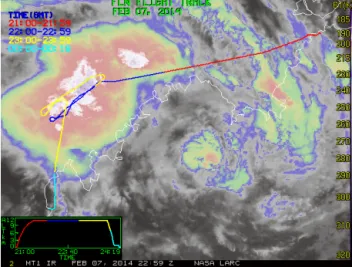
Figure 1. Flight track of the Falcon 20 on 7 February 2014, which departed from Darwin, Australia (red segment) and landed in Broome (cyan segment), overlaid upon a MTSAT-1R JAMI color-enhanced BTW image at 22:59 UTC. The track is color coded by the time of observation specified in the upper-left.
Extended periods of HIWC, defined as TWC ≥ 1.0 g m−3, were not uncommon, with 92.6 km averaged TWC values reaching as high as 2.3 g m−3. An example of a flight pat-tern conducted during Darwin-2014 Flight 16 is shown in Fig. 1. The IR image is color-enhanced such that the broad white area with embedded purple is at −78◦C or colder,
this temperature threshold being an overall informal esti-mate of the convective equilibrium level used during the project, and about 7◦C warmer than the value estimated for this day. The WMO-defined (World Meteorological Organi-zation, 1957) and cold point tropopause values were about −76 and −90◦C respectively from the nearby Broome, Aus-tralia 8 February 2014 00:00 UTC radiosonde. In this case, the distance the aircraft traversed through clouds defined by the white area of the image are unusually long for this project at about 140 nmi. The peak TWC observed during this flight was approximately 2.5 g m−3, and there were particularly long periods of sustained TWC greater than 1.5 g m−3(see Fig. 8c).
2.3 Satellite observations and derived products
During the field campaigns, satellite data were ingested and analyzed in near-real time to provide mission planning sup-port and post-mission studies. The data were utilized on site and distributed to various science team groups via the inter-net, where they remain available in digital and image formats (http://satcorps.larc.nasa.gov).
2.3.1 Satellite imager observations
Multispectral GEO satellite observations from the MTSAT-1R JAMI, and GOES-13 and GOES-14 Imagers are used
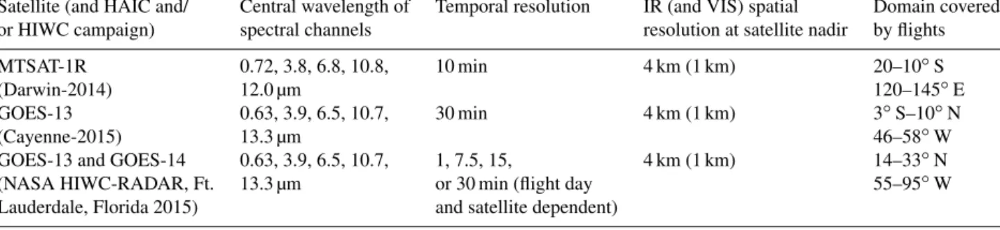
Table 1. The spectral channels, temporal and spatial resolution, of the two satellite imagers used in this study and the geographic bounds of the study domains.
Satellite (and HAIC and/ Central wavelength of Temporal resolution IR (and VIS) spatial Domain covered or HIWC campaign) spectral channels resolution at satellite nadir by flights MTSAT-1R 0.72, 3.8, 6.8, 10.8, 10 min 4 km (1 km) 20–10◦S
(Darwin-2014) 12.0 µm 120–145◦E
GOES-13 0.63, 3.9, 6.5, 10.7, 30 min 4 km (1 km) 3◦S–10◦N
(Cayenne-2015) 13.3 µm 46–58◦W
GOES-13 and GOES-14 0.63, 3.9, 6.5, 10.7, 1, 7.5, 15, 4 km (1 km) 14–33◦N (NASA HIWC-RADAR, Ft. 13.3 µm or 30 min (flight day 55–95◦W Lauderdale, Florida 2015) and satellite dependent)
to analyze convective cloud characteristics for a variety of observed IWC conditions and to produce the cloud prop-erty retrieval and overshooting convective cloud top (OT) detection products described below. Observations from the visible (VIS) and four infrared (IR) JAMI and GOES spec-tral channels are used to derive these products. These data were acquired from the University of Wisconsin Space Sci-ence and Engineering Center using the Man-computer Inter-active Data Access System-X (McIDAS-X, Lazzarra et al., 1999). Table 1 summarizes the spectral channels, the spa-tial and temporal resolution of the observations, and the ge-ographic boundaries of domains of interest for the HAIC-HIWC Darwin-2014, Cayenne-2015, and NASA HAIC- HIWC-RADAR Florida-2015 flight campaigns. The Meteosat Sec-ond Generation (MSG) SEVIRI also observed the Cayenne-2015 campaign domain at 15 min intervals, but its data were not used in this study for the following reasons: (1) MSG observes this domain at a very oblique angle (61◦) which can adversely impact cloud property retrieval accuracy and increase parallax errors, and (2) the MSG 1 km VIS data re-quired for daytime OT detection is unavailable for most of the daylight hours over this region.
2.3.2 Satellite-derived cloud property retrievals Cloud properties are retrieved from 4 km resolution GOES and MTSAT JAMI imager radiances for pixels classified as cloudy using the Satellite ClOud and Radiation Prop-erty retrieval System (SatCORPS) that identifies cloudy pix-els (Minnis et al., 2008a, b), retrieves the cloud properties (Minnis et al., 2008b, 2011), and estimates radiative fluxes from multispectral satellite imagery. For daytime portions of the images, defined as solar zenith angle (SZA) ≤ 82◦,
the Visible Infrared Shortwave-Infrared Split-Window Tech-nique (VISST) is used to retrieve cloud properties such as thermodynamic phase, cloud optical depth (COD), ice par-ticle or water droplet effective radius (Reff), cloud height,
pressure, temperature, and geometric thickness. The Solar Infrared Split-Window Technique (SIST) is used to retrieve these parameters at night. It is important to note that the SIST IR-only COD is limited to values of approximately six
and therefore is insensitive to optical depth variations within optically thick deep convective cloud tops, so only daytime VISST COD is employed in our study. The 1 km VIS data provided by GOES and MTSAT were subsetted to 4 km to match the resolution of the IR channels. The cloud phase al-gorithm classifies a cloudy pixel as either “liquid” or “ice” based on the cloud-top temperature and Reffinformation.
Op-tically thick clouds containing both liquid and ice are gener-ally classified as ice clouds since the current version of the retrieval algorithm is unable to separately classify mixed-phase clouds. Ice water path (IWP) is not directly retrieved by VISST but is rather a parameter derived from COD and Reff that is intended to represent the total amount of water
within the depth of vertically homogeneous clouds classified as having ice tops. Cloud phase is combined with aircraft air temperature observations to ensure that both satellite and aircraft were sampling glaciated clouds. Full descriptions of VISST and SIST are provided by Minnis et al. (2011). For ice clouds, the reflectance model based on severely rough-ened hexagonal ice columns (Yang et al., 2008) replaces the smooth crystal model used in Minnis et al. (2011).
The VISST COD retrieval is designed to translate the ob-served VIS reflectance into COD through the use of cloud microphysical models and knowledge of solar illumination and sensor viewing geometry. There can be significant spatial variability in VIS reflectance within deep convective cloud tops due to shadowing induced by vertical perturbations such as gravity wave and OT signatures. This is especially true at high SZA when the sun-facing sides of the vertical pertur-bation are illuminated, enhancing VIS reflectance, while the other side is shadowed. The dark shadowed regions will yield a lower COD even though they have very similar cloud mi-crophysics at the 4 km pixel scale as the brighter regions. We show later in this paper that high TWC is more likely in high COD regions, so low COD induced by shadowing would adversely impact our daytime PHIWC diagnostic product. Therefore, we smooth the COD using a 5 × 5 pixel box, weighting the center of the box by nine, the inner three-pixel frame by three, and the outer five-pixel frame by one to pre-serve locally bright clouds but also to reduce shadowing ar-tifacts. These weights were selected based upon empirical
testing. Examples of the VIS reflectance, unsmoothed COD, and smoothed COD products are shown in Fig. 2. In the un-smoothed COD (Fig. 2e), OT regions and deep convection are identified by high COD but gravity waves and other tex-tured/shadowed regions induce lower COD and what may be considered to be “noise”. In the smoothed COD (Fig. 2f), the noise is greatly reduced but the high COD in deep con-vective anvils is preserved. The smoothing process does not remove the COD biases but it provides a more spatially co-herent product which is our intent.
2.3.3 Automated deep convection and overshooting cloud top detection methods
Deep convective anvil clouds and embedded updraft (i.e., OT) regions are detected and analyzed within GEO imagery using several automated methods. A commonly used method for deep convective anvil detection is the brightness temper-ature difference (BTD) between the ∼ 6.5 µm water vapor (WV) and ∼ 10.7 µm window (BTW) channels (Schmetz et al., 1997; Martin et al., 2008). Comparisons of the BTD prod-uct with CloudSat Cloud Profiling Radar observations indi-cate that positive BTD values are effective for detection of deep convection, often with a cloud vertical thickness ex-ceeding 12 km (Young et al., 2012). This method has not proven to be effective for differentiating overshooting cloud tops (OT) from deep convective anvils (Bedka et al., 2010; Setvak et al., 2013), but increasingly positive BTD values have been correlated with intense storms and a higher likeli-hood of lightning (Machado et al., 2009).
An automated satellite-based OT detection method has been used to identify the locations of anvil clouds and deep convective updrafts within these clouds (Bedka and Khlopenkov, 2016). OTs often appear in satellite imagery as small clusters of pixels having cold BTW and enhanced texture in the VIS channel relative to the surrounding anvil, which has much more uniform BTW and smoother texture. A set of statistical, spatial, frequency analyses were devel-oped to identify clouds that could be within convection and to detect embedded BTW minima and textured regions. A set of OT candidate regions corresponding to local BTW min-ima are initially defined. The region around OT candidates is then analyzed to define the spatial extent of the anvil cloud. The anvil cloud boundary is identified by a rapid BTW crease indicative of anvil edge or sharp BTW fluctuations in-dicative of breaks in the anvil between neighboring storms. OT candidate regions that pass an extensive set of tests that quantify how closely a candidate resembles a typical OT are assigned a final “OT Probability” based on three parameters: the temperature differences between the OT candidate mini-mum BTW and (1) the surrounding anvil mean BTW, (2) the tropopause temperature derived from the WMO lapse-rate definition, and (3) the most unstable equilibrium level tem-perature. Parameters 2 and 3 are derived from the Modern-Era Retrospective Analysis for Research and Applications
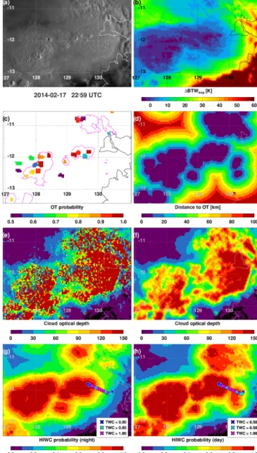
Figure 2. A series of MTSAT-1R JAMI observations and derived products for an image during Falcon 20 Flight 22 of Darwin-2014, timestamped at 22:59 UTC but valid over Australia at 23:02 UTC on 17 February 2014. (a) 0.73 µm VIS reflectance, (b) the difference between the 10.8 µm IR BT and MERRA tropopause temperature (1BTW), (c) OT Probability ≥ 0.5 (colored shading) and VIS Rat-ing ≥ 5 (magenta contours), (d) dOT, (e) original unsmoothed COD, (f) smoothed COD, (g) PHIWCnight, and (h) PHIWCday. Panels (g) and (h) are overlaid with 45 s mean TWC observations from 22:57 to 23:07 UTC.
data (MERRA, Rienecker et al., 2011), but these parameters could also be derived from any analysis or forecast for real-time applications. The OT Probability product was trained on a large sample of OT signatures and non-OT anvil cloud, with the intent to assign high probability to prominent OT signa-tures and low probability to subtle within-anvil BTW minima that are less likely to be an OT. Of the three parameters listed
above, the OT-anvil BTW difference has the greatest impact on OT Probability.
The texture in VIS imagery is quantified via a unitless “VIS Rating”. The VIS Rating product is based on pattern recognition within Fourier transform analyses of small win-dows (32 × 32 ∼ 1 km VIS pixels) of pixels with VIS re-flectance consistent with optically thick anvils observed at a particular location and time of day/year. OTs and grav-ity waves produce a unique signature within the Fourier spectrum, and the prominence of this signature is quanti-fied to derive the VIS Rating. Although VIS Rating values can exceed 50 for the most prominent OTs that penetrate the tropopause by 2+ km (Sandmael et al., 2017), values greater than seven were found within a majority of human-identified OTs (Bedka and Khlopenkov, 2016). Values as low as five identify enhanced cloud-top texture indicative of vertical mo-tions within the cloud or gravity waves and possible gener-ation of HIWC, but these low VIS Rating regions often do not correspond with the classic “cauliflower-like” signature that a human would consider to be an OT. The VIS imagery is processed at its original 1 km resolution within the OT tex-ture detection algorithm, but the maximum VIS Rating for each 4 km IR pixel region is recorded in the final VIS Rating product.
The OT detection algorithm offered a 69 % POD and 18 % FAR when high probability (≥ 0.7) BTW-based OT detections were compared against a large sample of human OT identifications within 0.25 km MODIS VIS imagery in Bedka and Khlopenkov (2016). These accuracy statistics are based on automated detections using MODIS imagery sam-pled to a 4 km resolution, representative of MTSAT JAMI and GOES imager data analyzed in this paper. The POD and FAR changed to 51 and 2 %, respectively, when high OT Probability detections were collocated with VIS Rating, il-lustrating that VIS texture detection can be used during day-time to confine the BTW-based product almost exclusively to OT regions. Areas with a non-zero VIS Rating outside of human-identified OT regions in GOES-14 imagery often co-incided with regions of > 30 dBZ radar echoes at a 10 km alti-tude for a case over the US, indicating the presence of strong updrafts (Bedka and Khlopenkov, 2016). In this paper, we will consider an “OT or texture detection” to be an OT Prob-ability ≥ 0.5 or VIS Rating ≥ 5 to attempt to capture all re-gions within or near strong vertical motions that generate de-tectable perturbations within the satellite-observed cloud top. Bedka and Khlopenkov (2016) provide a more comprehen-sive OT detection algorithm description and additional prod-uct examples.
Within an anvil cirrus cloud, BTW is well correlated with the level of neutral buoyancy temperature, which can vary regionally and seasonally (Takahashi and Luo, 2012; Bedka and Khlopenkov, 2016). Therefore, use of a fixed BTW threshold to discriminate HIWC conditions will not work across the globe so the BTW must be normalized. The com-putation of the level of neutral buoyancy is very sensitive to
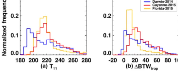
Figure 3. Distributions of BTW (a) and 1BTW (b) differentiated by HIWC and HAIC flight campaign using the colors shown in the legend.
the boundary layer temperature and moisture profile, and re-analyses such as MERRA may not capture the actual bound-ary layer structure present at the place and time of a satellite-observed storm. These inaccuracies can bias the derived level of neutral buoyancy and adversely impact BTW normaliza-tion. A more temporally and spatially stable reference for BTW is the tropopause temperature. The difference between BTW and the MERRA tropopause temperature (denoted as 1BTW hereafter) provides a globally consistent metric of storm intensity. Distributions of BTW and 1BTW along air-craft tracks during the three flight campaigns are shown in Fig. 3. We have defined 1BTW as BTW minus the MERRA tropopause temperature, so negative 1BTW corresponds to cloud tops colder than the tropopause temperature. Clouds most frequently sampled in Darwin-2014 had cloud tops ap-proximately 25 K colder than those from Cayenne-2015 or Florida-2015 due to a higher mean level of neutral buoyancy and tropopause in the Darwin region. Normalizing BTW by the tropopause temperature shows that Darwin cloud tops were only about 5–10 K colder than Florida, but still much colder (∼ 20 K) than Cayenne.
Examples of MTSAT JAMI OT detection products for a specific time during a Darwin-2014 campaign flight are shown in Fig. 2c. The corresponding VIS reflectance and 1BTW images (Fig. 2a–b) show numerous OT signa-tures present within 1BTW ≤ 5 K in the center and lower left. Highly textured cloud without evidence of a classic “cauliflower-like” OT signature is present in the upper right. Gravity waves are evident throughout the anvil cloud via rip-ples in VIS texture emanating away from OT regions. Areas within and near OTs and other textured regions are detected by the VIS Rating product (magenta contour, Fig. 2c). Es-pecially cold and distinct BTW regions collocated with VIS Rating detections are assigned high OT probability (> 0.7). Several other localized cold spots outside of textured regions in cold cirrus outflow and gravity waves are assigned lower OT Probability. Bravin et al. (2015) concluded that HIWC must often be present in outflow near to OT regions that are considered safe to traverse by pilots due to the presence of weak or non-existent echoes from onboard pilot-radar sys-tems. We developed a distance-from-the-nearest OT (dOT) product (Fig. 2d) to quantify dOT–HIWC relationships and
verify the findings of Bravin et al. (2015) using a much larger sample size. The dOT product will be discussed extensively in Sect. 3.
2.4 Satellite and aircraft collocations
Satellite observations, cloud property retrievals, and OT de-tections were collocated with the aircraft TWC observations to characterize satellite-derived cloud conditions for a range of TWC and to develop the PHIWC product. The 4 km nom-inal resolution of the satellite observations is far too coarse to resolve details at the 0.93 km scale of aircraft TWC ob-servations. The 5 s TWC observations were averaged to 45 s intervals, an approximately 8 km distance based on a nomi-nal aircraft cruising speed, in order to reduce subpixel scale variability and derive values more representative of the area within a GEO imager pixel. The maximum allowed time difference between the aircraft measurements and matching satellite observations is equal to the temporal resolution of the imagery, listed in Table 1, with Cayenne-2015 sampled at the lowest frequency on average. The four nearest satellite pixels (i.e., a 2 × 2-pixel box) were matched to the mid-point of each of the 45 s segments and the mean cloud properties were computed within this box to account for uncertainty in cloud position within the time window. Parallax corrections were based on the retrieved cloud top height and pixel loca-tion relative to GEO satellite nadir.
It is important to consider only the matches where the aircraft was physically located within cloud, and not above cloud top or below cloud base. We consider a data point to be in-cloud when TWC ≥ 0.1 g m−3. In total, 5371 satellite– aircraft matched 45 s data points within cloud were de-rived from the 50 flights during the three flight campaigns. 4598 of the matches occurred during daytime, defined by SZA ≤ 82◦. 67 % of the matches were used for PHIWC product training and the remaining 33 % were used for validation, described in Sect. 3.5. We cluster our satellite datasets into three TWC categories with low, moderate, and high TWC defined as 0.1 ≤ TWC < 0.5, 0.5 ≤ TWC < 1.0, and TWC ≥ 1.0 g m−3, respectively, for discussion purposes. TWCs of 0.5, 1.0, and 2.0 g m−3correspond to the 50th, 75th, and 95th percentiles, respectively, for this specific satellite– aircraft matched dataset. Note that the matched aircraft-satellite dataset discussed in this article is different from the dataset used for the HAIC-HIWC and NASA HIWC-RADAR regulatory analysis. The latter will supersede the dataset of this article for any regulatory purposes.
3 Results
We begin our presentation of the results by showing compar-isons of satellite observations, GEO satellite-derived prod-ucts, and in situ aircraft observations for a flight during the Darwin-2014 campaign to demonstrate the set of satellite
products most relevant for incorporation into the PHIWC di-agnostic product. We then show how select satellite products relate to aircraft TWC using the 5371 matched data pairs. We follow with a description of the PHIWC diagnostic and conclude this section with PHIWC examples and validation. 3.1 GEO satellite products and in situ TWC
comparisons
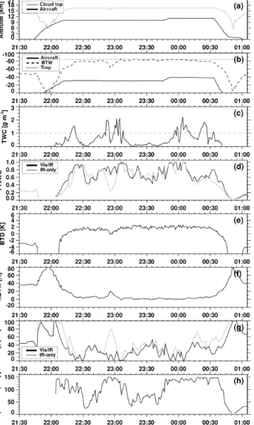
Flight 22 of the Darwin-2014 campaign, the Falcon 20 took off from Darwin around 21:45 UTC on 17 February 2014, sampled convective cells to the west over the Timor Sea, and returned to Darwin around 01:00 UTC on 18 February. A time series of observations and derived products using the satellite–aircraft matched dataset for Flight 22 is shown in Fig. 4. Cloud top heights were ∼ 16 km for the duration of the flight corresponding to BTW around −80◦C (Fig. 4a–
b). TWC measurements were collected at two distinct flight levels, the first at −30◦C from 22:10 to 23:45 UTC and the second at −40◦C from 23:50 to 00:35 UTC (Fig. 4b), which were approximately 5–6 km below our cloud top estimate. There were eight periods when TWC exceeded 1 g m−3and two periods, 22:30–22:45 and 23:15–23:50 UTC, when TWC was relatively low (< 0.25 g m−3).
TWC is not well correlated with BTW, 1BTW, or BTD during this flight, indicating that high TWC was present only in small regions within or beneath deep convective anvils (Fig. 4b–c, e–f). BTW was consistently less than −80◦C and 1BTW near 0 K but the TWC varied considerably with many periods of TWC near to or below 0.1 g m−3. From 23:15 to 00:00 UTC, BTD was greater than +1 K but varied by < 1 K as TWC increased steadily from ∼ 0.01 to > 1 g m−3. This 1 K BTD variability is extremely small and within the noise of the MTSAT-1R JAMI WV absorption channel (Ai et al., 2017), so the BTD is not useful for discriminating HIWC in this case.
High TWC was observed in many instances when the aircraft flew close to OT detections and in regions of high COD (Fig. 4g–h), showing that identification of small scale dynamical and microphysical variability in broad and very cold cloud tops is critical for discriminating HIWC condi-tions. The Falcon 20 was within 20 km of an OT detection from 22:20–22:30, 22:55–23:10, 23:50–00:05, and 00:30– 00:35 UTC and sampled high TWC in all four encounters. TWC < 0.2 g m−3 was observed during three other periods when the aircraft flew within 20 km of an OT (23:21, 23:42, and 23:47 UTC). The COD was generally above 100 for all eight HIWC periods, but there were short intervals when COD > 100 and TWC < 0.25 g m−3, illustrating the challenge associated with using passive GEO imager observations for isolating HIWC conditions at a particular flight level. Sus-tained TWC minima around 22:35 and 23:15–23:40 UTC correspond to periods with the lowest COD (25–60) during the flight. For reference, COD > 37 typically indicates deep convection (Hong et al., 2007) and values exceeding 100
in-Figure 4. Time series of matched aircraft and satellite observations for Flight 22 of Darwin-2014 on 17–18 February 2014. (a) Satel-lite retrieval of cloud top height (grey) and the altitude of the Fal-con 20 (black). (b) Satellite BTW observations (dashed), MERRA tropopause temperature analysis (dotted), and aircraft static air tem-perature observations (solid). (c) In situ 45 s averages of IKP2 TWC measurements. The dashed line indicates TWC = 1 g m−3. (d) PHIWCday(black) and PHIWCnight(grey), (e) WV-IRW BTD, (f) 1BTW (g) dOT VIS+IR (black) and IR-only (grey) and (h) smoothed COD. Major and minor tick marks represent half-hourly and 5 min intervals, respectively.
dicate extremely optically thick cloud at or near deep con-vective cores.
3.2 Analysis of cloud properties as a function of TWC The analyses from Flight 22 on 17–18 February 2014 show that the BTD and 1BTW products identify broad deep con-vective anvil cloud regions while dOT and COD resolve
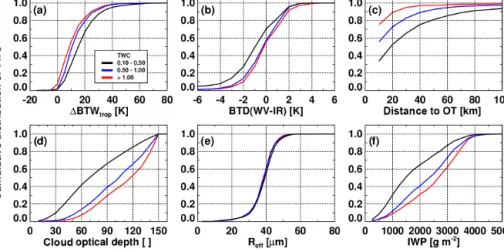
smaller-scale structures within the anvil that are better corre-lated with TWC variability. Nevertheless, these results only represent one flight and it is important to examine how these and other parameters relate to TWC observed through-out the three flight campaigns. Figure 5 shows CFDs of satellite-derived cloud properties for low, moderate, and high TWC conditions. To aid interpretation of the CFDs, we fo-cus on Fig. 5c which features the clearest separation be-tween the three TWC intervals as a function of distance to the nearest OT pixel. This panel shows that 34/56/75 % of low/moderate/high TWC events occurred within 10 km of an OT detection and 81/92/98 % occurred within 50 km of an OT.
There is a clear separation between the satellite-derived cloud properties for the low TWC and the two larger TWC intervals for all satellite parameters except Reff (Fig. 5e).
Low TWC values occur in warmer, less optically thick clouds that are farther from the nearest OT region than clouds with moderate or high TWC (Fig. 5a, d). IWP (Fig. 5f) is a param-eter based on Reffand COD, so given that Reff provides no
ability to discriminate between the TWC intervals, any sep-aration between curves in the IWP plot is entirely driven by COD. Thus, despite the fact that de Laat et al. (2017) used IWP in their HIWC mask, we feel that IWP (as currently de-fined for satellite remote sensing) appears to be a redundant covariant with COD for HIWC identification. Thus, IWP is excluded from further consideration in the algorithm formu-lation.
Differences between the moderate and high TWC cate-gories are quite small for 1BTW and BTD (Fig. 5b) but much greater for COD and dOT. High TWC occurred in flight within or beneath anvils that were slightly (3 K) colder, a bit more characteristic of deep convection (0.2 K BTD in-crease), more optically thick (∼ 15 COD units), and 6 % more likely to be within 50 km of an OT region than mod-erate TWC events. Thus, it is clear that either modmod-erate or high TWC can be present within or beneath deep convective cloud tops but high TWC occurs predominantly near updraft cores, textured gravity wave regions, and optically thick and thus ice-laden cirrus outflow.
3.3 Probability of high ice water content (PHIWC) diagnostic product description
The fundamental goal of the PHIWC diagnostic product is to optimally combine a set of satellite-derived parameters to assign high PHIWC to high TWC environments and much lower PHIWC to low and moderate TWC environments. The results from Fig. 5 show that our primary challenge will be differentiating moderate from high TWC, caused by the fact that GEO satellite imagers are most sensitive to cloud top and vertical integral parameters, leaving us to infer processes occurring within the cloud at flight level from temperature, reflectance, and spatial patterns at the cloud top. The most promising parameters to include in the PHIWC model are
Figure 5. Cumulative frequency diagrams of satellite-derived (a) 1BTW, (b) BTD, (c) dOT, (d) COD, (e) Reff, and (f) IWP for the three TWC intervals indicated in the legend in panel (a).
COD and dOT. We also include 1BTW to (1) address the fact that not every OT is accurately detected, so pixels with low 1BTW far from the nearest OT can still achieve a relatively high PHIWC; and (2) to provide additional information to the PHIWC model at night given that VIS-based predictors are unavailable. Previous studies (Bedka et al., 2010, 2012) and Fig. 5b show that BTD does not offer unique informa-tion beyond that provided by 1BTW. In addiinforma-tion, the spec-tral coverage of WV channels across the global constellation of GEO imagers differs slightly which causes differences in the observed BTs, resulting in inter-satellite inconsistencies in PHIWC product output. For these reasons, BTD will not be considered further in the algorithm formulation.
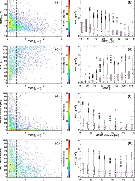
Another way to view the relationships between COD, dOT, 1BTW and TWC is in the form of scatterplots, shown in the left panels of Fig. 6. TWC increases sharply as a cloud reaches a height within 15 K of the tropopause, but then only increases slightly as the cloud top reaches or exceeds the tropopause height. There were many observations of low TWC for 1BTW near 0 K, so cold cloud temperatures alone are an insufficient discriminator of HIWC. TWC also gener-ally increases with increasing COD, but significant scatter is evident. Scatter may be due to lingering “noise” within the COD field due to shadowing/texture that we were unable to smooth as described in Sect. 2.3.2. TWC > 0.5 g m−3seldom occurs with COD < 37, the Hong et al. (2007) deep convec-tion criterion. The best HIWC discriminator appears to be the VIS+IR dOT, with a concentration of TWC > 0.5 g m−3 val-ues at dOT < 10 km. A VIS rating ≥ 5 encompasses a much larger area than an IR OT detection which helps to explain the differences between the distributions for dOT with and without VIS information. Nevertheless it is extremely rare for more extreme TWC values (≥ 2.0 g m−3)to occur out-side of a VIS+IR dOT of 20 km, highlighting the importance of including detection of textured cloud tops in the PHIWC product.
For all parameters discussed here, a TWC threshold of 0.5 g m−3 (50th percentile of TWC, vertical dashed line in Fig. 6) appears to be a breakpoint in the distributions where the satellite-based parameters begin to lose sensitivity. A use-ful PHIWC product should be able to discriminate regions with TWC ≥ 0.5 g m−3. This TWC threshold is used to de-fine a correct vs. false detection for the receiver operating characteristic (ROC) curve discussed in Sect. 3.5.
The right panels of Fig. 6 show boxplots of TWC as func-tions of 1BTW, COD, and dOT. The boxes indicate the 25th, 50th and 75th percentiles (Q1, Q2, and Q3, respectively) of TWC. The interquartile range (IQR) is given by Q3–Q1, and the lower and upper whiskers represent the extent of TWC values up to Q1 − 1.5 × IQR and Q3 + 1.5 × IQR. TWC val-ues outside of this range are outliers and plotted as circles. Mean TWCs are indicated as solid black dots. Using fits to the mean TWCs (magenta curves), we derived the mean TWC across a set of 1BTW, COD, and dOT intervals by in-verting the axes on the scatterplots described above to derive a TWC “prediction” for a given parameter value (magenta curves, Fig. 6, right panels). These predictions are then com-bined to derive a final PHIWC for each satellite pixel using a fuzzy logic approach. Fuzzy logic has been used in another HIWC nowcast product (Algorithm for Prediction of HIWC Areas; ALPHA) currently in development at the U.S. Na-tional Center For Atmospheric Research (Rugg et al., 2017). Though it may not be clear in the scatterplot, TWC on aver-age increases sharply as cloud tops approach the tropopause. Despite the scatter in COD, a linear relationship between the mean TWC and COD is evident. The mean TWC in-creases sharply within 40 km of an OT detection regardless of whether IR-only or VIS+IR OT detection is considered. The TWC increase when VIS dOT is included, however, is much sharper at a 0–40 km radius than the IR-only dOT. The dOT results are consistent with Bravin et al. (2015), who found that in-service engine power loss events occurred, on
aver-Figure 6. (a, c, e, g) The distribution satellite-derived parameter values as a function of 45 s mean TWC using the training dataset based on 67 % of the satellite–aircraft match database (3580 samples). The color represents the density of points in a given region of the scatterplot. The vertical dashed line shows the 0.5 g m−3threshold where satellite parameters start to lose sensitivity to TWC. (b, d, f, h) The distribution of TWC as a function of satellite-derived parameters. 1BTW, COD, dOT VIS+IR, and dOT IR are shown from top to bottom. The magenta lines provide a fit to the mean of the distributions and serve as PHIWC fuzzy logic membership functions.
age, 41 km from the center of locally colder and higher cloud regions embedded in the general cirrus canopy where OTs as described in this paper are often present.
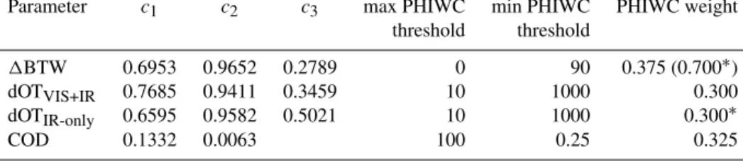
We derive fuzzy logic membership functions for PHIWC based on the magenta curves in Fig. 6. The fits for 1BTW or dOT have the exponential form shown in Eq. (1) whereas the COD is linear as shown in Eq. (2), with x corresponding to the 1BTW, dOT, or COD value, and coefficients c1-c3listed
in Table 2.
TWC = c1·cx2+c3 (1)
TWC = c1·x + c2 (2)
We then linearly rescale the TWC prediction values from Eq. (1) or (2) based on the TWC derived from the Ta-ble 2 maximum (TWCmax)and minimum (TWCmin)PHIWC
Table 2. Coefficients for deriving PHIWC values based on the fits shown by the magenta lines on Fig. 6. 1BTW, COD, and dOT values exceeding the max PHIWC threshold are assigned at PHIWC of 1.0. 1BTW and COD exceeding the min PHIWC Threshold are assigned a PHIWC of 0. Weights for Eq. (4) parameters are indicated in the last column. Weights for Eq. (5) parameters are indicated with an asterisk.
Parameter c1 c2 c3 max PHIWC min PHIWC PHIWC weight
threshold threshold
1BTW 0.6953 0.9652 0.2789 0 90 0.375 (0.700∗) dOTVIS+IR 0.7685 0.9411 0.3459 10 1000 0.300 dOTIR-only 0.6595 0.9582 0.5021 10 1000 0.300∗
COD 0.1332 0.0063 100 0.25 0.325
∗Indicates weight for IR-only PHIWC.
each parameter using Eq. (3): PHIWC(1BTW, dOT, COD) =
TWC-TWCmin
TWCmax−TWCmin
(3) The PHIWC is set to 1.0 for parameter values at or above the maximum threshold. The PHIWC(1BTW or COD) is set to zero for values at or below the minimum threshold because the matched TWC and satellite data show that it is extremely unlikely for HIWC to occur in such warm or optically thin clouds. The PHIWC(dOT) is set to 0.01 for values at or below the minimum threshold because the satellite imagery cannot resolve every OT nor can we detect them all with automated algorithms. A PHIWC(dOT) of zero would produce a final PHIWC of zero using Eqs. (4)–(5) below which would be undesirable.
The final PHIWC value is derived by multiplying the indi-vidual parameter PHIWC values together as shown in Eq. (4) for daytime imagery and Eq. (5) for nighttime imagery:
PHIWCday=PHIWC(1BTW)w1·PHIWC(dOTVIS+IR)w2
·PHIWC(COD)w3 (4)
PHIWCnight=PHIWC(1BTW)w1
·PHIWC(dOTIR-only)w2 (5)
The weights, w1, w2, and w3 defined in Table 2 were
de-rived using an iterative approach to maximize the area un-der the respective PHIWCday and PHIWCnight ROC curves.
1BTW is the highest weighted parameter for PHIWCdaybut
adjusting the weights in favor of another parameter did not appreciably decrease the area under the ROC curve (AUC, discussed in Sect. 3.5). For PHIWCnight, 1BTW has more
weight than dOT. Overall, the difference in AUC for all dif-ferent weight combinations in the night and day products was less than 0.09.
3.4 PHIWC product examples
Examples of the PHIWCnightand PHIWCdayproducts valid
at 23:02 UTC (using the 22:59 UTC MTSAT JAMI scan) dur-ing Flight 22 of the Darwin campaign discussed in Sect. 3.1
are shown in Fig. 2g–h. The aircraft-measured TWC within ±5 min of the image time are overlaid on these graphs, show-ing seven high TWC (magenta X symbols) and other moder-ate TWC observations nearly coincident with this image. The Falcon 20 was flying northwestward toward an area of very cold cloud (1BTW < 5 K). The highest PHIWCnight is
con-centrated near the coldest clouds and IR-only OT detections (Fig. 2c), as would be expected considering that dOT IR-only and 1BTW datasets are used to derive PHIWCnight. Several
high TWC observations were located in ∼ 20 K 1BTW and relatively far (∼ 80 km) from an IR OT detection, combining to generate low (∼ 0.3) PHIWCnight. The VIS image (Fig. 2a)
shows prominent gravity waves emanating away from the OTs to the northwest. Very optically thick cloud (COD > 100) was coincident with all high TWC observations. Addition of these VIS-based products increased the PHIWCdayvalues to
beyond 0.8. There does not seem to be any obvious reason in the satellite-derived products to explain why some mod-erate TWC observations were embedded within a sequence of high TWC observations, again highlighting the challenges in differentiating moderate from high TWC conditions using VIS and IR observations of cloud tops.
The PHIWC time series (Fig. 4d) for Flight 22 of Darwin-2014, described in Sect. 3.1, shows that both the PHIWCday
and PHIWCnight products featured local maxima (> 0.8) at
or near all periods (45 s–8 min duration) when high TWC was observed. These maxima were driven by COD peaks and flight through or near OT and/or textured regions, given that 1BTW was fairly constant throughout the flight. There were many other situations when flights within optically thick clouds and low dOT measured low TWC. As seen in Fig. 2f, areas of high COD can be quite broad and do not al-ways pinpoint the high TWC observed at the −30 to −40◦C flight levels. The dOT product is included in PHIWC to de-pict the proximity to active convective cells that are more likely to generate HIWC conditions. It is very possible that the OT detection products are correctly detecting OTs when low TWC is observed, but the aircraft is upwind of the con-vective core and thus is not observing the high TWC that may be present downwind. The PHIWCdayand PHIWCnight
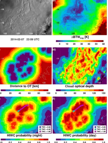
ex-Figure 7. A series of MTSAT-1R JAMI observations and de-rived products for an image during Falcon 20 Flight 16, times-tamped at 23:09 UTC but valid over Australia at 23:12 UTC on 7 February 2014. (a) 0.73 µm VIS reflectance, (b) 1BTW, (c) dOT, (d) smoothed COD, (e) PHIWCnight, and (f) PHIWCday. Panels (e) and (f) are overlaid with 45 s mean TWC observations from 23:07 to 23:17 UTC.
cept around 22:56 UTC, a time very near to that highlighted in Fig. 2. At 22:56 UTC, the nearest IR-only OT detection was ∼ 80 km away (Fig. 4g) with 1BTW near 20 K which combine to reduce PHIWCnight.
An example of the PHIWC products and their inputs are shown in Fig. 7 for an image valid at 23:12 UTC on 7 Febru-ary during Flight 16 of Darwin-2014, also featured in Fig. 1. The Falcon 20 flew very near to or within optically thick (COD > 90) and textured clouds with 1BTW < 5 K 1BTW. Texture and embedded BTW minima were detected well and the aircraft was frequently collocated with dOT < 20 km. Un-like the scene shown in Fig. 2, high COD and texture, low dOT, and extremely cold cloud were collocated, leading to a similar appearance between PHIWCday and PHIWCnight.
High TWC was sustained for much of this flight segment and occurred within areas where PHIWC > 0.9. PHIWC de-creased slightly along the western edge of the segment in conjunction with a decrease to moderate TWC conditions.
Figure 8. Time series of matched aircraft and satellite observations for Flight 16 of Darwin-2014 on 7–8 February 2014. The panels are the same as those described for Fig. 4.
A set of aircraft and satellite product time series for Flight 16 of Darwin-2014 are shown in Fig. 8. The aircraft sam-pled clouds at −40◦C which was about 6 km below cloud top. There were ten individual high TWC encounters during this flight and HIWC conditions persisted for 7–10 min in many of the encounters. PHIWC > 0.8 was present in nine of the ten encounters, with the exception being a twilight high TWC encounter at 22:04 UTC where 1BTW of 13 K and dOT IR-only of 40 km yielded a PHIWC of ∼ 0.4. In gen-eral, the PHIWC time series was highly correlated with TWC except for a high TWC encounter near 22:45 UTC where lower COD (∼ 50), slightly warmer than average 1BTW, and dOT > 20 km combined to produce ∼ 0.6 PHIWC.
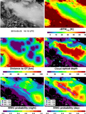
A segment from Falcon 20 Flight 19 of Cayenne-2015 shown in Fig. 9 illustrates an especially challenging case for
satellite-based HIWC detection. The aircraft flew the long segment shown at approximately −12◦C through an anvil
cloud much warmer than those featured in Figs. 2 and 7. The anvil was textured with a few embedded OTs and exhibited high COD. High TWC was observed quite often during the 20 min segment. The PHIWCnightwas extremely low (∼ 0.3)
in high TWC regions due to the relatively warm cloud and lack of distinct BTW minima and IR OT signatures. How-ever, the high COD and texture increased PHIWCdayto
val-ues over 0.75 throughout much of the region where high TWC was observed. This shows the value of VIS-based tex-ture and COD products for capturing HIWC conditions in a cloud which forecasters would not consider to be especially active based on BTW data and spatial patterns alone.
A set of aircraft and satellite product time series for Flight 19 of Cayenne-2015 is shown in Fig. 10. The air-craft sampled clouds at −12◦C (7.1 km) during the first
third of the flight and at −44◦C (11.7 km) for much of
the remainder. There were three (four) high TWC encoun-ters at −12◦C (−44◦C). When the aircraft sampled at −12◦C, TWC was much higher and sustained, on average, than during the rest of the flight. The corresponding values of PHIWCday were also greater, mostly due to high COD
(> 100). The PHIWCday during flight at −44◦C was
corre-lated with TWC but the period of flight spanning 17:20– 17:40 UTC was conducted near the northwest region of the cloud where several new small quasi-isolated cells were ob-served, and consequently, strong gradients in TWC and coin-cident cloud properties are evident in the time series around 17:20, 17:27, and 17:35 UTC. Although the aircraft was very near OTs (dOT < 20 km) at these times, very low TWCs, 1BTW > 30 K, and cloud top heights sometimes below flight level (Fig. 10a) all indicate that the aircraft exited the cloud for brief periods in this region. PHIWCnight was
moder-ated by relatively high 1BTW > 25 K even very near to OTs (dOT < 20 km) and did not exceed 0.70 throughout the en-tire flight. TWC of 1.4 g m−3is an extreme value for 1BTW > 25 K and thus it is impossible to achieve a high PHIWCnight
in these conditions. High TWCs observed at around 18:30 were associated with a different cloud system near Cayenne. Flight 5 on 19 August 2015 during the Florida-2015 cam-paign was observed by GOES-14 during an SRSOR pe-riod, which provided images at 1 min intervals for almost the entire flight. This high temporal resolution GOES-14 im-agery enables precise matches between TWC and satellite products, virtually eliminating matching uncertainties, es-pecially when compared to the 30 min match window used for the GOES-13 data from the Cayenne-2015 campaign. The NASA DC-8 sampled a long-lived but gradually de-caying MCS over Louisiana and offshore regions over the Gulf of Mexico. Time series of the observations and derived products for this flight are shown in Fig. 11. The aircraft flew near the −50◦C level for the first third of the flight and then ranged from the −30 to −50◦C levels for the re-mainder. There were six high TWC periods observed
dur-Figure 9. A series of GOES-13 observations and derived products for an image during Falcon 20 Flight 19 of Cayenne-2015, times-tamped at 16:15 UTC but valid over French Guyana at 16:25 UTC on 23 May 2015. The panels are the same as those described for Fig. 7. The 45 s mean TWC observations are valid from 16:15 to 16:35 UTC.
ing the flight and all of these periods were collocated with PHIWCday≥0.8 and PHIWCnight≥0.6. Flight in dOT
rang-ing from 0 to 20 km generally corresponded with periods of greater TWC. PHIWCday and PHIWCnight were often
con-sistent in magnitude. The exception is the period from 15:10 to 15:40 UTC when the nearest IR-only OT was 30–60 km away but VIS texture was detected within 20 km.
Animations of aircraft TWC observations, satellite obser-vations and products, and the PHIWC products are available at these links (PHIWCday https://satcorps.larc.nasa.gov/
prod/website/yost/2015231/4-panel_VIS+IR/, PHIWCnight
https://satcorps.larc.nasa.gov/prod/website/yost/2015231/ 4-panel_IR/). These animations show that the PHIWC gen-erally evolved quite smoothly due to a combination of the 1 min resolution of the imagery and the inclusion of 1BTW and COD; high values of COD were generally persistent in time. The dOT product induces periodic flickering of high PHIWC that might be considered noise, especially during night when optical depth is not available to constrain the PHIWC product. But it is important to acknowledge that OT
Figure 10. Time series of matched aircraft and satellite observations for Falcon 20 Flight 19 of Cayenne-2015. The panels are the same as those described for Fig. 4.
signatures can be quite short-lived so some PHIWC temporal variability should be expected especially in the vicinity of pulsating updraft regions far removed from other updrafts. Additional animations for Flight 4 on 16 August observed by GOES-14 are also provided at these links to further demonstrate product behavior with this extremely valuable and rare 1 min resolution data. (PHIWCday https://satcorps.
larc.nasa.gov/prod/website/yost/2015228/4-panel_VIS+IR/, PHIWCnight https://satcorps.larc.nasa.gov/prod/website/
yost/2015228/4-panel_IR/). 3.5 PHIWC product validation
The PHIWC products were validated using a simple compar-ison of the probability of detection (POD) and false alarm rate (FAR) for varying PHIWC thresholds. 17:71 nighttime and 15:71 daytime satellite–aircraft matches excluded from
Figure 11. Time series of matched aircraft and satellite observations for Flight 5 of the Florida-2015 campaign on 19 August 2015. The panels are the same as those described for Fig. 4.
product training (see Sect. 2.4) were used for validation. As noted in Sect. 3.3, given that the satellite parameters show reduced sensitivity to TWC for moderate TWC values (> 0.5 g m−3), we use 0.5 g m−3to define a correct detection but we will also discuss results relative to the more realistic HIWC TWC threshold of 1.0 g m−3.
The ROC curves shown in Fig. 12 were constructed by plotting POD and FAR for thresholds chosen at intervals of 0.05 within the range 0–1.0. The thresholds are labeled at intervals of 0.1 along each curve. ROC curves using both 0.5 and 1.0 g m−3 to define high TWC events requiring de-tection are shown in top and bottom panels, respectively, of Fig. 12. A ROC curve for a perfect PHIWC product would in-tercept the (0.0, 1.0) coordinate and the area under the curve (AUC) would equal 1.0. The PHIWC threshold nearest the (0.0, 1.0) coordinate can be considered the optimal
thresh-old because it yields the best compromise between POD and FAR. Therefore AUC was used as a metric to quantify the skill of the PHIWC product, and the optimal PHIWC thresh-old was identified based on maximum AUC. For PHIWCday,
(solid black curve) the optimal PHIWC threshold is 0.70 and yields a 75 % POD and 35 % FAR based on the 0.5 g m−3 threshold. This is consistent with the flight track time series results where a PHIWCday> 0.70 regularly identified high
TWC events. The optimal threshold for PHIWCnight (solid
gray curve) is 0.55 and yields a 60 % POD and 32 % FAR. The PHIWCnight POD would be 62 % to achieve the same
35 % FAR as the optimal PHIWCdayproduct. FAR would
de-crease by up to 10 % if a lower TWC threshold such as 0.01– 0.05 g m−3were used to define cloud because the satellite-observed characteristics of clouds with such low TWC rarely triggers high PHIWC. But it is felt that 0.1 g m−3 provides the most reliable detection of cloud boundaries and that statistics using this threshold are most representative of true product performance, keeping in mind the challenges associ-ated with validation described below.
The reduction of skill for PHIWCnight is not especially
surprising given Fig. 6 that showed a relatively wide range of IR-only dOT and 1BTW for TWC > 0.5 g m−3. Lower PHIWCnight values on average also reflect this uncertainty.
The combination of these IR-based fields with COD and es-pecially VIS texture detection more precisely depicts where HIWC is likely than the IR-based fields alone. In the event that a COD retrieval product is unavailable due to latency constraints, VIS OT and texture can be combined with IR OT detection to derive dOT and an alternative two-parameter PHIWCday product. Based on TWC > 0.5 g m−3, this
al-ternative two-parameter PHIWCday (Fig. 12, dashed black
curve) would provide a 6 % reduction in POD relative to the three-parameter PHIWCdaybut a 7 % improvement over the
PHIWCnightfor a constant 35 % FAR.
If HIWC conditions are defined as TWC > 1.0 g m−3rather than TWC > 0.5 g m−3 the accuracy of PHIWC is affected very little. The maximum AUC changes only slightly for all three PHIWC versions. A higher PHIWC threshold is re-quired to discriminate the 1.0 g m−3TWC events; for exam-ple, the optimal PHIWCdaythreshold is 0.75 (versus 0.70 for
0.5 g m−3)which yields a 75 % POD and 37 % FAR. A comparison of the PHIWC distribution for varying TWC intervals is shown in Fig. 13. In general, both PHIWCday and PHIWCnight increase as a function of TWC
up to a value of 1.0 g m−3but then level off at high PHIWC values in HIWC conditions. Very high TWC (> 2 g m−3, 95th percentile in this 45 s dataset) seldom occurs when PHIWCday< 0.7 and PHIWCnight < 0.4 during Florida-2015
and Darwin-2014 campaigns. Cayenne-2015 featured sev-eral cases of low PHIWCnightin very high TWC conditions,
perhaps driven by the coarse 30 min GOES sampling that cannot always capture rapidly evolving OTs or cold cloud tops signifying HIWC conditions. The Cayenne-2015 cam-paign featured the lowest PHIWC on average due to the
Figure 12. A receiver operating characteristic (ROC) curve show-ing the relationship between POD and FAR for PHIWC thresholds ranging from 0.0 to 1.0 (labeled at 0.1 increments) based on TWC thresholds of 0.5 g m−3(a) and 1.0 g m−3(b). The solid black curve represents the three-parameter PHIWCdayand the solid grey curve
represents the two-parameter PHIWCnight. The dashed black curve
represents an algorithm formulation using 1BTW and dOT analo-gous to PHIWCnight, but VIS OT and texture detections in addition
to IR OT detections are used to derive dOT. This formulation could be used for daytime HIWC detection in the event that a COD re-trieval product is unavailable. Optimal PHIWC values based on the maximum area underneath the ROC curve (AUC) are circled and the corresponding AUC is provided in the legend.
fact that clouds had the warmest cloud tops and greatest 1BTW. There are many instances of low PHIWCnight but
higher PHIWCday in HIWC conditions, further
demonstrat-ing the importance of COD and VIS dOT. Challenges associ-ated with PHIWC validation are discussed in the next section
Figure 13. Box and whisker diagrams showing the relationship between PHIWCday (top, N = 4598 satellite–aircraft matches),
PHIWCnight (bottom, N = 5371) and TWC. The rectangles show the intraquartile PHIWC range for each TWC bin. The horizontal line within the rectangles shows the median PHIWC. The whiskers show the range of the 1.5 and 98.5 % of the distribution and circles are outliers.
that could help to explain perceived deficiencies in the prod-ucts.
One point to consider when interpreting these results is that 45 s TWC data was used to develop and validate the TWC algorithms, not the native 5 s data. Though 45 s data is more representative of the size of a 2 × 2 GEO pixel clus-ters co-located with the aircraft than 5 s, averaging across the 45 s window dampens mesoscale variability that could contribute to temperatures and spatial patterns observed by satellite, especially texture in 1 km VIS imagery that is 16 times finer than 4 km IR BT. For example, the PHIWCday
threshold of 0.70 featured a 35 % FAR based on 45 s data. 41 % of these false positives featured a 5 s TWC > 0.5 g m−3 and 1.0 % featured TWC > 1.0 g m−3. Of course the true pos-itive rate would almost certainly decrease if, for example, 5 s TWC > 0.5 g m−3required high PHIWC. Thus, there are both pros and cons regarding the use of 5 versus 45 s TWC data that complicate validation, but it is felt that the PHIWC algo-rithm based on 45 s data is robust.
During the Darwin-2014 and Cayenne-2015 campaigns, the 95 GHz Doppler Radar System Airborne (RASTA, Pro-tat et al., 2009) provided vertical TWC profiles above and below the aircraft that can be used to estimate if false detec-tions from the PHIWC products based on comparison with IKP2 were truly false, namely there were no retrievals of
TWC ≥ 0.5 g m−3 anywhere within the column. TWC ob-served during the flight campaigns decreased with height by 33 % from the −10◦C layer to the −30 to −50◦C layer. If
the aircraft was flying at −50◦C and measured 0.4 g m−3, TWC could exceed 0.5 or possibly 1.0 g m−3at lower alti-tudes in the same column. Moderate to high TWC at low to mid-levels could be correlated with cold and/or textured cloud tops that would trigger high PHIWC values. Flight-level RASTA TWC retrievals were found to have a ∼ 10– 30 % bias and 40–70 % root-mean-squared difference rela-tive to in situ TWC measurements during the Darwin-2014 campaign (Protat et al., 2016). Although RASTA TWC esti-mates remote from the aircraft level have not yet been val-idated for accuracy, the radar TWC retrievals were consid-ered to be adequate to analyze for the following false de-tections (Protat et al., 2016). A FAR of 31 % was found for 0.7 PHIWCdayfor Darwin-2014 and Cayenne-2015 based on
a 0.5 g m−3IKP2 threshold. 82 % (35 %) of the false detec-tions were collocated with RASTA column-maximum TWCs that exceeded 0.5 (1.0) g m−3at heights above the freezing level. This suggests that vertical sampling bias, especially when the aircraft flew at higher flight levels where TWC is lower on average, is likely influencing the IKP2-based vali-dation statistics and therefore these statistics may not be truly representative of product performance.
On the other hand, when column-max RASTA TWC is used as truth for Darwin-2014 and Cayenne-2015, a nearly identical shape of the ROC curves relative to those from IKP2 (not shown) was found. When the column-maximum RASTA TWC is analyzed in conjunction with the satellite parameters used to derive PHIWC, very similar relationships are found with those shown in Fig. 6 which would lead to comparable RASTA-based PHIWC. So while some per-haps appreciable fraction of the false detection rate can be explained by vertical variability and sampling bias, use of RASTA data is not enabling significant improvement in over-all PHIWC accuracy.
4 Discussion
Our analysis found that HIWC conditions are most com-mon during periods of flight within or beneath optically thick cloud tops having temperatures near to or colder than the tropopause and within 40 km of an OT or textured cloud top. A combination of VIS-based texture detection and COD re-trieval helps to pinpoint where HIWC conditions are likely within or beneath a broad area of cold anvil. High COD indicates a cloud top composed of dense ice which gener-ates high VIS reflectance. The Reffshowed a nearly identical
distribution in moderate and high TWC conditions, so the high COD and VIS reflectance is driven either by a high ice mixing ratio in anvil clouds without deep convection under-neath or by large vertical cloud thickness, i.e., the presence of deep convection. Convective updrafts depicted by OT