Regional reference total electron content model over Japan based on neural network mapping techniques

HAL Id: hal-00318425

https://hal.archives-ouvertes.fr/hal-00318425

Submitted on 2 Jan 2008

HAL is a multi-disciplinary open access

archive for the deposit and dissemination of

sci-entific research documents, whether they are

pub-lished or not. The documents may come from

teaching and research institutions in France or

abroad, or from public or private research centers.

L’archive ouverte pluridisciplinaire HAL, est

destinée au dépôt et à la diffusion de documents

scientifiques de niveau recherche, publiés ou non,

émanant des établissements d’enseignement et de

recherche français ou étrangers, des laboratoires

publics ou privés.

Regional reference total electron content model over

Japan based on neural network mapping techniques

T. Maruyama

To cite this version:

T. Maruyama. Regional reference total electron content model over Japan based on neural network

mapping techniques. Annales Geophysicae, European Geosciences Union, 2008, 25 (12), pp.2609-2614.

�hal-00318425�

www.ann-geophys.net/25/2609/2007/ © European Geosciences Union 2007

Annales

Geophysicae

Regional reference total electron content model over Japan based on

neural network mapping techniques

T. Maruyama

National Institute of Information and Communications Technology, 2-1 Nukuikita 4-chome, Koganei, Tokyo, 184-8795 Japan Received: 26 July 2007 – Accepted: 27 November 2007 – Published: 2 January 2008

Abstract. A regional reference model of total electron con-tent (TEC) was constructed using data from the GPS Earth Observation Network (GEONET), which consists of more than 1000 Global Positioning System (GPS) satellite re-ceivers distributed over Japan. The data covered almost one solar activity period from April 1997 to June 2007. First, TECs were determined for 32 grid points, expanding from 27 to 45◦_{N in latitude and from 127 to 145}◦_{E in longitude}

at 15-min intervals. Secondly, the time-latitude variation av-eraged over three days was determined by using the surface harmonic functional expansion. The coefficients of the ex-pansion were then modeled by using a neural network tech-nique with input parameters of the season (day of the year) and solar activity (F10.7 index and sunspot number). Thus, two-dimensional TEC maps (time vs. latitude) can be ob-tained for any given set of solar activity and day of the year.

Keywords. Ionosphere (Mid-latitude ionosphere; Modeling and forecasting; Instruments and techniques)

1 Introduction

One of the important effects of the ionosphere on radio waves is a propagation delay in the ionosphere. This delay de-pends on the frequency and the total electron content (TEC) along the propagation path. Several attempts have been made to specify the ionospheric electron density using theoretical (see Anderson et al., 1998) and empirical approaches. Con-siderable effort has resulted in the continuous development and improvement of the International Reference Ionosphere (IRI) (Bilitza, 2001), which describes the density at various heights for any specified geophysical conditions, based on long-term observations. TEC can be derived by integrating

Correspondence to: T. Maruyama

(tmaru@nict.go.jp)

the height profile of the electron density. The contribution of the plasmaspheric electron density to TEC cannot be ne-glected (Gulyaeva and Titheridge, 2006; Gulyaeva and Gal-lagher 2007; Cueto et al., 2007; Reinisch et al., 2007). How-ever, observations of the electron density to construct a reli-able model are limited in the topside ionosphere and plasma-sphere compared with the bottomside and the F-layer peak (Bilitza and Williamson, 2000).

Direct measurements of TEC using radio waves transmit-ted from the Global Positioning System (GPS) satellites have been collected in this decade. Thus, GPS-based TEC data are now available to construct empirical models of TEC. Mean-while, artificial neural network (NN) techniques have been applied to a variety of topics in the study of the upper at-mosphere. Multilayer feed-forward networks (Rumelhart et al., 1986; Haykin, 1994) are used to specify the ionosphere by approximating a relationship between geophysical condi-tions (seasons, solar activities, local times, longitude/latitude etc.) and observed ionospheric parameters (foF2, h’F2,

hmF2, etc.) (Williscroft and Poole, 1996; McKinnell and

Poole, 2004; Oyeyemi et al., 2005), short-term forecasting of ionospheric conditions (Altinay et al., 1997; Cander et al., 1998; Kumluca et al., 1999; Wintoft and Cander, 2000; Poole and McKinnell, 2000; Oyeyemi et al., 2006), and long-term trend analyses (Poole and Poole, 2002; Yue et al., 2006). Because of the input-output mapping features of NNs, they could be used to generate reference ionospheric models for possible incorporation into the IRI (McKinnell and Friedrich, 2007). For this purpose, a so-called training data set must cover a whole range of possible input parameter variations, say, a data period longer than one solar cycle.

In Japan, a dense GPS receiver network, GEONET (GPS Earth Observation Network) has been developed, and data from more than 1000 locations have been available since April 1997, close to a solar minimum. An algorithm that simultaneously determines satellite/receiver biases and verti-cal TEC using GEONET data has been developed by Ma and

2610 T. Maruyama: Regional reference total electron content model 130 135 140 145 45 40 35 30 25 Longitude (deg. E) Latitude (deg. N)

Fig. 1. 32 grid points on which TECs were determined at 15-min intervals. 400 300 200 100 0

Solar Flux (sfu)

300 200 100 0 Sunspot Number F10.7 R 1997 1998 1999 2000 2001 2002 2003 2004 2005 2006 2007 Year

Fig. 2. Observed daily solar flux (upper trace with left scale) and daily sunspot number (lower trace with right scale) from April 1997 to June 2007.

Maruyama (2003). By using this algorithm, we constructed a TEC database that nearly covered one solar cycle from 1997 to 2007.

The data set used to develop the regional reference TEC model and the NN technique are described in Sect. 2. The performance of the trained network is evaluated in Sect. 3. Section 4 summarizes the work.

2 Data set and methodology

About 300 GEONET receivers were chosen for this study to ensure uniform coverage over Japan. The major issues in deriving TECs from GPS radio signal observations are the instrumental biases both in the satellites and receivers, and the conversion process from the observed TECs along the slant path to the vertical ones. In this paper, the slant TECs were converted to vertical TECs (vTEC) at the piercing point where the ray path crossed a shell at a height of 400 km (thin shell model). Assuming that the vTECs in a small cell 2×2◦

in longitude and latitude were the same in a short period of time, we calculated the daily instrumental biases and vTEC in each cell with a 15-min period, using the least-squares fit-ting method for a data set that covered 24 h. More details of the method are described elsewhere (Ma and Maruyama, 2003). The vertical TEC obtained in this way is referred to as the grid TEC (gTEC). The original TEC grid consisted of 32 grids, as shown in Fig. 1 (the southern most two grids were not used when constructing the actual model because gaps of a few hours in the data occurred, depending on the change in the satellite constellation).

The major factors that determine the TEC are the solar activity, season, local time, and geographic and geomag-netic coordinates. Our process to generate a model con-sists of three steps: Step 1 is the procedure described in the previous paragraph in which the gTECs at the grid points are determined at 15-min intervals. Step 2 is the procedure where variations in time and latitude are expressed as a two-dimensional distribution map for three consecutive days. Be-cause the data grid is limited to a narrow longitudinal extent and geomagnetic conditions do not change greatly among the east-west aligned grids, the longitudinal dependence is as-sumed to be equivalent to the local mean time (LMT) in this step. Step 3 is the procedure where the solar activity and sea-sonal changes in the TEC map are modeled by using a neural network technique.

To generate TEC maps from the gTECs, we used the surface harmonic expansion method based on the associ-ated Legendre function, as shown in (1), taking the LMT (hour) at each grid point as the azimuth parameter, i.e. φ = 2π(LMT/24), TEC = M X m=0 N X n=m

(Anmcos mφ + Bnmsin mφ)Pnm(cos θ ), (1)

where θ is the colatitude; we took the degree and order up to 7 (N =M=7). As the grid point distributes at only northern mid-latitudes, dummy data were set, for mathematical conve-nience, in the Southern Hemisphere as a mirror image of the Northern Hemisphere with respect to the equator. The func-tional fitting was performed to determine coefficients Anm

and Bnm in (1). As dummy data were set in the Southern

Hemisphere, the whole global distribution map is symmetri-cal with respect to the equator (resultant map data outside the

latitude range from 29 to 45◦_{N were disregarded). In other}

words, Anmand Bnmwith the odd number of n+m are equal

to zero. Thus, a total of 36 target parameters needed to be determined.

The solar activity expressed by two proxies, the F10.7 so-lar flux (sfu = 10−22_{W m}−2_Hz−1_{) and the sunspot number,}

R, for the whole data period is shown in Fig. 2. The figure shows that both proxy parameters vary in a similar way but are not exactly the same. For example, from the latter half of 2001 to 2002, the solar flux reached a maximum, but the sunspot number reached a maximum in 2000. Thus, both parameters were included in the input parameters of the net-work. To successfully separate the seasonal and solar activity dependence of the TEC after training a neural network, the combination of both parameters must be homogeneously dis-tributed in the training data set. Figure 3 shows the seasonal distribution of the solar activity proxies from 1997 to 2007, which indicates a homogeneous distribution in the range be-tween 75 and 200 for F10.7 and bebe-tween 0 and 150 for R. Within this range, a neural network is expected to separate the seasonal and solar activity dependence of the TEC.

We adopted the multilayer feed-forward network (Rumel-hart et al., 1986; Haykin, 1994) that consisted of the input layer, one hidden layer, and the output layer. The schematic diagram of the network is shown in Fig. 4. The input layer had 8 nodes for solar activity (F10.7 and R averaged over three days, a week, and three solar rotations (81 days), in-cluding the days in which the TEC was specified and prior to those days) and season (sin and cos components of day of the year). The number of nodes in the hidden layer was chosen to be 200. The output parameters were the 36 Leg-endre coefficients, as described in this section. For the first several tenths of the epochs in the back-propagation learning process, weight updating was performed by the pattern mode in which weights were updated after the presentation of each training example (Haykin, 1994). The order of the presenta-tion of training examples was randomized from one epoch to the next. After the weights were coarsely determined, weight updating was continued by the batch mode in which weights were updated after the presentation of all the training exam-ples that constituted an epoch (Haykin, 1994).

3 Results

To evaluate the performance of the neural network mapping, we ran the network learning for the data set, excluding a par-tial data set for 2003. After the learning was completed, the network outputs were compared with observations for 2003. The results for the four typical seasons are shown in Figs. 5 to 8. The upper panel of Fig. 5 is the TEC distribution map (local mean time vs. latitude) for the March equinox 2003, reconstructed using the coefficient vector predicted by the network. The lower panel of Fig. 5 is the mean TEC dis-tribution map generated using observations over the 27-day

400 300 200 100 0

Solar Flux (sfu)

300

200

100

0

Sunspot Number

Jan Feb Mar Apr May Jun Jul Aug Sep Oct Nov Dec Month

F10.7

R April 1997 - June 2007

Fig. 3. Seasonal distribution of observed daily solar flux (upper panel) and daily sunspot number (lower panel) from April 1997 to June 2007. F10.7 [3] F10.7 [7] F10.7 [81] R [3] R [7] R[81] Input layer (8 nodes) Hidden layer (200 nodes) Output layer (36 nodes) cos

(

(

)

Fig. 4. Schematic diagram of NN. For solar activity indices, [n] denotes an average over n days.

period centered on 21 March 2003. These two panels resem-ble each other very well, even though the observed values (lower panel) are slightly higher than the predicted values (upper panel). The diurnal maxima are at around 13:00 LT at the lowest latitude (29◦_{N) and at around 12:30 LT at the}

highest latitude (45◦_{N) in both maps. Also, a small bulge in}

the contour near sunset at latitudes 35–40◦_{N is common in}

2612 T. Maruyama: Regional reference total electron content model 40 35 30 25 25 20 20 15 15 10 10 21 March 2003 45 40 35 30 30 25 25 20 20 15 15 10 10 40 30 20 10 45 40 35 30 45 40 35 30 24 21 18 15 12 9 6 3 0 Local Time (hr) TEC unit Latitude (deg. N) (a) (b) 45

Fig. 5. Local time-latitude distribution of TEC; (a) predicted by trained NN for March equinox in 2003 and (b) mean TEC averaged over a 27-day period centered on March equinox 2003 constructed using gTEC data.

25 20 15 15 15 22 June 2003 25 20 15 15 40 30 20 10 45 40 35 30 45 40 35 30 24 21 18 15 12 9 6 3 0 Local Time (hr) TEC unit Latitude (deg. N) (a) (b)

Fig. 6. Same as Fig. 5 but for June solstice 2003.

Figure 6 is the same as Fig. 5, except for the June sol-stice. The two maps have quite similar diurnal and latitudinal patterns and absolute TEC values. A distinct feature of this season was the formation of three diurnal peaks of TEC and a small day-night difference. The morning peaks are cen-tered at 07:30 LT in both maps, even though the amplitude is small for the observed 27-day means (lower panel). The times of the afternoon peaks shifted slightly earlier in the network predicted map (upper panel) than in the observed map. However, their trend of an earlier appearance at higher latitudes is common in both maps. The times of the evening peaks are almost the same for both maps. Figures 7 and 8 are the same as Fig. 5, but they are for the September equinox and the December solstice, respectively. In these figures, the network predicted (upper panels) and the observed (lower panels) maps are very similar in many features and absolute values. 30 25 20 15 15 ₁₀ 10 10 23 September 2003 30 25 20 15 15 10 10 40 30 20 10 45 40 35 30 45 40 35 30 24 21 18 15 12 9 6 3 0 Local Time (hr) TEC unit Latitude (deg. N) (a) (b)

Fig. 7. Same as Fig. 5 but for September equinox 2003.

25 20 15 15 10 10 5 5 5 5 22 December 2003 25 20 15 15 10 10 5 5 5 40 30 20 10 45 40 35 30 45 40 35 30 24 21 18 15 12 9 6 3 0 Local Time (hr) TEC unit Latitude (deg. N) (a) (b)

Fig. 8. Same as Fig. 5 but for December solstice 2003.

For more comparisons, the TECs at noon at grid point 14 (35◦_{N, 137}◦_{E) near central Japan, as denoted by the asterisk}

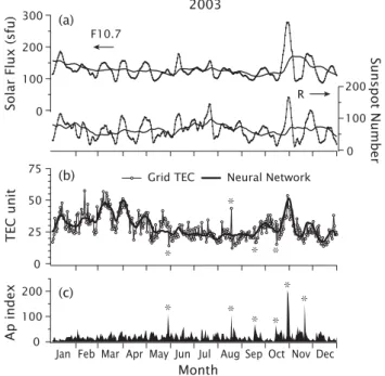
in Fig. 1, were calculated and are shown in Fig. 9. The top panel is the solar activity inputs, F10.7 (upper traces) and R (lower traces), averaged over three days (dots connected with thin lines) and three solar rotations (solid lines). The middle panel is the grid TECs (circles connected with thin line) and network outputs (thick solid line). Not only seasonal varia-tions, but also solar activity dependences are reproduced by the network. Interestingly, at the end of October, the solar flux was quite large, but the grid TEC did not increase very much. This was well reproduced by the network. When the solar activity indices averaged over three solar rotations were not incorporated into the input parameter, this moderate in-crease in TEC against the extremely intense solar activity at the end of October was not successfully reproduced. On the other hand, the enhanced grid TEC found in the latter half of May was not reproduced by the network. In this period, the solar activity was not so high as compared with the so-lar activity in the soso-lar rotation before and after this period.

300 200 100 0

Solar Flux (sfu)

200 100 0 Sunspot Number 75 50 25 0 TEC unit

Grid TEC Neural Network F10.7

R 2003

Jan Feb Mar Apr May Jun Jul Aug Sep Oct Nov Dec Month 200 100 0 Ap index (a) (b) (c)

Fig. 9. (a) Solar activity variation of three-day mean (dots con-nected with line) and 81-day mean (solid lines) for 2003. (b) Com-parison of TEC predicted by NN and gTEC at grid number 14 (35◦_{N, 137}◦_{E), 12:00 LT. (c) Ap index. The Ap index was not}

incorporated into the input parameter.

This suggests that the solar activity indices we used are not entirely accurate proxies of solar EUV flux.

In our model, TEC variations associated with magnetic storms were not considered, while magnetic activities largely affect values of TEC. Discrepancy between the observed TECs and network predictions, as seen in the middle panel of Fig. 9, could be partly due to TEC variations caused by mag-netic storms. The bottom panel of Fig. 9 shows the Ap index. Corresponding to the geomagnetic disturbances on 29 May, 17 September, 14 October, the observed TEC values nega-tively departed from the network predictions, as denoted by the asterisks. While on 18 August, the observed TEC value was much larger than the network prediction. On the other hand, the two largest storms on 29 October (the Halloween storm) and 20 November did not cause large TEC distur-bances in the Japan’s sector. In the February–April period, no clear correspondence was found between the large TEC discrepancy and magnetic disturbances. Thus the Ap index alone is not sufficient to predict storm effects on TEC, and incorporating storm effects into the model is a future prob-lem.

Total performance of the constructed model over a year is shown in Fig. 10. The left panel is a scatter diagram of the hourly values of the network outputs for grid number 14 (35◦_{N, 137}◦_{E) against corresponding TECs obtained from a}

data set similar to that used in network training, i.e. spherical harmonic functional fitting of three consecutive days (step

50

0

50 0

Fitted TEC (TEC unit)

NN outputs (TEC unit)

(a) RMSE=3.29 TEC unit (b) 50

0

50 0

gTEC (TEC unit)

NN outputs (TEC unit)

RMSE=4.52 TEC unit

Fig. 10. Total performance of NN prediction. Scatter plots of NN-predicted hourly TEC for 2003 vs. TEC after functional fitting (a) and grid TEC before functional fitting (b).

2) in 2003. Thus, this gives the performance of network learning only (step 3). In this comparison, the root mean square error (RMSE) was 3.29 TEC units. The right panel is a scatter diagram of the predicted hourly values against the grid TEC (step 1) at the same grid point. The RMSE is slightly higher than that for the functional fitting results and was 4.52 TEC units, because the functional fitting averaged unpredictable day-to-day variability, including magnetic dis-turbance effects, over three days.

4 Summary

A large amount of GPS-derived total electron content data has been collected in this decade covering almost one solar cycle, which now allows for an empirical model of TEC to be constructed. We constructed a regional reference TEC model over Japan based on the dense GPS receiver network, GEONET. The process consisted of three steps: (1) deter-mining vertical TECs at grid points separated by 2◦ _in

lat-itude and longlat-itude (gTECs), (2) approximating by using surface harmonic functional fitting (time-latitude maps), and (3) using neural network mapping to relate the solar activ-ity and season with the pattern of the time-latitude map. In the first step, instrumental biases were simultaneously deter-mined and vTECs were averaged in 2×2◦_{longitude/latitude}

cells. Averaging and smoothing were also performed in step 2 by using limited degree and order of the surface harmonic function to approximate gTEC over three days. Step 3 suc-cessfully worked to separate the solar activity and seasonal dependences of the TEC distribution pattern with respect to time and latitude.

Acknowledgements. GEONET is operated by the Geographical

Survey Institute, Japan, and data in RINEX format were obtained from the Japan Association of Surveyors (JAS).

Topical Editor M. Pinnock thanks two anonymous referees for their help in evaluating this paper.

2614 T. Maruyama: Regional reference total electron content model References

Altinay, O., Tulunay, E., and Tulunay, Y.: Forecasting of iono-spheric critical frequency using neural networks, Geophys. Res. Lett., 24, 1467–1470, 1997.

Anderson, D. N., Buonsanto, M. J., Codrescu, M. et al.: Intercom-parison of physical models and observations of the ionosphere, J. Geophys. Res., 103, 2179–2192, 1998.

Bilitza, D.: International Reference Ionosphere 2000, Radio Sci., 36, 261–275, 2001.

Bilitza, D. and Williamson, R.: Towards a better representation of the IRI topside based on ISIS and Alouette data, Adv. Space Res., 25(1), 149–152, 2000.

Cander, L. R., Milosavljevic, M. M., Stankovic, S. S., and Toma-sevic, S.: Ionospheric forecasting technique by artificial neural network, Electronics Lett., 34, 1573–1574, 1998.

Cueto, M., Co¨ısson, P., Radicella, S. M., Herraiz, M., Ciraolo, L., and Brunini, C.: Topside ionosphere and plasmasphere: Use of NeQuick in connection with Gallagher plasmasphere model, Adv. Space Res., 39, 739–743, 2007.

Gulyaeva, T. L. and Titheridge, J. E.: Advanced specification of electron density and temperature in the IRI ionosphere-plasmasphere model, Adv. Space Res., 38, 2587–2595, 2006. Gulyaeva, T. L. and Gallagher, D. L.: Comparison of two IRI

electron-density plasmasphere extensions with GPS-TEC obser-vations, Adv. Space Res., 39, 744–749, 2007.

Haykin, S.: Neural networks – A comprehensive foundation, Macmillan College Publishing Company, Inc., 1994.

Kumluca, A., Tulunay, E., Topalli, I., and Tulunay, Y.: Temporal and spatial forecasting of ionospheric critical frequency using neural networks, Radio Sci., 34, 1497–1506, 1999.

Ma, G. and Maruyama, T.: Derivation of TEC and estimation of instrumental biases from GEONET in Japan, Ann. Geophys., 21, 2083–2093, 2003,

http://www.ann-geophys.net/21/2083/2003/.

McKinnell, L. A. and Friedrich, M.: A neural network-based iono-spheric model for the auroral zone, J. Atmos. Sol.-Terr. Phy., 69, 1459–1470, 2007.

McKinnell, L. A. and Poole, A. W. V.: Predicting the ionospheric F layer using neural networks, J. Geophys. Res., 109, A08308, doi:10.1029/2004JA010445, 2004.

Oyeyemi, E. O., Poole, A. W. V., and McKinnell, L. A.: On the global model for foF2 using neural networks, Radio Sci., 40, RS6011, doi:10.1029/2004RS003223, 2005.

Oyeyemi, E. O., McKinnell, L. A., and Poole, A. W. V.: Near-real time foF2 predictions using neural networks, J. Atmos. Sol.-Terr. Phy., 68, 1807–1818, 2006.

Poole, A. W. V. and McKinnell, L. A.: On the predictability of foF2 using neural networks, Radio Sci., 35, 225–234, 2000.

Poole, A. W. V. and Poole, M.: Long-term trends in foF2 over Gra-hamstown using neural networks, Ann. Geophys., 45, 155–161, 2002,

http://www.ann-geophys.net/45/155/2002/.

Reinisch, B. W., Nsumei, P., Huang, X., and Bilitza, D. K.: Model-ing the F2 topside and plasmasphere for IRI usModel-ing IMAGE/RPI and ISIS data, Adv. Space Res., 39, 731–738, 2007.

Rumelhart, D. E., Hinton, G. E., and Williams, R. J.: Learning rep-resentations by back-propagating errors, Nature, 323, 533–536, 1986.

Williscroft, L. A. and Poole, A. W. V.: Neural networks, foF2, sunspot number and magnetic activity, Geophys. Res. Lett., 23, 3659–3662, 1996.

Wintoft, P. and Cander, L. R.: Twenty-four hour predictions of foF2 using time delay neural networks, Radio Sci., 35, 395–408, 2000. Yue, X., Wan, W., Liu, L., Ning, B., and Zhao, B.: Applying ar-tificial neural network to derive long-term foF2 trends in the Asia/Pacific sector from ionosonde observations, J. Geophys. Res., 111, A10303, doi:10.1029/2005JA011577, 2006.