Sulfur and nitrogen levels in the North Atlantic Ocean's atmosphere: A synthesis of field and modeling results

HAL Id: hal-02875493

https://hal.archives-ouvertes.fr/hal-02875493

Submitted on 3 Feb 2021

HAL is a multi-disciplinary open access

archive for the deposit and dissemination of

sci-entific research documents, whether they are

pub-lished or not. The documents may come from

teaching and research institutions in France or

abroad, or from public or private research centers.

L’archive ouverte pluridisciplinaire HAL, est

destinée au dépôt et à la diffusion de documents

scientifiques de niveau recherche, publiés ou non,

émanant des établissements d’enseignement et de

recherche français ou étrangers, des laboratoires

publics ou privés.

Sulfur and nitrogen levels in the North Atlantic Ocean’s

atmosphere: A synthesis of field and modeling results

J. Galloway, J. Penner, C. Atherton, J. Prospero, H. Rodhe, R. Artz, Yves

Balkanski, H. Bingemer, R. Brost, S. Burgermeister, et al.

To cite this version:

J. Galloway, J. Penner, C. Atherton, J. Prospero, H. Rodhe, et al.. Sulfur and nitrogen levels in the

North Atlantic Ocean’s atmosphere: A synthesis of field and modeling results. Global Biogeochemical

Cycles, American Geophysical Union, 1992, 6 (2), pp.77-100. �10.1029/91GB02977�. �hal-02875493�

GLOBAL BIOGEOCHEMICAL CYCLES, VOL. 6, NO. 2, PAGES 77-100, JUNE 1992

ATLANTIC OCEAN'S ATMOSP•RE- A SlrgrHBSIS OF

FIELD AND MODELING RESULTS

•.N. Galloway, 1 •.E. Penner,

2 C.S. Atherton, 2

•.M. Prospero,

3 H. Rodhe,

4 R.S. Artz, 5

Y.•. Balkanski,

6 H.G. Bingemet,

7 R.A. Brost, 8

S. Burgermeister, 9 G.R. Carmichael, 10

•.S. Chang,

11 R.•. Charlson,

12 S. Cober,

13

W.G. Ellis,

•r., 14 C.•. Fischer, 15

•.M. Hales, 16 D.R. Hastie, 17 T. Iversen, 18

D.•. •acob, 6 œ. •ohn, 10 •.E. •ohnson,

19

P.S. Kasibhatla, 20 •. Langner,

4

•. Lelieveld, 8 H. Levy 11, 20 F. Lipschultz, 21

•.T. Merrill, 14 A.F. Michaels, 21

•.M. Miller, 5 •.L. Moody,

1 •. Pinto, 22

A.A.P. Pszenn•,

15 P.A. Spiro,

6 L. Tarfason,

18

S.M. Turner, 2• and D.M. Whelpdale

24

1University of Virginia, Charlottesville.

2Lawrence

Livermore

National Laboratory,

Livermore, California.

3RSMAS,

University of Miami, Miami,

Florida.

4University of Stockholm, Stockholm.

5NOAA

Air Resources

Laboratory, Silver

Spring, Maryland.

6Harvard

University, Cambridge,

Massachusetts.

7Max Planck Institute for Chemistry, Mainz,

Germany.

8Max

Planck Institute for Chemistry, Mainz,

Germany.

9Goethe

University, Frankfurt, Germany.

10University of Iowa, Iowa City.

11State University of New

York, Albany.

12University of Washington, Seattle.

13University of Toronto, Toronto, Canada.

14University of Rhode

Island, Narragansett.

15NOAA

Atlantic Oceanographic

and Meteoro-

logical

Laboratory,

Miami,

Florida.

17york University, North York, Canada.

18The Norwegian

Meteorology Institute, Oslo.

19NOAA

Pacific Marine Environmental Labo-

20NOAA

Geophysical

Fluid Dynamics

Labora-

21Bermuda

Biological Station for Research,

22Environmental

Protection Agency, Research

23University of East Anglia, Norwich,

Enõland.

2•Atmospheric

Environment

Service, Downs-

view, Canada.

Copyright 1992

by the American Geophysical Union.

Paper number 91GB0297 7. 0886-6236 / 92/91GB-0297 7 810.00

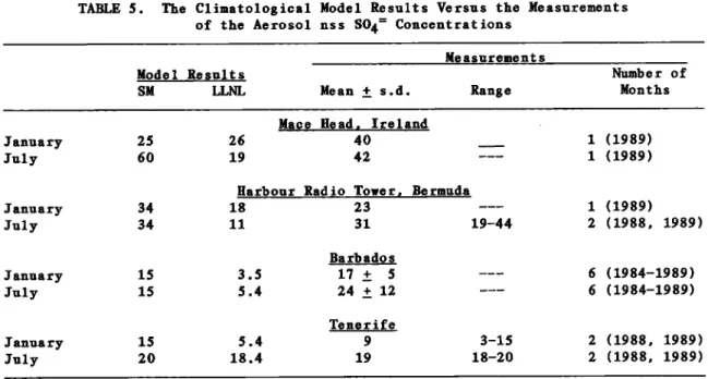
Abstract. In April 1990, forty-two

scientists from eight countries attended

a workshop at the Bermuda Biological Station for Research to compare field

measurements with model estimates of the

distribution and cycling of sulfur and

nitrogen species in the North Atlantic Ocean's atmosphere. Data sets on hori-

zontal and vertical distributions of

sulfur and nitrogen species and their rates of deposition were available from ships' tracks and island stations.

These data were compared with estimates

produced by several climatological and

event models for two case studies: (1)

sulfate surface distributions and depo-

sition and (2) nitrate surface distribu-

tions and deposition. Highlights of the

conclusions of the case studies were

that the measured concentrations and

model results of nitrate and non-sea-

salt sulfate depositions appeared to be in good agreement at some locations but in poor agreement for some months at

other locations. The case studies illustrated the need for the measurement

and modeling communities to interact not only to compare results but also to cooperate in improving the designs of

the models and the field experiments.

1. INTRODUCTION

Anthropogenic emissions of sulfur and nitrogen to the global atmosphere have increased substantially over the

past century, especially in North Amer- ica and Europe. As a result, the North

Atlantic Ocean is surrounded by large sulfur and nitrogen sources (Figure 1). There are a number of ways in which

78

Galloway et al.: Field-Model Synthesis for Atmospheric S and N

• 4

3'0ø

Fig. 1.

Gridded emissions of (a) nitrogen oxides and (b) sulfur to the global

atmosphere for 1980 [data from Hameed and Dignon, 1988].

the processes in the North Atlantic region. The photochemical react ions

involving NO

x influence ozone, a green-

house gas and a major oxidant. Over

some areas of the North Atlantic Ocean,

the levels of NO

x are great enough to

affect the production of ozone. The

concentrations of tropospheric ozone at

the northern mid-latitudes

have risen by

approximately 1% a year over the past few decades [Logan, 1985], and these increases may reflect parallel increases

in NO emissions. The distribution of

x

NO

x over a relatively

remote region,

particularly important to the global ozone budget because the ozone produc-

tion efficiency per unit of NO

x increas-

es with the decreasing NO

x concentration

[Liu et al., 1987]. Even if the NO

x

levels over the North Atlantic Ocean are

insufficient to promote vigorous ozone production, increases as low as 10 pptv

(parts per trillion by volume) above the natural background may mitigate the

potential for ozone photochemical loss.

Because nitrogen can be a limiting nutrient for marine biota, its deposi- tion to the oceans may have implications for the oceanic primary productivity and

hence for the oceanic uptake of CO

2.

The studies of the nitrogen budget in the euphotic zone off Bermuda suggest that the annual average atmospheric

Galloway et al.:

Field-Model Synthesis for Atmospheric S and N

79

deposition of fixed nitrogen is small relative to transport from the aphotic zone. However, the episodic deposition of nitrogen can be a significant source of the nitrogen required for new produc-

tion [Knap et al., 1986]. For example,

algae blooms have been observed follow-

ing rain events near Bermuda [Glover et

al., 1988].

The impact of human emissions on the

distribution of sulfur species in the

agent and as a source of cloud condensa- tion nuclei. The perturbations to atmo- spheric sulfate loadings may modulate the planetary albedos either directly through changes in the aerosol optical

depth [Charlson et al., 1990] or indi-

rectly through changes in the micro- structures of clouds [Charlson et al.,

1987]. The attempts to detect or calcu-

late the climatic signals associated with the anthropogenic sulfur emissions

in the northern hemisphere have yielded

contradictory results [Schwartz, 1989; Wigley, 1989]. However, more recent

data supports the theory that there is a

climatic forcing by anthropogenic S04

=

ing by enhanced

CO

2 [Charlson et al.,

1991, 1992]. If there were such a sig-

nal, its magnitude would depend criti- cally on the relative contributions of the biogenic and anthropogenic sources to the sulfate budgets over the northern

hemisphere's oceans [Galloway and Whelp- dale, 1987; Savoie and Prospero, 1989]

where the paucity of the aerosols might produce the greatest effects on the cloud microstructures [Charlson et al.,

1987]. Understanding the origin of the

sulfate over the North Atlantic Ocean is

a key issue in evaluating the potential

for its climatic effect.

Our ability to test the hypotheses that the increased sulfur and nitrogen in the North Atlantic Ocean's atmosphere

affect the climate and 03 depends on an

tial variabilities of the concentrations

and deposition fields and the factors that affect them. This understanding has depended primarily on the data bases obtained from the island sampling pro- grams. Unfortunately, because of the

sparsity of islands in the North Atlan-

tic Ocean, they do not give us a good picture of the distributions of these species. Several three-dimensional mod-

els have recently been developed. These

models enable us to examine the spatial variabilities of the sulfur and nitrogen

species in the North Atlantic Ocean's

atmosphere; they also allow us to pre- dict future changes in distributions.

However, there has been no coordinated

effort to reconcile model results with

the extensive field data in this region. In this paper we have brought together

the available data from land-based and

ship studies, and we have compared the model predictions with the measurements.

We have used two case studies in

these comparisons: (1) the spatial and

temporal variabilities

of the SO

2 and

S04

= at the surface and (2) the spatial

and temporal variabilities

of the NO

3-

at the surface.

2. SUMMARIES OF THE DATA AND THE MODELS

2.1. The Data Bases

The data bases used in these compar- isons were primarily from two programs:

the Atmosphere-Ocean Chemistry Experi-

ment (AEROCE) and the Western Atlantic

Ocean Experiment (WATOX). The data

included the compositions of wet deposi-

tion and aerosols.

2.1.1. The sulfur case study. The data used in this case study included

the results of the aerosol and wet-

deposition samples taken during the AEROCE and WATOX programs. The aerosol

samples were collected daily on 20- x

25-cm Whatman 41 filters at rates of

approximately i m

3 min

-1 during onshore

wind conditions at the AEROCE sites at

Ragged Point, Barbados; Tucker Hill,

Bermuda; Tenerife, Canary Islands,

Spain; and Mace Head, Ireland. The sam-

plers were on coastal sites on the cli- matologically determined windward shore

and the filters were mounted on towers

16-20 m above ground level (except at Mace Head from August 1988 to Yune 1989,

when the filter was at a nominal 2 m

above ground level).

The precipitation samples were col- lected daily with an automated wet-only

collector at each of the AEROCE sites at

Mace Head, Ireland, and Ragged Point,

Barbados. The altitudes of these col-

80 _{Galloway et al.: Field-Model Synthesis for Atmospheric S and N}

samplers discussed above. However,

unlike the aerosol samplers, the precip-

itation collectors were not sectored but

operated independently of the surface

wind directions. At Bermuda, because of

the 9-year wet-deposition record pro- vided by the WATOX program, we used the data from event sampling of precipita-

tion at Harbour Radio Tower on the

northeastern portion of the island. The

details of the collection and analytical techniques are summarized by Galloway et al. [1989]. The precipitation samples

were collected from December 18, 1988,

to Yune 30, 1990, at Ragged Point, Bar- bados; from April 20, 1980, to August

14, 1989, at Harbour Radio Tower, Bermu-

da; and from November 16, 1988 to Yuly

12, 1990, at Mace Head, Ireland.

2.1.2. The nitrate case study. The

aerosol and precipitation samples were collected as previously described for the sulfate case study. Of special con-

cern for NO

3- was the adsorption of HNO

3

on the filter. Although cellulose fil-

ters, such as the Whatman-41, do not

normally adsorb gas-phase HNO

3, the col-

lection efficiency for HNO

3 can be

expected to increase progressively as

sea-salt concentration builds up on the

filter.

Consequently, the NO

3- data

reported for these filters were regarded

as maximums

for NO

3- aerosol and as min-

imums

for total NO

3- (i.e.,

aerosol NO

3-

and HN03). The measurements

of HNO

3 in

the marine boundary layer yielded highly

variable results but the mean ratio of

HNO

3 to NO

3- appeared to be about 0.3 or

lief works reported in the literature

[Huebert, 1988; Savoie and Prospero, 1982]. Thus the variability of the

collection efficiency of HNO

3 by the

Whatman-41 filter should not have

greatly affected the NO

3- values we

used. The concentrations of NO

3- were

invariably much higher than the blank levels and the analytical sensitivities.

2.2. The Models: General Characteristics

We used five models in our compari-

sons. An overview of their character-

istics appears in Table 1; details are

discussed in the following sections.

2.2.1. The MOGUNTIA. The basic model, the MOGUNTIA (Model Of the Global

Universal Tracer Transport in the Atmo-

sphere), was developed at the Max Planck

Institute (MPI) for Chemistry in Mainz, Germany; it covered the whole globe with a horizontal resolution of 10 ø longitude

by 10 ø latitude

and it had 10 layers in

tological monthly mean winds; transport

processes occurring on smaller space and

time scales were parameterized as eddy

diffusion [Zimmermann, 1987; Zimmermann

et al., 1989]. A diagnostic cloud model provided vertical transports in deep

convective clouds; the input parameters

were large-scale temperature, humidity, and estimated convective precipitation

[Feichter and Crutzen, 1990].

2.2.2. The Mainz version of the

MOGU•/FIA. This version, the MPI model,

was used to study the tropospheric

nitrogen cycle. The chemical mechanism

in this model was simple [Crutzen and

Gidel,

1983], but the mechanism explic-

itly calculated hydroxyl concentration. Five species were transported and inte-

grated in time: NO

x, HNO

3, 03 , H202, and

CO. Four species had specified temporal

and spatial variations: CH

4, H20, 02 ,

and M. Ten species were put in steady-

state balance'

CH20,

olD, OH, HO

2,

CH302, CH302H,

HCO

CH30, NO

3, and CH

3.

We calculated the steady-state species algebraically and placed the algebraic

solutions in five predictive equations

that were then solved numerically. We

also calculated NO and NO

2 from NO

x

using the photochemical, steady-state

approximation.

2.2.3. The Stockholm version of the

MOGUNTIA. This version, the Stockholm

model, was used to study the tropo- spheric sulfur cycle. It used the same basic model transport description as the Mainz version [Langner and Rodhe, 1990]. The parts of the atmospheric sulfur

cycle included in the model were (1) the

emissions of dimethylsulfide (DMS) and

SO

2, (2) the oxidation of DMS

by OH to

SO

2 and directly to S04

=, (3) the oxida-

tion of SO

2 to S04

=, and (4) the wet and

dry depositions of SO

2 and S04

=. Three

the model: DMS, SO

2, and S04

=. The main

mate the distributions of various sulfur

species in the troposphere on time scales of months or longer, to estimate the relative importance of the natural

and anthropogenic emission processes, and to test the hypotheses regarding the transformation and deposition processes.

o o o •1 o •1 o o o • • o o o • o ß ,-4 0 ß ,'• i> 0 I I • o I• o o •q ß o o

82

Galloway et al.:

Field-Model

Synthesis for Atmospheric S and N

2.2.4. The Oslo model. This model

provided representative estimates of concentrations and depositions of sul- fur. The model was episodic, used a

temporal resolution of g hours and could

be integrated over different periods liversen, 1989]. The model contained two components, sulfur dioxide and par-

ticulate sulfate, with a linear reaction

rate dependent on latitude and season in accordance with the general photochemi-

cal activity. This was an Eulerian

model that used the scheme of Smolarkie-

wiez [1983] for horizontal and vertical

advections. The dry deposition took

into account the aerodynamic resistance

in the surface boundary layer. The wet

scavenging was formulated through the scavenging ratio and was separated between in-cloud and subcloud scavenging

efficiencies. Vertical eddy diffusion

was parameterized as a function of

static stability and wind shear. The

emissions were instantly mixed up to a

locally defined mixing-layer height. On

the subgrid scale, 15% of the emissions was deposited inside the emission grid

square although 5% was converted to par-

ticulate sulfate.

The governing equations were written with dry potential temperatures as the

vertical coordinates. This choice of

coordinates diminished the numerical

errors in the horizontal and vertical

advection terms because (1) the vertical

wind was smaller than when using quasi- horizontal surfaces, (2) the surfaces of constant potential temperatures were tightly packed in layers with large gra-

dients (stratosphere, front, stable atmospheric boundary layer), and (3) the

horizontal gradients were much weaker. We applied the model to four specific

months (October 1982 and •anuary, March, and •uly 1983) using data from the U.S. National Meteorological Center (NMC) obtained through the National Center for Atmospheric Research (NCAR). A meteoro-

logical preprocessor calculated all the additional parameters needed in the dis- persion calculations and included a com- plete physical package for precipitation and diabatic heating.

2.2.5. The Geophysical Fluid

Dynamics Laboratory model. The Geophys- ical Fluid Dynamics Laboratory (GFDL)

model was a global transport model with

11 vertical levels (31.4 kin, 22.3 18.8 km, 15.5 kin, 12.0 kin, 8.7 S.S kin, 3.1 kin, 1.5 kin, 0.S kin, and

0.08 km), a horizontal grid size of approximately 2gS km, and a time step of approximately 26 min. For transport, the model used g-hour time-averaged

winds and self-consistent precipitation provided by a parent general circulation model with no diurnal cycle; the emis-

sions of gaseous and particulate

reactive-nitrogen compounds were trans-

ported as a single species, NOy. In a

particular source region those emissions that were not deposited were available for long-range transport in the model.

The fraction of NO_ available for trans-

port was specifiedYby

basing the model's

precipitation removal and dry-deposition

parameterization on the measured yearly

wet deposition over North America and the measured partitioning of individual

nitrogen species at several U.S. loca- tions. Although these parameterizations

were based on observations in North

America, the simulated deposition over Europe and remote regions of the north- ern hemisphere agreed well with the

observed values. Simulations had

already been completed for global emis-

sions from fossil-fuel combustion [Levy

and Moxim, 1987, 1989a, b] and for

stratospheric injection [Kasibhatla et

al., 1991].

2.2.6. The Lawrence Livermore Na-

tional Laboratory model. The Lawrence

Livermore National Laboratory (LLNL)

model (sometimes called GRANTOUR [cf.

Walton et al., 1988]) was a Lagrangian

parcel model that could be run either off-line using the wind and precipita- tion fields from a general circulation model or interactively in a mode that allowed alterations of the wind and pre- cipitation fields consistent with the currently calculated species or aerosol

concentrations. This model had been

used to study the climatological effects

of smoke from a nuclear war [Ghan et

al., 1988] and of an asteroid impact [Covey et al., 1990], the cycles of reactive nitrogen [Penner et al., 1991b] and sulfur in the troposphere [Erickson

et al., 1991], the effects on cloud reflectivity and climate of smoke from

biomass burning [Penner et al., 1991a],

the distributions

of 222Rn and 210pb

[Dignon et al., 1989], and the photo-

chemistry of 03 in the troposphere

The model was typically run with

50,000 constant-mass air parcels the dimensions of which averaged 100 mbar x

Galloway et al.'

Field-Model Synthesis for Atmospheric S and N

83

330 km x 330 km. If the centtold of a

parcel came within 50 mbar of the sur-

face, its species concentrations were subject to dry deposition proportional to a species-dependent deposition veloc-

ity. Also, each species was removed

proportionally to the rate of precipita- tion at a given grid location times a species-dependent and precipitation- type-dependent scavenging coefficient. The model used a simplified chemistry;

OH and 03 fields as well as photolysis

and reaction-rate coefficients were

specified for either a perpetual January or a perpetual Yuly. The nitrogen simu- lations reported here were run using the 12-hour-averaged wind and precipitation

fields from the NCAR community climate

model (CCM). The CCM had a 4.5 x 7.5-

degree average resolution with nine vertical layers. The model included sources of reactive nitrogen from fossil-fuel burning, soil-microbial activity, biomass burning, lightning, and production in the stratosphere from

the oxidation of N20. The treatment of

from cycling NO

x (NO + NO

2) to HNO

3.

The ratio of NO to NO

2 was determined

tion. For the sulfur simulations

reported below, we used the CCM-1 12- hour-averaged wind and precipitation

fields. The CCM-1 had a horizontal res-

olution similar to that represented in

the CCM but had 12 vertical layers. For

sulfur, the sources from fossilsfuel

burning and oceanic DMS emissions were included. The representation of chemis-

try included the reaction of DMS with OH

to form SO

2. SO

2 was converted to S04

=

with a 6-day e-folding lifetime.

2.3. The Case Studies

2.3.1. The sulfate case study. The

three models we examined in this case

study differed in their treatments of physical and chemical processes. Two

of the models, the Stockholm and LLNL

models, were climatological; their mete-

orology represented a statistically typ-

ical Yanuary or Yuly. Both had global

domains. The third model, the 0slo

model, used actual meteorological fields

analyzed by the NMC and simulated Yanu-

ary and Yuly 1983. This mode l's domain

extended over most of the northern hemi-

sphere. Thus the 0slo model results could be compared with specific data

collected during the time simulated although the Stockholm and LLNL models' results were best compared only with the

''average'' or ''typical'' measurements.

The sulfur-emission inventories in

the models differed not only in their

total amounts but also in their distri-

butions. The 0slo model's emissions

included 60 Tg S yr -1 for the northern

the global DMS

source was 39 Tg S yr -1.

sulfur sources of 80 Tg S yr -1 for

fossil-fuel combustion, 40 Tg S yr -1 for

DMS

emissions, 12 Tg S yr -1 for volca-

noes, ? Tg S yr -1 for biomass burning,

and 5 Tg S yr -1 for b iogenic land

fossil-fuel source of 63 Tg S yr -1 and

a natural DMS

source of 15 Tg S yr -1.

The emissions of sulfur and the subse-

quent chemical transformations also dif- fered among the models. The 0slo model

assumed that DMS was emitted in the form

of SO

2, whereas both the Stockholm and

LLNL models assumed that DMS was emitted

directly and then reacted with the hydroxyl radical OH. The Stockholm model prescribed three-dimensional

monthly mean OH fields calculated using

the NOx-HC

chemistry in the MPI model

(see the MPI model description, section 2.2.2). In the LLNL mode 1, the monthly

mean OH fields were prescribed based on

the results from a LLNL two-dimensional

model that had been checked against methylchloroform data.

Once the sulfur was emitted, the

0slo model assumed

SO

2 was transformed

to S04

= at a linear rate that was a

function of latitude and season in

accordance with the atmosphere's photo- chemical activity; the rate ranged from

6 x 10 -7 s -1 to 4 x 10 -6 s -1.

The LLNL

model directly converted SO

2 to S04

= via

6 days. The Stockholm model converted

SO

2 to S04= through two different pro-

cesses' In the first, OH reacted

directly with S02; thus as the concen-

trations of OH increased from winter to

summer, so should the amounts of SO

2

converted to S04

= in this process. In

the second, SO

2 was incorporated into

clouds and then transformed to S04

=.

mum e-folding time of 4 days in the

84

Galloway et al.:

Field-biodel

Synthesis for Atmospheric S and N

The treatments of wet and dry depo-

sition affected the results of our case

study. The three models used similar

dry-deposition velocities:

0.8 cm s -1,

0.6 cm s

-1, and 0.5 cm s

-1 for SO

2 and

0 I cm s -1, 0.2 cm s -1, and 0.1 cm s -1

for SO4= in the Oslo, Stockholm, and

LLNL models, respectively. (In the LLNL

model, the specified deposition veloci-

ties were multiplied by 1/2 to account for a stable boundary layer at night.) All three models parameterized wet depo-

sition using scavenging ratios. The

Oslo model contained both in-cloud and

subcloud scavenging processes, each of which used a three-dimensional parame- terization. The parameterization was based on empirically determined scaveng-

ing ratios and was primarily dependent on the temporal and spatial distribution

of precipitation. In the Stockholm

model, wet deposition was also calcu- lated using empirically determined scav- enging ratios together with zonally

averaged precipitation fields. Scaveng-

ing of SO

2 and S04

= occurred in the

rate, r,

r = S

i x Pj

where P. was the precipitation rate in

centimeters

per hour

and

S

i was

the

2.3.2. The nitrate case study. The

three climatological models used in this

study we re the LLNL model [Penner et

al., 1990, 1991b], the MPI model [Feich-

ter and Crutzen, 1990; Zimmermann, 1987;

Zimmermann et al., 1989], and the GFDL

model [Levy and Moxim, 1989b]. As was

noted before, the models differed in

their spatial resolutions and meteorol- ogy as well as in their parameteriza- tiens of wet and dry removal processes.

The LLNL and MPI models included

chemical reaction schemes to partition

reactive nitrogen (NO¾)

into HNO

3 and

NO

x. The GFDL

model t•ansported NO as a

single species

and assumed

a partition-

ing of NO based on available data to

assign

dr•-deposition

velocities over

land and over oceans. The reaction

scheme in the LLNL model was simpli- fied, allowing only the major reactions

between NO

x and HNO

3 to occur, and

assumed latitudinally averaged OH con- centrations and photolysis rates. The

MPI-model chemistry was more complete

and calculated concentrations of OH

using a CH

4, CO, and NO

x reactive

scheme. Since none of the models treat-

ed particulate-phase NO

3- separately, in

dicted HNO

3 could be compared

with the

concentrations of NO

3- collected at the

the latter included a combination of

gas- and particulate-phase NO3-.

The sources of reactive nitrogen and

the deposition velocity used in each

model are listed in Tables 2 and 3,

respectively. The GFDL-model simula-

tions included only sources from fossil- fuel combustion and biomass burning,

whereas the LLNL and MPI models also

included effects from natural sources.

The globally averaged source strength for each source type was approximately the same for these simulations, although

the distribution of these sources within

each model might have differed somewhat

TABLE 2. Sources of the Reactive Nitrogen Treated in the Models

LLNL MPI GFDL

Sea s ona I Sea s ona I Sea s ona 1

Strength Variation Strength Variation Strength Variation

Fossil-fuel

cornbust ion 22 no 20 no 21 no

Biomass burning 6 no 5 yes 8 yes

Biogenic soil

em i s s ions 10 yes 10 yes -- n/a

Lightning

6

yes

5

yes

--

n/a

Stratospheric

injection

1

no

--

n/a

--

n/a

LLNL, Lawrence Livermore National Laboratories model; MPI, Max Planck Institute

for Chemistry model; GFDL, Geophysical Fluid Dynamics Laboratory model; n/a, not

Galloway etal.:

Field-Model Synthesis for Atmospheric S and N

$•

TABLE 3.

The Deposition Velocities of

the Reactive Nitrogen Used in the Models

MP I GFDL

LLNL Land Sea Land Sea

NO

NO

2

HNO

3

NOy

LLNL, Lawrence Livermore National Lab-

oratory modelI MPI, Max Planck Institute

for Chemistry model; GFDL, Geophysical

Fluid Dynamics Laboratory model. Units

are centimeters per second.

in detail. Because the assumed parti-

tioning for the GFDL model was developed

from the partitioning observed over land

(where NO

x concentrations are larger

than HNO

3 concentrations), the deposi-

tion velocities used in this model and

the LLNL and MPI models were expected to be quite similar over the source

regions. However, the different deposi-

tion velocities we used for HNO

3 over

the sea were expected to lead to differ-

ences in the removal rates over the

At 1 ant ic.

The meteorology used in each model was developed from quite different

sources. The LLNL model was driven by wind and precipitation fields derived

from the NCAR CCM general circulation

model [Pitcher etal., 1983], and the

GFDL model used fields from the GFDL

ZODIAC/GASP general circulation model [Manabe and Holloway, 1975; Manabe et

al., 1974]. The MPI model, on the other hand, used observed but monthly averaged

winds [0ort, 1983] and monthly averaged

precipitation

rates [Jaeger, 1983].

The

climatological winds and were in general

agreement with these observations

[e.g.,

Manabe and Holloway, 1975; Manabe et

al., 1974; Pitcher etal., 1983]; how- ever, we did not compare the wind fields

and precipitation patterns in detail and

expected that there might have been sig- nificant differences that impacted upon the predicted concentration and wet-

deposition fields. The data used in

this case study were from the same pro-

jects and sites as those in the sulfate

case study.

2.4. The Problems With the Comparisons

An inherent problem that limits the

usefulness of a model-measurement com-

parison is the difficulty of relating a point measurement to the result of a model presented as an area1 average estimate. Implicit in the gridded model output is spatial averaging, which is not directly comparable to a single mea-

sured value. In general, the fewer the measurements, the less representative they are. These observations were tempo- rally, and presumably spatially, highly variable. Measurements from a longer record of observations would have pro-

vided more information about their

context, e.g., whether they were aver-

age, extreme, etc.

Precipitation measurements from the

official weather station on each island

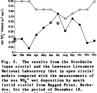
provided our network observations of precipitation with climatological con- texts. We used these climatological data to extrapolate from the limited measurements in our comparison of the

modeled with measured

non-sea-salt S04

=

There was also a question about how representative the aerosol concentra- tions were when compared with the model

outputs. The actual observations might

have underestimated the reality. The aerosol samplers were sector controlled

to minimize the influence of local

sources. At each AEROCE site when the

winds at tower height were blowing across the island, no aerosol samples were taken. This reduced sample collec-

tion times to less than 100%. At Barba-

dos the winds were out of sector less

than 10% of the time on average; however

at Mace Head and Bermuda, out-of-sector

winds were more frequent and the sector-

controlled measurements were biased.

Since tower-level winds at Mace Head

were not sampled when they came from the

east (crossing Ireland), an important

fraction of aerosol-laden air masses

from Europe could have been missed.

These exclusions of winds resulted in

aerosol signatures that were more repre-

sentative of aerosol concentrations over

the North Atlantic Ocean. Since the

models simulated all flow conditions, we

had to consider the aerosol observations

at Mace Head as biased concentrations

that underestimated the real conditions

86

Galloway et al.: Field-btodel Synthesis for Atmospheric S and N

3. THE CASE STUDIES

3.1. The Sulfate Comparison Case Study

This case study compared predictions from three models--the 0slo model liver-

sen, 1989], the Stockholm model [Langner

and Rodhe, 1990], and the LLNL model [Walton et al., 1988; Erickson et al.,

1991]--with data collected by the AEROCE and WATOX programs. First, we examined

the predict ions for the concentrations of sulfur dioxide and particulate

sulfate and the wet deposition of sulfur as given by the three models for Yanuary

and Yuly. Second, we compared the model

calculations with the actual measure-

ments of the S04

= concentrations in the

sites--Mace Head, Ireland; Bermuda;

Barbados; and Tenerife, Spain--and the

sulfate wet deposition from Barbados,

Bermuda, and Mace Head.

3.1.1. Comparisons among the three

models. We examined the model results

for Yanuary and Yuly. The predicted

distributions of particulate-sulfate

concentrations in the surface level air

are shown in Figure 2. There was a fun-

damental difference in the meteorologi- cal representation of these data. The

Stockholm and LLNL models (Figures 2a and 2b) represented the distribution of particulate sulfate for a typical (cli- matological) Yanuary weather situation, whereas the Oslo model (Figure 2c)

depicted the situation specifically for

Yanuary 1983.

The three models predicted quite similar sulfate-concentration patterns.

The maximum concentrations occurred over

continental areas with the low concen-

tration bands over the mid-Atlantic

Ocean. The maximum concentrations were

larger over Europe than over North Amer-

ica because of the larger fossil-fuel sulfur sources. The Oslo model predict- ed higher maximum concentrations over Europe and North America than did the

Stockholm and LLNL models. Over central

Europe, the position of the maximum air concentration corresponded to the maxi-

mum emission area for the Stockholm

model and the Oslo model but was dis-

placed toward the north for the LLNL

model. All three models also predicted

troughs of roughly 10 to 20 nmol m

-3

over the mid-Atlantic Ocean.

The climatological models (the

Stockholm and LLNL models) showed

smoother gradients than the Oslo model,

which, as we have stated, used the

actual meteorology for Yanuary 1983. Consequently, the Oslo model showed a

SW-NE tilt for the North American con-

tours that reflected the particular

weather situation of that time.

We compared the model calculations

for the surface air concentrations and

the wet deposition for three selected

areas: over North America, over the

60ø•

50ø•

40ø•

30ø•

Fig. 2. The predicted sulfate concen-

trations from (a) the Stockholm model at

250 m (nanomoles per cubic meter), (b)

the Lawrence Livermore National Labora-

tory model at the surface (nanomoles per cubic meter), and (c) the Oslo model at 40 m (micromoles per cubic meter) for Yanuary when all sources were