Dynamics of particle clouds related to open-water sediment disposal

Dynamics of Particle Clouds Related to

Open-Water Sediment Disposal

by

Gordon J. Ruggaber

Submitted to the Department of Civil and Environmental Engineering

in partial fulfillment of the requirements for the degree of

Doctor of Philosophy in Environmental Engineering

ggG

at the

MASSACHUSETTS INSTITUTE OF TECHNOLOGY

June 2000

@

Massachusetts Institute of Technology 2000. All rights reserved.

Author ...

Department of Civil and Environmental lin'gineering

May 1, 2000

C ertified by ...

E. Eric Adams

Senior Research Engineer

Thesis Supervisor

Accepted by ....

Daniele Veneziano

Chairman, Departmental Committee on Graduate Studies

MASSACHUSETTS INSTITUTE OF TECHNOLOGY

MAY

_{3 0 2000}

_ENG

Dynamics of Particle Clouds Related to Open-Water

Sediment Disposal

by

Gordon J. Ruggaber

Submitted to the Department of Civil and Environmental Engineering on May 1, 2000, in partial fulfillment of the

requirements for the degree of

Doctor of Philosophy in Environmental Engineering

Abstract

Open-water disposal and capping is a promising solution for disposing of the 14 to 28 million m3 _{of contaminated sediment dredged annually in the United States}

(National Research Council, 1997). Such practice raises concerns about the feasibility of accurately placing the material in a targeted area and the loss of material to the environment during disposal. To better predict the fate of these materials, the objective of this research was to gain new insight into the physical processes governing the mechanics of their convective descent.

Instantaneously released sediments form axisymmetric "clouds" resembling self-similar thermals. Current particle cloud models employ thermal theory and an in-tegral approach using constant entrainment (a), drag (CD), and added mass (k) coefficients. The aim of this study was to investigate how real sediment characteris-tics (particle size, water content, and initial momentum) affect cloud behavior (i.e., velocity, growth rate, and loss of particles) and time variations in a, CD, and k.

Flow visualization experiments were conducted using a glass-walled tank, special sediment release and capture (i.e., "trap") mechanisms, and various cohesive and non-cohesive particles. Particle sizes were scaled to real-world dimensions through the cloud number (Nc), defined as the ratio of the particle settling velocity to the characteristic cloud velocity. An "inverse" integral model was developed in which the conservation equations were solved for a and k using measured velocity and radius data. Based on the "inverse" model results, particle cloud experiments were simulated with an integral model using constant and time-varying a and k.

The non-cohesive sediments evolved rapidly into "thermals" with asymptotic de-celeration and large growth rates (a = 0.2 - 0.3). The particles eventually organized into "circulating thermals," with linear growth rates obeying buoyant vortex ring theory. In this phase, large particles (Nc > 10-) produced laminar-like vortex rings with small a (0.1 - 0.2). Compared to the cohesive sediments, which exhibited a wide range of growth rates, changes in water content and initial momentum of the

non-cohesive particles produced 10 - 20 % variations in a.

behind the cloud, which contained as much as 30 % of the original mass depending on the release conditions. Much of the "stem" material either re-entrained into the cloud later in descent or reached the bottom shortly after it. Material not incorporated into the "stem," which may be advected by ambient currents, was found to be only a small fraction (< 1 %) of the original mass.

Inverse integral model results suggest that CD and k are close to zero within the "thermal" phase. In the "circulating thermal" phase, the reduction in a caused by large particles (Nc > 10-4) increased k to a value similar to that of a solid sphere. In-tegral model results confirm the suitability of using constant coefficients for modeling particle clouds with Nc less than 10-. When Nc is greater than 10-4, time-varying a and k are required to properly simulate cloud behavior in the "circulating thermal" phase.

Thesis Supervisor: E. Eric Adams Title: Senior Research Engineer

Acknowledgments

I would like to acknowledge the MIT Sea Grant College Program and the New England Division of the U.S. Army Corps of Engineers for sponsoring this research.

I would like to thank my thesis advisor, Dr. E. Eric Adams, for his helpful advice and direction provided over the course of this work. I wish to also show my sincere appreciation to my thesis committee members, Professor Ole S. Madsen, Professor Kelin Whipple, and Dr. Thomas Fredette, for their time, effort, and thoughtful input. I would like to recognize Scott Socolofsky for his help in constructing the ex-perimental facilities, programming the data acquisition software, and assisting with experiments. Special credit must be given to Elizabeth Bruce and Christopher Resto for their contributions to this work. Their many hours of assistance with experiments and data analysis are greatly appreciated. I wish to also thank Paul Fricker for his friendship and help with experiments as well as Ling Tang and Sanjay Pahuja for their friendship and moral support.

Special thanks go to Sheila Frankel for her many efforts in making Parsons Lab a more enjoyable place work.

I wish express my gratitude to my parents, Rudolf and Joan, and parents-in-law, Ben and Connie Sheffy, for all of their love and support during this endeavor.

Most of all, I am forever grateful to my wife, Alese, and children, Ben and Chelsea, for their constant love, encouragement, and patience over the past four years. Without their many sacrifices, my Ph.D. would not have been possible.

Contents

1 Introduction

1.1 _{M otivation . . . .} 1.2 _{Qualitative Description of Convective Descent . . . .} 1.3 _{O bjectives . . . .}

2 Background

2.1 _{T herm als . . . .} 2.1.1 _{Theoretical Analysis of Thermal . . . .} 2.1.2 _{Laboratory Studies of Thermals . . . .} 2.2 Buoyant Vortex Rings . . . . 2.2.1 _{Theoretical Analysis of Buoyant Vortex Rings . . . .} 2.2.2 _{Laboratory Studies of Buoyant Vortex Rings . . . .} 2.3 _{Particle Clouds . . . .} 2.3.1 _{Scaling Analysis of Particle Clouds . . . .} 2.3.2 _{Laboratory and Numerical Modeling Studies of Particle Cloud} 2.3.3 _{Field Studies of Particle Clouds . . . .}

3 Experimental Methods

3.1 _{Particle Types . . . .} 3.2 _{Sediment Release and Capture Mechanisms . . . .} 3.3 Flow Visualization . . . . 3.4 Image Processing . . . . 3.5 Experimental Procedure . . . . 13 13 15 19 21 21 21 26 27 27 31 31 32 36 41 45 45 47 48 54 60

4 Particle Cloud Experiments 61

4.1 A pproach . . . . 62

4.2 Cloud Growth Analysis . . . . 64

4.2.1 "Thermal" Phase . . . . 64

4.2.2 "Circulating Thermal" Phase . . . . 77

4.3 Velocity Analysis . . . . 81

4.4 Circulation Analysis . . . . 87

4.5 Discussion and Summary . . . . 92

5 Sediment Trap Experiments 97 5.1 Suspended Particles . . . . 97

5.1.1 Quantification of "Stem" Particles . . . . 97

5.1.2 Mass Distribution of Particles in "Stem" . . . . 102

5.1.3 Mass of Particles Excluded from "Stem" . . . . 111

5.2 Settled Particles . . . . 112

5.3 Settled Particles with Excess Water . . . . 113

5.4 Discussion and Summary . . . . 115

6 Integral Model Analysis 117 6.1 Model Development . . . . 118

6.2 Sensitivity Analysis . . . . 119

6.3 Inverse Modeling Results . . . . 122

6.3.1 Determination of Drag Coefficient . . . . 123

6.3.2 Determination of Added Mass Coefficient . . . . 129

6.4 Forward Model Analysis . . . . . . . . . . . 132

6.4.1 Model Simulations Using Constant Coefficients . . . . 132

6.4.2 Model Simulations Using Time-Varying Coefficients . . . . 139

6.5 Real-World Scaling - Case Study Simulations . . . . 150

7 Boston Blue Clay Experiments 155 7.1 A pproach . . . 155 7.2 Cloud Growth and Velocity Results . . . . 157 7.3 Conclusions . . . . 163

8 Conclusions and Recommendations for Future Work 167 8.1 Conclusions . . . . 167 8.2 Recommendations for Future Work . . . 170

A Experiment Cross-Reference Tables 173

B Selected Images for Group I, II, and III Experiments 175

C Radius and Center of Mass Profiles for Group I, II, and III

Experi-ments 189

D Entrainment Coefficient and Velocity Statistics 203 D.1 Entrainment Coefficient and Velocity Statistics - Experimental Groups

1, 11, and III. . . . 204 D.2 Example Radius and Velocity Profiles With Standard Deviations . . . 205 D.3 Effect of 100 % and 150 % Cropping Criteria on Entrainment Coefficients210

E Results for 0.556 mm Glass Bead Experiments 211 E.1 Selected Images for "Wet" Experiments . . . . 213 E.2 Equivalent Radius and Velocity Profiles . . . . 218 E.3 Entrainment Coefficients and Velocity Data . . . . 223

List of Figures

1-1 _{Idealized particle cloud phases (after Brandsma and Divoky, 1976). 16} 1-2 Idealized particle cloud convective descent phases. . . . . 18 2-1 Particle size correlation between 40 g laboratory sample and real-world

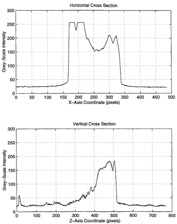
barge sizes based on cloud number scaling. . . . . 34 3-1 Sediment release mechanism (scale: base is 15.2 cm x 15.2 cm). . . . 49 3-2 Sediment trap mechanism (scale: frame is 92 cm x 92 cm). . . . . 50 3-3 Flow visualization tank (after Socolofsky, 2000). . . . . 51 3-4 Image acquisition system (after Bruce, 1998). . . . . 53 3-5 _{Grey-scale intensity profiles for representative horizontal and vertical}

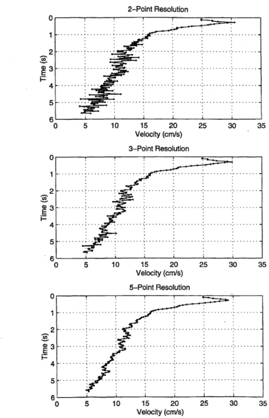
cross sections of a 0.264 mm particle cloud image. . . . . 55 3-6 _{Representative velocity profiles for a 0.264 mm particle cloud based on}

2-point, 3-point, and 5-point resolutions. . . . . 59

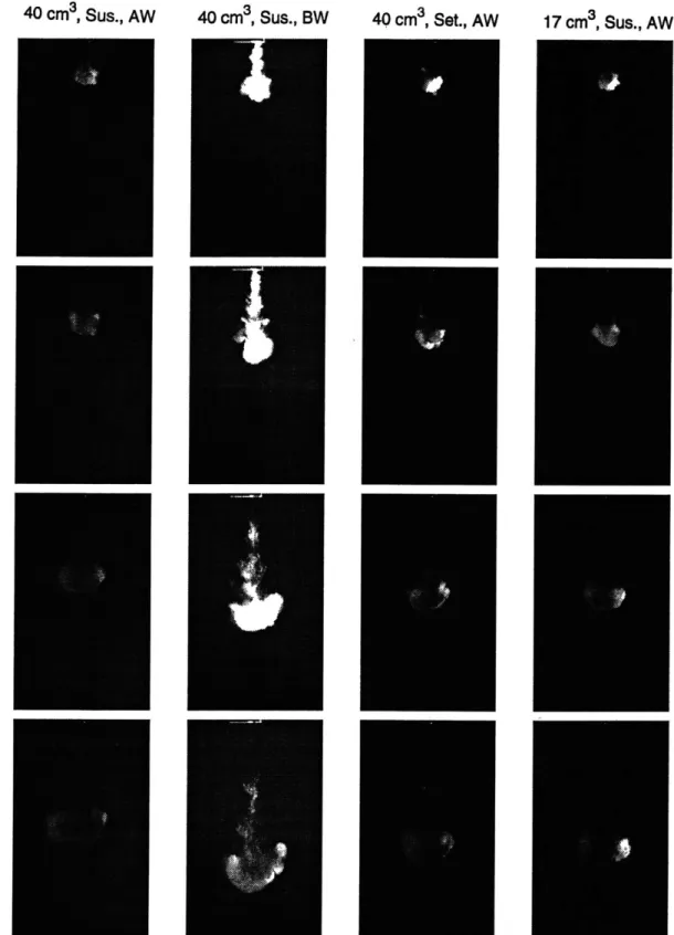
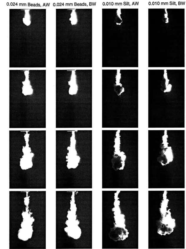
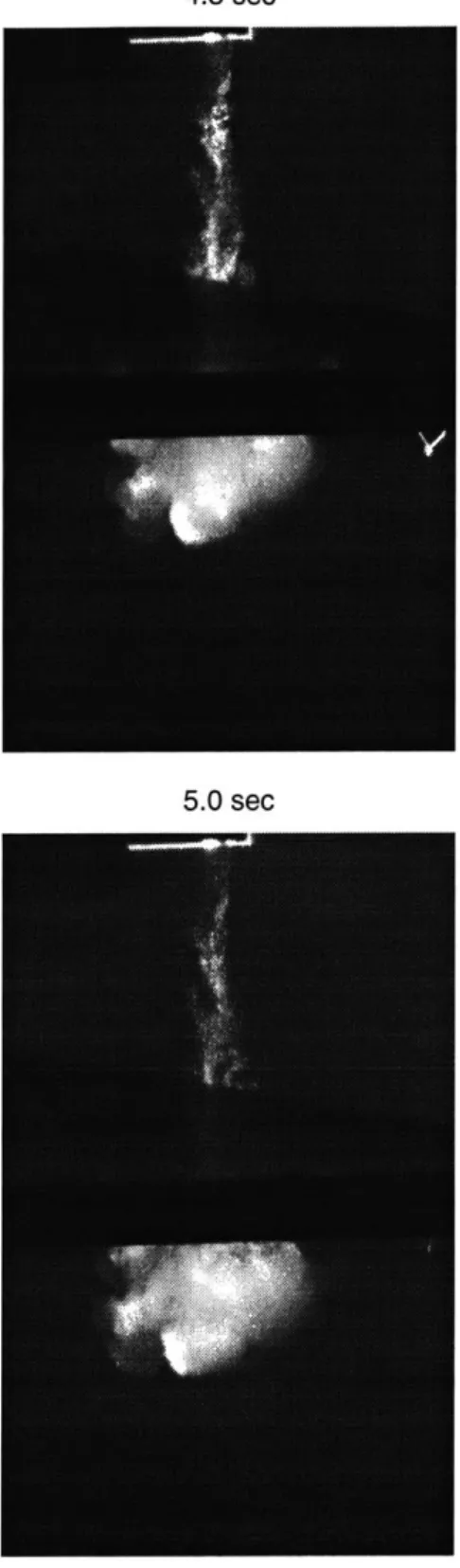
4-1 Selected cloud images for first 0.6 s of descent - Group I "Wet" exper-iments. Actual size of frames is approx. 64 cm x 87 cm. . . . . 65 4-2 Selected cloud images at 1 s, 2 s, 3 s, and 4 s - Group I experiments.

Actual size of frames is approx. 64 cm x 87 cm. . . . . 66 4-3 selected cloud images at 1 s, 2 s, 4 s, and 6 s - Group II experiments.

Actual size of "AW" frames is approx. 88 cm x 116 cm. Actual size of "BW" frames is approx. 69 cm x 91 cm. . . . . 67 4-4 Selected cloud images at 1 s, 2 s, 4 s, and 6 s - Group III experiments.

4-5 Equivalent radius versus center of mass position with fitted linear re-gression lines - Group I experiments. Open circles denote pre-release

radius and center of mass position. . . . . 74

4-6 Equivalent radius versus center of mass position with fitted linear re-gression lines - Group II experiments. Open circles denote pre-release radius and center of mass position. . . . . 75

4-7 Equivalent radius versus center of mass position with fitted linear re-gression lines -Group III experiments. Open circles denote pre-release radius and center of mass position. . . . . 76

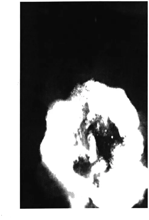
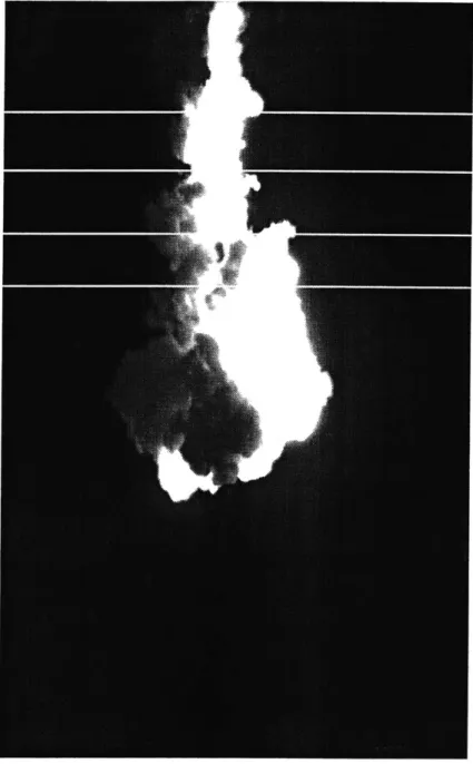
4-8 Top view of cloud at 4 s - 4.45 cm Cyl. "Wet" experiment. . . . . 78

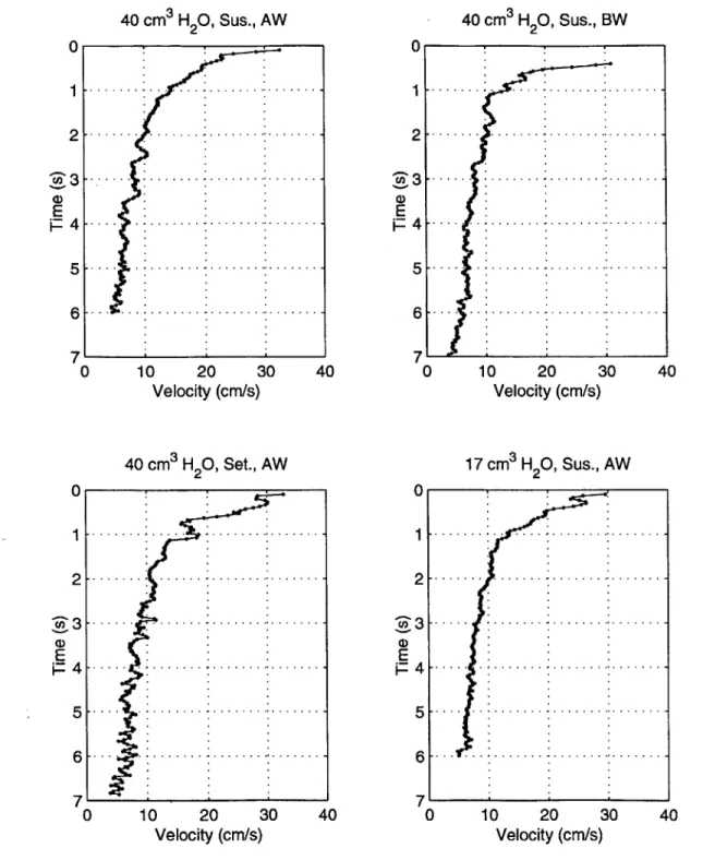
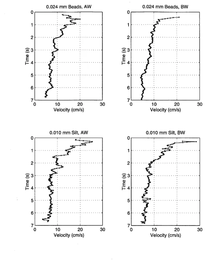
4-9 Center of mass velocity versus time - Group I experiments. . . . . 82

4-10 Center of mass velocity versus time - Group II experiments. . . . . . 83

4-11 Center of mass velocity versus time - Group III experiments. . . . . . 84

4-12 Log-log plots of center of mass velocity versus time - experimental Groups 1, 11, and III. Straight lines are fitted linear regression lines w ith - 0.5 slope. . . . . 86

4-13 Circulation coefficients and circulation versus time - Group I "Wet" Experiments. Middle K plots based on time-varying c; lower K plots based on c 0.46... .. . .. . . .. . . . . 89

4-14 Predicted vortex ring core and hole diameters superimposed on selected cloud im ages at 4 s. . . . . 93

5-1 Before and after images of 0.264 mm particle cloud descending through sedim ent trap. . . . . 99

5-2 Sediment trap locations for determining "stem" mass distribution for 0.010 mm "BW" silt experiment. . . . . 103 5-3 Time-variation of particle mass remaining in release cylinder for 0.010

mm silt and 0.264 mm bead "BW" experiments. Open circles denote measured data. Solid lines show fitted exponentially decreasing functions. 105

5-4 Selected images from 0.264 mm bead "BW" experiment showing shal-low and deep sediment trap locations. . . . . 107 5-5 Selected images showing emergence of secondary plume in sediment

trap experim ents. . . . . 109 5-6 Selected images from 0.010 mm silt "BW" experiment showing

approx-imate leading edge locations of secondary plumes. . . . . 110

6-1 Forward model sensitivity analysis results. In left column plots, CD, k = 0.25 and a = 0.1 and a = 0.5 denoted by solid and dashed lines, re-spectively. In right column plots, a = 0.25 and CD, k = 0.01 and

CD, k - 0.5 denoted by solid and dashed lines, respectively. . . . . 121 6-2 Examples of smooth curves fitted to measured velocity and radius data

using t-05 functions and 6th-order polynomials, respectively. . . . . . 124 6-3 Inverse model results for drag coefficient (CD) for 0.264 mm bead

ex-periments. Results using k = 0.01 and k = 0.5 denoted by thick and thin lines, respectively. . . . . 125 6-4 Inverse model results for drag coefficient (CD) for 0.024 mm bead and

0.010 mm silt experiments. Results using k = 0.01 and k = 0.5 denoted by thick and thin lines, respectively. . . . . 126 6-5 Comparison of smooth curves fitted to measured velocity and radius

data for 0.024 mm bead "AW" and "BW" experiments. . . . 128 6-6 Inverse model results for added mass coefficient (k) for 0.264 mm bead

experiments. Results using CD = 0.01 and CD = 0.5 denoted by thick and thin lines, respectively. . . . . 130 6-7 Inverse model results for added mass coefficient (k) for 0.024 mm bead

and 0.010 mm silt experiments. Results using CD = 0.01 and CD = 0.5 denoted by thick and thin lines, respectively. . . . . 131 6-8 Forward model results using constant coefficients for 0.264 mm bead

6-9 Forward model results using constant coefficients for 0.264 mm bead "Suspended" experiments. Simulation results denoted by thin lines. . 136 6-10 Forward model results using constant coefficients for 0.024 mm bead

"AW" and "BW" experiments. Simulation results denoted by thin lines. 137 6-11 Forward model results using constant coefficients for 0.010 mm silt

"AW" and "BW" experiments. Simulation results denoted by thin lines. 138 6-12 Forward model results using constant coefficients with mean a for 0.264

mm bead "Settled" experiments. Simulation results denoted by thin lines. ... ... .... ... .. .140 6-13 Hyperbolic tangent functions for a for "Settled" and "Suspended" bead

experim ents. . . . . 142 6-14 Forward model results using time-varying a and constant k for 0.264

mm bead "Settled" experiments. Simulation results denoted by thin lin es. . . . . 143 6-15 Inverse model results for added mass coefficient (k) using tanh function

for a... . . . ... 145 6-16 Hyperbolic tangent functions for k for glass bead experiments. . . . . 146 6-17 Forward model results using time-varying a and k for 0.264 mm bead

"Settled" experiments. Simulation results denoted by thin lines. . . . 147 6-18 Forward model results using time-varying a and k for 0.264 mm bead

"Suspended" experiments. Simulation results denoted by thin lines. . 148 6-19 Forward model results using time-varying a and k for 0.024 mm bead

"AW" and "BW" experiments. Simulation results denoted by thin lines. 149 6-20 Real-world model simulation results using constant and time-varying

coefficients for 100ma, 1, 000m3_{, 5, 000m}3 _{barge volumes. Model results}

for constant and time-varying coefficients (a and k) denoted by thick and thin lines, respectively . . . . 152

7-1 Selected cloud images at 0.5 s, 1 s, 2 s, and 3 s - Boston Blue Clay experim ents. . . . . 158

7-2 Maximum radius versus leading edge position with fitted linear regres-sion lines - Boston Blue Clay experiments. . . . 160 7-3 Effect of moisture content on cloud velocity and entrainment coefficient

- harbor silt experiments (after Bowers and Goldenblatt, 1978). . . . 161

List of Tables

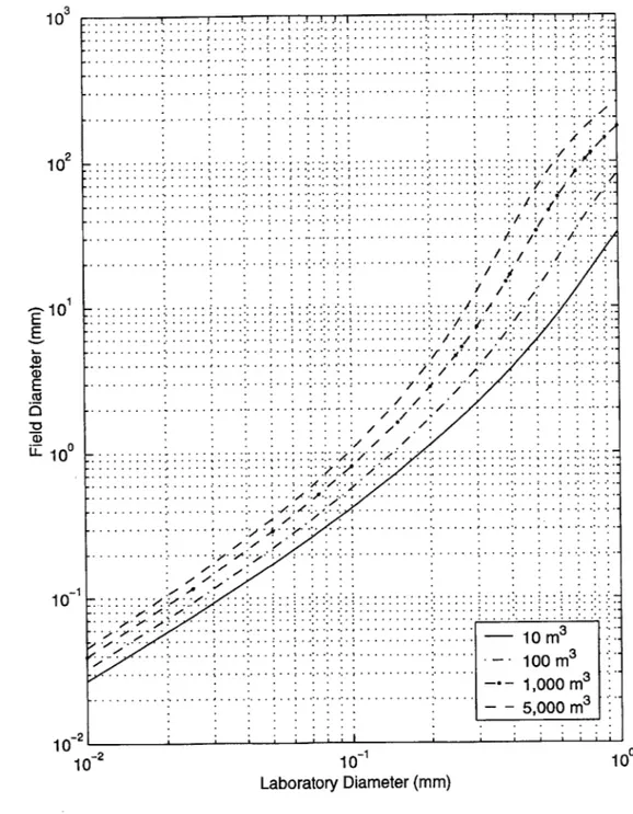
2.1 Nc scaling of particle cloud grain sizes between 27 cm3 _laboratory

volume and barge volumes of 10, 100, 1,000, and 5,000 m3_{. . . . 33}

3.1 Particle specifications for non-cohesive particles. . . . . 46

4.1 Initial condition variables - experimental Groups 1, 11, and III. ... 62

4.2 Release condition matrix - experimental Groups 1, 11, and III. .... 63

4.3 Release condition matrix - experimental Groups IV and V. . . . . 64

4.4 Initial cloud conditions - experimental Groups 1, 11, and III. . . . . . 69

4.5 Cloud growth parameters - experimental Groups 1, 11, and III. Time tc and depth ze denote the time and depth associated with the transition to "circulating thermal." . . . . 72

4.6 Entrainment coefficient values - experimental Groups IV and V. . . . 73

4.7 Velocity parameters - experimental Groups 1, 11, and III. . . . . 85

4.8 Normalized velocity comparison. . . . . 87

4.9 Circulation parameters - experimental Groups 1, 11, and III. . . . . . 90

4.10 Predicted geometric parameters for circulating thermals. . . . . 92

4.11 Entrainment coefficient comparison based on N . . . . . 95

5.1 Sediment trap results - suspended particle experiments. Trap depth denotes elevation of sediment trap. Closure time denotes time shade was drawn after release of particles. Percentages denote mass of "stem" particles retained on shade expressed as the percent of original mass. 100

5.2 Mass distribution in "stem" - 0.010 mm silt "BW" experiment. Per-cent values denote the amount of mass contained within the depth interval relative to the total mass in "stem." . . . . 104 5.3 Comparison of cloud center of mass velocity and secondary plume

lead-ing edge velocity for 0.010 mm silt and 0.264 mm bead "BW" experi-ments. Units for all velocities are _S.. . . . . 108 5.4 Sediment trap results - settled particle experiments. Trap depth

de-notes elevation of sediment trap. Closure time dede-notes time shade was drawn after release of particles. Percentages denote mass of "stem" particles retained on shade expressed as the percent of original mass. 112 5.5 Sediment trap results using silt tracer - settled particles/excess water

experiments. The % of total mass denotes the amount of captured silt relative to the total added silt. The % of supernatant denotes the amount of captured silt relative to the silt contained in the overlying water. . .. ... ... . . . ... . 114

6.1 Forward model parameters - constant coefficients. . . . . 133 6.2 Forward model parameters - time-varying coefficients. . . . . 141 6.3 Model parameters and initial conditions -shallow-water simulations. . 151

7.1 Entrainment coefficient results - Boston Blue Clay experimental results and interpolated values based on harbor silt experiments (from Bowers and Goldenblatt, 1978). . . . . 162

Chapter 1

Introduction

In this chapter, the real-world problems motivating this work are described. The scope of this investigation, as related to the ultimate fate of sediments discharged to open waters is discussed next, followed by an outline of objectives for this work.

1.1

Motivation

An estimated 14 to 28 million m3 _{of contaminated sedimentary material is dredged}

annually in the United States, which represents approximately 5 to 10 % of all sed-iments dredged in the U.S. (National Research Council, 1997). A lack of low-cost upland disposal alternatives has made open-water disposal followed by placement of capping materials (e.g., sand) an attractive solution. Such practice raises not only water quality concerns associated with the potential loss of contaminated material to the water column during disposal, but also engineering challenges related to the ability of barges or scows to accurately place dredged and capping materials within a targeted area.

The Boston Harbor Navigation Improvement Project (BHNIP) provides a timely example of the technological problems posed by a dredging disposal/capping project. The project, which involves dredging portions of Boston Harbor to accommodate newer and larger ocean vessels, is expected to ultimately generate about 1.0 million

m3

of contaminated silt, 2.7 million m3

and 0.1 million m3 _{of rock (Massport and USACE, 1995). The contaminated silt is}

being disposed of in excavated in-channel disposal cells (15-20 m deep) and covered with a 1 m layer of clean sand, while the parent material is being disposed of at the Massachusetts Bay Disposal Site (approximately 90 m deep). Implementation of a test cell in the summer of 1997 resulted in unanswered questions concerning the amount of lateral spreading (surging) that occurred following disposal of the silt material, as well as the amount of mixing that took place during placement of the coarser sand cap on top of the softer sediments (SAIC, 1997).

Clearly, successful implementation of sediment disposal and capping technologies, whether in shallow depths, such as Boston Harbor, or in deeper and more ecologically sensitive areas, requires an understanding of, and the ability to predict, the short-term mechanics of these materials in the environment (i.e., velocity, growth rate, and loss of particles to the environment). As discussed in Chapter 2, a limited number of studies have been performed to investigate the behavior of particle clouds as related to the disposal of dredged material. Thescopes of these studies were rather limited in that only gross comparisons were made between the motion of the particle clouds and that of classical "thermals." No detailed studies have been performed to investigate the influence of real sediment characteristics and release conditions (e.g., in-vessel set-tling, water content, initial momentum) on the behavior of released sediments. Field measurements suggest that the amount of material lost to the ambient environment during disposal to be in the range of 1 to 5 % of the original mass. However, to date, no studies have been conducted to investigate the physical mechanisms responsible for this loss and how such mechanisms are affected by initial sediment conditions. Hence, the aim of this research is to gain new insight intohow initial sediment characteristics and release conditions affect the physical processes governing the short-term fate of dredged and capping materials discharged into open waters.

The short-term behavior of materials discharged into open waters has been con-ceptualized into the following three phases (Clark et al., 1971; Koh and Chang, 1973) as shown in Figure 1.1:

trans-ported downward by its negative buoyancy (submerged weight).

" Dynamic Collapse: When the cloud impacts the bottom or reaches a level of neutral buoyancy, the cloud collapses and spreads horizontally.

" Passive diffusion: When dynamic spreading has ceased, cloud particles advect and diffuse through action of the ambient current.

The research discussed herein focuses on the first phase of particle clouds, convective descent.

1.2

Qualitative

Description of Convective Descent

It is most convenient to view the motion of suspended particles from a macroscopic point of view in which the particle cloud is assumed to act as a distributed source of negative buoyancy released suddenly (i.e., instantaneously) to its surroundings. In this respect, the cloud of particles is viewed as a continuous, single-phase density field, no different than a source of heavy fluid with the same average density. In the meteorological and fluid mechanics literature, such a sudden release of buoyancy (either positive or negative with respect to the ambient fluid) has been given the name "thermal" (Scorer, 1958; Woodward, 1959) based on early studies of free convection in the atmosphere due to temperature differences (e.g., cumulus cloud formation). Herein, the term "thermal" will be used in the context of a heavy thermal, falling through a fluid of lower density.

The typical velocity profile of a particle cloud has been categorized into the fol-lowing three regimes (Rahimipour and Wilkinson, 1992; Noh and Fernando, 1993) as shown in Figure 1.2:

" Initial Acceleration Phase

" Self-Preserving or Thermal Phase

-..-tvj... CONVECTIVE DESCENT ENCOUNTER NEUTRAL BUOYANCY DYNAMIC COLLAPSE IN WATER COLUMN LONG-TERM PASSIVE DIFFUSION DIFFUSIVE SPREADING GREATER THAN DYNAMIC SPREADING

Figure 1-1: Idealized particle cloud phases (after Brandsma and Divoky, 1976).

- -.- P, -1- - --

l-)z

Initial Acceleration Phase:

Upon release, the sediment/fluid mixture accelerates and expands rapidly, entrain-ing ambient fluid over all of its surface through the action of small, turbulent eddies produced by the hydrostatic instability associated with density differences and veloc-ity shear at the cloud boundary. It has been shown theoretically and experimentally (Escudier and Maxworthy, 1973; Baines and Hopfinger, 1984) that the duration of the initial acceleration phase is a function of the initial buoyancy, and that a thermal will typically reach the self-preserving phase after it has traveled a depth equivalent to 1 - _{3 initial cloud diameters. Similar durations have also been observed for particle} clouds (Nakatsuji et al., 1990; Li, 1997).

Self-Preserving Phase:

In this phase, thermals and particle clouds undergo an asymptotic deceleration caused by the rapid entrainment of less dense ambient fluid into the cloud. Since there is no representative length scale in this region, it is typically assumed that the thermal has reached a state of self-similarity in which all lengths are in proportion, and the mean velocity and buoyancy profiles across a horizontal section of the cloud are similar at all depths (Batchelor, 1954; Morton, Taylor, and Turner, 1956). Ini-tially, the distribution of buoyancy must resemble either a tophat or gaussian-type profile, with a maximum value in the center of the cloud. As the cloud grows, larger eddies are produced which induce flow of ambient fluid into the rear of the cloud. These large eddies are responsible for organizing the cloud into an axisymmetic, vor-tical structure similar to a vortex ring, or more accurately, a spherical vortex as described by Hill (1894). The buoyancy distribution in a vortex ring is bimodal, with the buoyancy concentrated in the rotating core. The spherical vortex is characterized by a downflow of fluid (and particles) through the center and upflow of fluid along the edges. As this structure matures, the induced internal circulation cause the cloud to flatten and evolve into the characteristic mushroom-shaped (upside-down) thermal.

E

Dispersive Phase

-Velocity

Dispersive Phase:

As the descending particle cloud decelerates and its velocity approaches the set-tling velocity of the individual particles, the circulation is insufficient to keep the particles in suspension. At this point, the particles settle out of the cloud leaving behind a neutrally buoyant fluid volume descending only with the inertia it possesses at that time. The settling particles descend as a particle "swarm" (Nakatsuji et al., 1990; Papantoniou et al., 1990; Biihler and Papantoniou, 1991) that continues to ex-pand (at a much slower rate) via weak inter-particle dispersive pressures (Rahimipour and Wilkinson, 1992).

1.3

Objectives

The goal of this research is to improve our understanding of the factors influencing the convective descent phase of particle clouds. The specific objectives of this work are to answer the following questions:

" Under the expected range of sediment disposal scenarios, do real sediments orga-nize into self-similar clouds that behave as dense "thermals" during convective descent?

" What roles do the initial conditions, namely particle size, water content, and initial momentum, play in determining cloud behavior within the initial accel-eration and self-preserving phases?

" What mechanisms are responsible for the loss of cloud particles and fluid to the environment during initial formation and convective descent?

" How accurately can the behavior of particle clouds be predicted using an integral-type model with constant entrainment, drag, and added mass coefficients?

* How do the entrainment, drag, and added mass coefficients vary in time and space during convective descent, and how are they affected by the initial con-ditions?

Chapter 2

Background

As noted in Chapter 1, during convective descent, particle clouds behave similarly to classical thermals and buoyant vortex rings, both of which have been the subject of several key studies, some dating back to the late 1950's and early 1960's. Thus, an understanding of the characteristics of these convective elements provides a basis on which to investigate the dynamics of particle clouds. To this end, the results of early studies of thermals and vortex rings are discussed in the first two sections, followed

by a synopsis of more recent particle cloud investigations.

2.1

Thermals

In this section, the theoretical analysis of thermals will be discussed first followed by a review of some key laboratory studies. In this section, the terms "thermal" and "cloud" are used interchangeably.

2.1.1

Theoretical Analysis of Thermal

In the analysis of thermals, it is convenient to use an integral approach in which the thermal is treated as a moving, expanding control volume (e.g., sphere or hemisphere) for which the following conservation equations apply in a uniform density environ-ment (Koh and Chang, 1973):

Conservation of Mass: d (21 d

(pr)

where: r is the thermal radius; V is the cloud volume; p and pa are the densities of the cloud and ambient fluid, respectively; k and CD are the added mass and drag

coefficients, respectively; and g is the gravitational constant. Equation 2.3 is based on the assumption that no buoyancy is lost to the wake of the thermal. Equation 2.1 is based on the classic entrainment assumption that the mean entrainment velocity is proportional to the mean center of mass velocity (w) through the entrainment coefficient (a). Hence, the mean flow rate of ambient fluid into the cloud is equal to the entrainment velocity multiplied by the surface area of the cloud. By assuming

p a Pa, setting w = L, and using the chain rule of differentiation, it can be shown

that:

r = az (2.4)

where z is the center of mass position.

Thus, use of the continuity equation and entrainment assumption results in a linear relationship between r and z, in which case a can be regarded as both a spreading angle (i.e., 1 = tana) and an entrainment coefficient. The assumption

that p pa represents a type of Boussinesq approximation, where it is assumed that

retained only in the buoyancy term.

Baines and Hopfinger (1984) used dimensional arguments to show that when the Boussinesq approximation is not made, Equation 2.4 should be modified as follows:

r = a "3 z (2.5)

The authors noted that the functional dependency of r on the ratio P- made physical sense since the static instability at the cloud surface producing the entrain-ing eddies is known to depend on the density difference between the thermal and the ambient fluid. Baines and Hopfinger also demonstrated both theoretically and experimentally that the entrainment rate for thermals is so large that the Boussinesq approximation is reached after the thermal descends about two initial diameters.

The three conservation equations contain three unknown variables (r, w, and p) and three unknown coefficients (a, k, and CD), which are largely empirical in nature and need to be determined by experiment. The equations do not permit an analytical solution without the use of simplifying assumptions, since elimination of two of the variables results in a second-order nonlinear differential equation in terms of the remaining variable.

If constant pressure and inviscid conditions are assumed (i.e., rate of work done by pressure and viscous shear forces is negligible), dimensional analysis can be used to derive the following similarity solutions for the motion of an axisymmetric thermal in a uniform density environment originating from a point source (Turner, 1973):

r = az

w =

(B

Ba r

g' = (B)z-3f2 ()

where: r is a position vector relative to the axis of symmetry; g' is the modified

respectively. Using an integral approach and neglecting the velocity and buoyancy distributions within the interior of the cloud, the following time dependencies for r

and w can be deduced using w = d (Turner, 1973):

1

Pa

w

(B- t (2.7)

Pa

Using some simplifying assumptions, Wang (1971) and Escudier and Maxworthy (1973) derived asymptotic solutions to the three conservation equations that are ap-plicable to very short (i.e., early in the initial acceleration phase) and long times (i.e., well into deceleration phase). The authors nondimensionalized the equations by in-troducing the characteristic (i.e., initial) length scale, r0, and buoyancy, F, (PoP-P),_Pa

and defining the following dimensionless variables:

r ~ agF' - a

r =- ; t= t - w = l w (2.8)

To (ro roFog

Assuming that the drag forces are small and can be neglected, and that there is no loss of fluid (buoyancy) to the thermal's wake, Escudier and Maxworthy (1973) derived the following asymptotic solutions for a spherical thermal:

Short times, (f - 1) < 1: 2(1 + k) - Fo ' + k - Fo (2.9) Long times, f

>

In dimensional form, Equation 2.10 yields the following:

3aB t 3B - 1_(2.11)

r = -~ w = (211

47rpa/ (2(1 + k)) ' 47pa I(2a)4( +k)(

Equation 2.11 is similar in form to Equation 2.7 except for the constant coef-ficients, functionality in a, and inclusion of the added mass coefficient (k). These differences are the result of the inclusion of k in the momentum equation by Escudier and Maxworthy (1973) as well as their choice of nondimensional parameters and their inclusion of a.

Morton et al. (1956) provided the first theoretical development of the behavior of thermals in a stably stratified environment in which they used, in addition to the mass and momentum conservation equations, the following conservation of buoyancy principle:

dj J(P - pa(0))dV = 4r 2aw(pa - pa(0)) (2.12)

where pa(0) is the reference density of the ambient fluid taken at z = 0. In words, Equation 2.12 states that the time rate of change in buoyancy, integrated over the entire volume of the thermal, is equal to the inflow of buoyancy integrated over the surface area of the cloud. By substituting the mass and momentum conservation equations into Equation 2.12, neglecting the added mass and drag force, and using the Boussinesq approximation, Morton et al. (1956) expressed the conservation of buoyancy in terms of the Brunt-Viisils frequency (N) as follows:

-- (r3g (PPa)

)

where N2 _{= q P.a Morton et al. (1956) nondimensionalized the conservation}

pa(o) dz*

equations and normalized the time scale by N (i.e., ti = Nt; 0 < ti 27), which resulted in the following solutions for w and maximum, or "trap," depth (zmax):

3 Bo 4 (1~-i - NsW (Pa) zm3 ~B) a-1 Ni _(2.14) Pa where sinti W - Z ,8 Z-4(1-costi) , for ti <7r (1 - costi) I sinti i

W=-aZ=8-2 4(3 +cos ti)' ,

f

Thus, for a negatively buoyant thermal, zmax is proportional to B0 4 and inversely proportional to N2, since the falling cloud entrains positively buoyant fluid from the upper layers thereby increasing its buoyancy. The cloud eventually reaches a point where its velocity reverses sign and begins to oscillate around the level of neutral buoyancy at the frequency, N. The oscillation results from the fact that the cloud still possesses some momentum when it first reaches the point of neutral buoyancy, causing it to overshoot this level. At this point, its buoyancy becomes positive with respect to its surroundings causing it to rise and the oscillations to begin. Although not included in Equation 2.14, drag forces eventually dampen the oscillations, and the density stratification causes the cloud to collapse (i.e., enter dynamic collapse phase) and spread horizontally as the interior fluid seeks a hydrostatic equilibrium with the ambient fluid. By replacing the sine and cosine functions in W by their Taylor series expansions and neglecting higher order terms (i.e., sin ti ~ ti; cos ti ~ 1 -

}t

Equation 2.14 reduces to a form similar to that of Equation 2.11 when ti approaches zero.

2.1.2

Laboratory Studies of Thermals

Early experiments with thermals in the 1950's and 1960's were motivated by meteoro-logical phenomena (e.g.. cumulus clouds), whereas dredged material disposal concerns

provided the impetus for later experiments conducted during the past decade. Labo-ratory procedures in the early experiments involved releasing a dense fluid, usually a salt solution, into an illuminated, quiescent tank by manually inverting a hemispher-ical cup at the water surface. The descent of the thermal was then recorded on video tape from which velocity and entrainment estimates were made. In conjunction with these experiments, Equation 2.4 was used to determine a, and dimensional analysis was used to derive the following similarity solutions:

w = C(gFor)i (Scorer, 1957) (2.15)

2 -3B

z =cia- - t (Richards, 1961) (2.16)

Pa

where C and ci are constants.

Scorer (1957) reported values of a ranging from 0.20 to 0.34 with a mean of 0.25. Woodward reported an average value of 0.27 for a, whereas Richards (1961) reported a values between 0.13 and 0.53. These authors noted that the entrainment rate was quite sensitive to the initial release condition (i.e., the manner in which the cup was inverted), which was difficult to reproduce consistently, but that a remained roughly constant in a given experiment. Scorer (1957) calculated a mean value of 1.2 for C, which, not surprisingly, exhibited variability similar to that of a, since Turner (1964) showed that the two coefficients are related as follows: C2_{a(1 - a) = 1. In contrast,}

Richards found that ci = _{0.73 for nearly all of the thermals in his experiments.} Turner (1964) showed that ci is mainly a function of the shape of the thermal and the associated added mass coefficient, with only a small dependence on a.

2.2

Buoyant Vortex Rings

2.2.1

_{Theoretical Analysis of Buoyant Vortex Rings}

It is instructive to compare the motion of a thermal, which moves from rest under its own buoyancy, to that of a buoyant vortex ring, which, in addition to buoyancy,

is generated with initial momentum, or impulse (I), as well as circulation (K). The hydrodynamic impulse, defined as the total mechanical impulse of body forces re-quired to instantaneously generate a circulating volume (V) of fluid from rest, can be expressed as follows (Lamb, 1932):

1

I = -p x x wdV (2.17)

where x is a position vector, and w is the vorticity vector. For an axisymmetric vortex ring, which is a toroidal-shaped element with mean radius (r), and cross-sectional radius (a), Equation 2.17 becomes (in cylindrical coordinates):

p7r r2

wpdzdr (2.18)

A

where I is in the direction of motion (i.e., along z axis); A is the cross-sectional area of the ring (Tra 2); and wo is the azimuthal vorticity component. The circulation is related to w through the surface integral:

K = odzdr (2.19)

JA

Using Equations 2.18 and 2.19, Lamb (1932) defined the characteristic length scale, r 2 _{0 rPa K} K _Iresulting in I ~ 7rpaKr2. The conservation of momentum (impulse)

equation can now be expressed as follows:

dI dr2

-~7rpaK = BO (2.20)

dt dt

Recognizing that K = u ds, where u is the tangential velocity vector and ds is

an element of a contour enclosing A, leads to the following expression for the vertical

velocity of the ring (w):

W = C-- (2.21)

r

Turner (1957) integrated Equation 2.20 and used Equation 2.21 along with w dz_dt

to obtain:

B0

r =z (2.22)

c27r paK 2

The author related this equation to Equation 2.4 for a thermal by defining a new entrainment coefficient as follows:

BO

Bo

= " (2.23)

c2ir paK2

In deriving Equation 2.23, Turner assumed that the vorticity does not extend to the axis of the ring. This assumption allowed him to invoke Kelvin's circulation theorem along a circuit passing through the center of the ring and around the outside so that

dt 0, and thus K is constant. The assumption of constant circulation was based

on the heuristic argument that as the ring progresses, its diameter increases faster than the rate at which entrained fluid can spread from turbulent diffusion (Turner, 1957). Through Equation 2.23, Turner argued that the buoyant vortex ring represents a broader category of convective elements in which the buoyant thermal is a special case.

The following expression for w can be obtained by integrating Equation 2.20 and using Equation 2.21:

m~ a- Ko2 t 2 (2.24)

Thus, for a given initial KO, an increase in buoyancy produces a decrease in veloc-ity, which, at first, seems counter-intuitive since this conflicts with Equation 2.7. The physics can be explained by the fact that buoyancy serves to increase the expansion of the ring, which decreases the velocity since w ~ j. However, as Turner pointed out, B0 and K are not independent in a thermal since circulation is produced by the

K - vB and B, is constant in a uniform environment, the circulation in a thermal

must be constant in a uniform environment. Obviously, this condition does not hold for a thermal during the initial acceleration phase but only after it has reached the self-preserving phase. As Scorer (1957) noted, at this stage, the buoyancy profile within the thermal must change to a distribution that does not continue to produce circulation, at which point an equilibrium is reached in which the drag forces balance the portion of the buoyancy force producing the circulation.

The similarity solutions for the motion of a buoyant vortex ring in a stably strat-ified environment are very similar to the preceding analysis of buoyant vortex rings under isothermal conditions with the exception that the buoyancy is no longer con-stant but varies with the ambient density profile as follows:

dB

= -cN 2_{r w (2.25)}

dt

Not surprisingly, the above equation is identical in form to Equation 2.13 for a ther-mal. Hence, in addition to B, and K,, N must now be introduced into the similarity solution. Dimensional analysis based on these variables gives the following relation

for the maximum height (zmax):

Zmax =C

(

where ci is a constant. Expressions for w, r, and B may be obtained through

nor-malization and substitution into the governing equations in a manner similar to the

approach used by Morton et al. (1956) in their analysis of thermals. Based on his

analysis of I and K for a vortex ring, Turner (1960) showed that density stratification serves to decrease the circulation as follows:

dK - -sN2r2 _(2.27)

dt 2

2.2.2

Laboratory Studies of Buoyant Vortex Rings

Though a wealth of literature exists concerning research of vortex rings, few exper-imental studies have been performed on buoyant vortex rings. Turner (1957, 1960) conducted experiments in uniform density and stratified environments using light buoyant vortex rings with density differences ranging from 4 % to 18 %. Results from these experiments yielded values for c in Equation 2.21 ranging from 0.13 to 0.27, a mean value of 0.18 for a, and a value of 3 for s in Equation 2.27.

Maxworthy (1974) conducted flow visualization experiments with vortex rings (i.e., neutral buoyancy) produced by forcing a mass of fluid through a sharp-edged orifice by the motion of a piston. This apparatus produced turbulent vortex rings with a mean a value of 0.011. By taking the slope of nondimensionalized velocity versus depth data, Maxworthy (1974) also estimated the value of the drag coefficient (CD) to be in the range of 0.084 - 0.108 for an equivalent spherical volume.

In later experiments using more sophisticated flow visualization and laser-Doppler techniques, Maxworthy (1977) observed that compact, "well-organized" vortex rings grew at a much slower rate (mean c = 0.001) than those with "disorganized" cores with much larger entrainment coefficients (mean a = 0.015). The author hypothe-sized that the differences in entrainment rates were associated with the amount of turbulence within the ring and surrounding fluid.

2.3

Particle Clouds

In this section, a theoretical analysis of particle clouds is presented first, followed by a summary of laboratory and field studies conducted to date. The theoretical analysis includes a discussion of scaling arguments using the cloud number (Nc) and a brief summary of some theoretical and empirical relationships for particle cloud behavior in the dispersive (particle settling) phase.

2.3.1

Scaling Analysis of Particle Clouds

For a particle cloud, the initial buoyancy (B0) can be computed simply from the

submerged weight of the particles as follows:

BO = m(1 - "a )g (2.28)

Ps

where m is the total mass of particles in the cloud, and p, is the density of an individual particle.

For fully turbulent particle clouds for which viscous effects can be ignored, di-mensional analysis can be used to derive the following characteristic cloud velocity scale:

BO

wo = " (2.29)

Equation 2.29 can also be derived by equating the drag and buoyancy forces.

Rahimipour and Wilkinson (1992) defined the cloud number (Nc) as the ratio of

particle settling velocity (w.) to the characteristic cloud velocity (wo), which, using

Equation 2.29, simplifies to the following expression for non-cohesive particles:

Ne = wr Pa) 2 (2.30)

(B

Since Nc is proportional to the cloud radius, its magnitude continually increases as

the cloud descends and grows. Since w, is related to particle diameter (d,) and wo is

related to the total mass or volume of particles, the cloud number can be viewed as a

type of size ratio, relating the mean grain size of the individual particles to the overall size of the cloud. Thus, Nc can be used to scale a small volume of small-diameter

particles in the laboratory to a larger volume of large-diameter particles released

from a full-scale barge. This type of scaling analysis was performed to determine

how a 40 g sample of particles (Bo = 23, 520 g cm s-2, V = 27 cm3_{), used for most}

of the experiments in this study, scales to much larger volumes in the real world.

Table 2.1: Nc scaling of particle cloud grain sizes between 27 cm3 _{laboratory volume}

and barge volumes of 10, 100, 1,000, and 5,000 m3

.

different full-scale volumes (i.e., 10 m3

, 100 Mi3

, 1, 000 m 3, and 5, 000 m3) by matching

the cloud numbers corresponding to the 40 g laboratory sample containing particles ranging from 0.01 - 1.0 mm in diameter. Settling velocities were calculated from particle diameters and vice versa using the following empirical relationship developed by Dietrich (1982) for spherical particles:

w* = -3.76715 + 1.92944 log(D*) - 0.09815 log(D*)2 _(2.31)

0.00557 log(D*)3 _{+ 0.00056 log(D*)}4

where

, wS3 _, (s - 1)gd,3 (s - 1)gv 'v2

and s is the specific gravity of a sediment grain (e.g., s = P = 2.5 for glass beads). The results of the cloud number scaling analysis are plotted in Figure 2.1 and tabulated in Table 2.1. Since Dietrich developed Equation 2.31 using velocity data for particles sizes ranging from 0.01 mm to about 100 mm in diameter, the accuracy of the scaling analysis for particles above this size is uncertain.

As shown in Table 2.1, results of the Nc scaling analysis show that laboratory-sized sand and silt particles scale to real-world dimensions by factors of - and , respectively. Thus, use of large particle sizes in the lab (i.e., 0.5 - 1.0 mm) scales

Laboratory Real-World Diameter (mm) Diameter (mm) 10 m3 100 m3 _{1,000 m}3 _{5,000 m}3 0.01 0.027 0.033 0.040 0.045 0.05 0.172 0.221 0.290 0.353 0.10 0.418 0.572 0.807 1.05 0.50 5.97 13.0 33.3 64.8 1.00 33.0 83.3 165 258

13 10 1 0 - . - -. --. -- . . . . .. -. - .- - - --. - -... ... . ... ... . . . . - . - -. . .. 1. .- .. . . . . . -. . - - , . -- -" -" -. * . -1 0 2 ; ; ; ; ; ;. ; ; .i ... ,... : : :,/,i:

/

Figure 2-1: Particle size correlation between 40 g laboratory sample and real-world barge sizes based on cloud number scaling.

to extremely large particles in the field (i.e., gravels and cobbles). Particles of this size must therefore be used with caution in the laboratory when attempting to repro-duce the real-world dynamics of particles of similar size using Nc scaling. Strict Nc compliance, however, may not be required to reproduce the dynamics of clouds with very small Nc (i.e., cloud dynamics may be insensitive to Nc). The influence of Ne on cloud behavior is discussed in Chapter 4.

As one might expect, flow visualization studies using different sizes of sand and glass beads show that three-dimensional, axisymmetric clouds enter the dispersive (particle settling) phase when the cloud velocity approaches the settling velocity of the particles (i.e., Nc -+ 1) (Rahimipour and Wilkinson, 1998; Biihler and Papantoniou,

1991; Boothroyd, 1971).

Based on experiments with two-dimensional particle clouds (i.e., originating from a line source), Noh and Fernando (1993) observed that the depth (Zd) associated with

the cloud's transition to the dispersive phase obeyed the following relationship:

ZdWs

(2.32)

where

Q

The authors hypothesized that, in addition to Nc, the transition depth depended on particle inertia, turbulent intensity, and inter-particle spacing. They noted that the transition occurred when Nc was less than 1, possibly due to the increase in particle settling velocity resulting from particle interactions and the downward background fluid velocity of the cloud.

Biihler and Papantoniou (1991) studied the growth rate of the particle "swarm" that emerges when the cloud transitions from the "thermal" to dispersive phase. Upon integrating the momentum equation and solving for the velocity by invoking the similarity assumption (i.e., !i- - w), the authors derived the following expression

1

/Bz N

r ~ 2(2.33)

Paws2

Biihler and Papantoniou (1999) explained that the growth of the particle swarm is caused by shear induced entrainment and lateral displacement flow resulting from the wake behind each particle.

2.3.2

_{Laboratory and Numerical Modeling Studies of}

Parti-cle Clouds

Bowers and Goldenblatt (1978) released samples of silty clay sediments containing various amounts of water to determine the effect of moisture content on entrainment. As will be discussed in Chapter 7, their results indicate that for cohesive materials, the entrainment coefficient is quite sensitive to water concentration. The authors note that samples with low water content tended to drop as clumps with virtually no entrainment, whereas more dilute slurries behaved very much like negatively buoyant thermals.

Nakatsuji et al. (1990) performed flow visualization experiments using 75-300

cm3 volumes of 0.8 mm, 1.3 mm, and 5.0 mm diameter glass beads. The authors derived a nondimensional expression for cloud velocity using conservation of mass and momentum equations similar in form to Equations 2.1 and 2.2. Using a and k values selected by the authors, their theoretical thermal velocity failed to accurately match measured velocities in the acceleration phase, as well as the cloud's peak velocity, which exceeds the predicted value by 20 %. The distance traveled during the initial acceleration period was equal to approximately 2.5 initial cloud diameters. Under the assumptions of constant a (0.4), constant k (1.0), no drag, and Boussinesq conditions, the authors showed that the smaller beads (< 1.3 mm) behaved according to thermal theory in the deceleration phase, whereas clouds formed from the larger 5 mm beads descended at a relatively constant speed, close to the settling velocity of the beads

(Nc

Tamai and Muraoka (1991) analyzed two-dimensional (i.e., line) particle clouds in the laboratory using fine (0.15 mm) and coarse (3.4 mm) sand. Their results showed linear growth rates (no a values given) and a velocity versus time profile that loosely follows thermal theory (i.e., w ~'-1 t-) for a line thermal. No information was provided by the authors as to how the theoretical curve was fit to the experimental data.

Rahimipour and Wilkinson (1992) conducted flow visualization experiments on particle clouds using graded sand (d, = 0.15 - 0.35mm). They compared velocity and growth rate data to analytical curves generated for a miscible thermal with the same buoyancy. Similar to the study by Nakatsuji et al. (1990), the authors show that thermal theory somewhat captures the decaying trend of cloud velocity in the asymp-totic (deceleration) region, after the cloud has traveled about two diameters, but does not predict velocities very accurately in the initial acceleration phase. By vary-ing initial volumes and particle sizes, Rahimipour and Wilkinson (1992), developed the following relationship between the entrainment coefficient and cloud number:

a= 0.31(1 - 0.44Nc12 5_{) for Nc < 1.5 (2.34)}

The above equation shows that, for small cloud numbers (i.e., Nc < 0.3), the entrainment rate remains approximately constant (a = 0.31), but decreases rapidly once Nc exceeds unity. The authors did not explicitly comment on when they consider the clouds to be in the dispersive phase (based on Nc) but note that the clouds are in the dispersive phase when Nc = 1.5. Rahimipour and Wilkinson (1992) derived the following empirical expression for the radial growth rate in the dispersive phase:

1 B 2 1

r 1.5 f

f

Pa Ws

Luketina and Wilkinson (1994) released particle clouds with various initial Nc values into a linearly stratified environment and compared maximum and final pene-tration depths to those predicted by an integral model based on the three conservation equations. Their model predicted maximum and final penetration depths that were consistently lower than measured experimentally. Their results confirmed the