An earth image simulation and tracking system for the Mars Laser Communication Demonstration

An Earth Image Simulation and Tracking System for the Mars

Laser Communication Demonstration

by

Stephanie Karen Balster

Bachelor of Science, Electrical Science and Engineering

Submitted to the Department of Electrical Engineering and Computer Science

in partial fulfillment of the requirements for the degree of

Master of Engineering in Electrical Engineering and Computer Science

at

the

Institute of Technology

May 5, 2005

_JUL

182005

Copyright 2005 M.I.T.

L R

E

LIBRA RIES

The author hereby grants to M.I.T. permission to reproduce and

distribute publicly paper and electronic copies of this thesis

and to grant others the right to do so.

Author

Depart'ent of Electrical Engineering and Computer Science

May 4, 2005 Certified by .

Frederick K. Knight V-A Company Thesis Supervisor Certified by ___

!e M. Freeman

sis ervisor

Accepted by

Arthur C. Smith Chairman, Department Committee on Graduate Theses

This report is based on studies performed at Lincoln Laboratory, a center of research

operated by the Massachusetts Institute of Technology. This work was sponsored by the

National Aeronautics and Space Administration under Air Force Contract

FA8721-05-C-0002. Opinions, interpretations, conclusions, and recommendations are those of the

author and not necessarily endorsed by the United States Government.

An Earth Image Simulation and Tracking System for the

Mars Laser Communication Demonstration

by

Stephanie Karen Balster

Submitted to the Department of Electrical Engineering and Computer Science on May 5, 2005, in partial fulfillment of the

requirements for the degree of

Master of Engineering in Electrical Engineering and Computer Science

Abstract

In this thesis I created an Earth-image simulation and investigated Earth-tracking algorithms for the Mars Laser Communication Demonstration (MLCD). The MLCD mission will demonstrate the feasibility of high-data-rate laser communications be-tween a Mars orbiting satellite and an Earth ground station. One of the key challenges of the mission is the requirement to achieve 0.35-prad-accuracy pointing and tracking of the laser beam to maintain the 1-30 Mbps communication downlink from Mars to Earth. The sunlit Earth is a bright source and, for most of the mission, can be tracked to stabilize the telescope from disturbances between 0.02 to 2 Hz, while other stabilization systems will cover the rest of the frequency spectrum. Before testing can-didate Earth-tracking algorithms, simulated Earth image sequences were created to provide test data sets. While a plain centroiding algorithm, thresholded-centroiding algorithm, cross-spectrum phase correlation method, and optical flow algorithm were all tested under various Earth phase conditions and pixel resolutions to evaluate their performance on simulated test data, the thresholded-centroiding algorithm was even-tually chosen for its accuracy and low computational cost. The effect of short-term albedo variations on the performance of the thresholded-centroiding algorithm was shown to be limited by the Earth's rotation and too slow to change the Earth's surface enough to affect the centroid calculation between time frames. Differences between the geometric centroid and optical centroid were measured to be up to 10% of the Earth's diameter, or up to 2 focal plane array pixels during the mission at closest range. As such, the uncertainty area in which to search for the beacon at the ground receiving station is limited to a 2-pixel radius.

VI-A Company Thesis Supervisor: Frederick K. Knight Title: Senior Staff, M.I.T. Lincoln Laboratory

M.I.T. Thesis Supervisor: Dennis M. Freeman Title: Associate Professor

Acknowledgments

I would like to thank my supervisor, Fred Knight, for all his guidance and support in my work on this thesis. Thank you to Bill Ross, Gary Long, Farzana Khatri, Jamie Burnside, Larry Candell, and Chris Ferraiolo, who have all been of tremendous help during my time at Lincoln. Thank you also to Professors Dennis Freeman and Jeffrey Shapiro, my advisors during my time at MIT.

Thank you to my family for all their support throughout the years, Mom, Dad, Chris, Jen, and GJ. Thank you to all my friends from MIT and Milpitas who have been with me through the good times and the bad, and especially thank you to Mark.

Contents

1 Introduction

1.1 The Mars Laser Communication Demonstration (MLCD) . . . .

1.2 Flight Terminal Pointing and Tracking Architecture . . . . 1.3 Thesis Goals and Approach . . . . 1.4 T hesis O utline . . . .

2 Generating Simulated Earth-Image Sequences

2.1 Related Work . . . .

2.2 Phenomenology . . . . 2.2.1 Overview . . . . 2.2.2 From Earth to Camera Image . . . 2.2.3 Albedo Variations . . . . 2.2.4 O ptics . . . . 2.2.5 Signal Level . . . . 2.2.6 Line-of-Sight Jitter . . . . 2.2.7 Focal Plane Array . . . . 2.3 Limitations of the Simulation . . . . 2.3.1 Earth's Terminator . . . .

2.3.2 Albedo Variations in Time . . . . . 2.3.3 Angular Jitter . . . .

2.3.4 FPA Pixel Gain and Offset Non-Uniformity . . . . 13 13 16 17 19 21 22 24 24 26 29 31 33 34 37 40 40 40 42 42

3 Tracking Algorithms 43

3.1 Related W ork .. .... ... . .. . .. .. ... . 44

3.2 Description of the Algorithms . . . . 44

3.2.1 Centroid Tracking . . . . 45

3.2.2 FFT-Based Cross-Spectrum Phase Correlation . . . . 46

3.2.3 Optical Flow . . . . 47

3.3 Algorithm Performance . . . . 48

3.3.1 Testing Method: The 1 A/D Case . . . . 48

3.3.2 Changing the MLCD Pixel Resolution: 2 and 2.5 A/D Pixels . 51 4 Using the Earth as a Tracking Reference 59 4.1 Related W ork . . . . 60

4.2 Earth Albedo Variations Over Time . . . . 61

4.3 Difference Between Optical and Physical Centroid . . . . 62

List of Figures

2-1 Earth images and e-/sec generated by Farzana Khatri's simulation for the MLCD mission with 1 A/D pixels, a) day 170 b) day 510 . . . . . 22 2-2 Sample Clementine mission 1-um images of the Earth, taken from the

NASA Planetary Image Atlas [11] . . . . 23 2-3 Distance between MTO satellite and Earth throughout the mission . 25 2-4 SEP angle between the Sun, Earth, and MTO satellite throughout the

m ission . . . . 25 2-5 SPE angle between the Sun, MTO satellite, and Earth throughout the

m ission . . . . 25 2-6 Conceptual block diagram for the Earth image simulation . . . . 27 2-7 Implementation block diagram for the Earth image simulation . . . . 28 2-8 Simulated Earth image after each major processing block a) Modified

Khatri Orbital Dynamics block b) Albedo Mapping (with signal flux added) c) Optics Subsystem d) Focal Plane Array . . . . 30 2-9 The Optics Subsystem . . . . 31 2-10 Airy point spread function for point source centered at (0,0) a) 2D

point spread b) cross-section at y=0 . . . . 32 2-11 Closed-loop LOS jitter spectra provided by Jamie Burnside a) x-direction

b) y-direction . . . . 36 2-12 Sample LOS movements provided by Jamie Burnside in a) 1 s time

period b) 4.8 ms time period. Note that the jitter is defined in units of 1 A/D pixels . . . . 37

2-13 Sample camera frame image a) before smearing added b) after smearing added ... ... ... ... 38 2-14 Simulated Earth images a) Day 160 b) Day 200 c) Day 300 d) Day 479

e) Day 600 f) Day 808 . . . . 41 2-15 Clementine image showing the Earth's terminator [11] . . . . 42 3-1 Illustration of the effects of the background in shifting the Earth

cen-troid location towards the center of the image, resulting in incorrect shift estimations by a plain centroiding algorithm due to this back-ground bias . . . . 46 3-2 Base images at 1 A/D pixel resolution a) Day 200 b) Day 300 c) Day

479 d) D ay 808 . . . . 49 3-3 Base images at 2 A/D pixel resolution a) Day 200 b) Day 300 c) Day

479 d) D ay 808 . . . . 53 3-4 Base images at 2.5 A/D pixel resolution a) Day 200 b) Day 300 c) Day

479 d) D ay 808 . . . . 54 4-1 Number of pixels covering 0.0035% of the Earth's diameter versus

mis-sion time to indicate that albedo changes due to the Earth's rotation are a small fraction of a pixel in an FPA frame time . . . . 63 4-2 Difference between optical and geometric Earth centroids in

Clemen-tine im ages . . . . 64

4-3 Optics test bench setup to simulate Earth and beacon images . . . . 65 4-4 Clementine images used to simulate albedo variations on the Earth

"source" . . . . 66 4-5 Experimental difference between optical and geometric centroid, in 2

List of Tables

1.1 Data rates required for various science data products . . . . 13 1.2 Optical and RF system parameters . . . . 15

2.1 Summary of camera pointing and tracking systems' operating condi-tion s . . . . 27 2.2 Percent reflectance at 1.06 pm of various Earth surfaces. Source: [14] 29 2.3 Parameter values for the optics subsystem . . . . 33 2.4 Parameter values for the focal plane array . . . . 39

3.1 1 A/D pixel resolution algorithm error statistics for varying Earth phase: maximum radial 1-A/D-pixel error, average radial 1-A/D-pixel error, and % errors meeting the 0.089-radial-diffraction-limited-pixel accuracy requirement . . . . 50 3.2 2 A/D pixel resolution algorithm error statistics for varying Earth

phase: maximum radial 1-A/D-pixel error, average radial 1-A/D-pixel error, and % errors meeting the 0.089-radial-diffraction-limited-pixel accuracy requirement . . . . 55 3.3 2.5 A/D pixel resolution algorithm error statistics for varying Earth

phase: maximum radial 1-A/D-pixel error, average radial 1-A/D-pixel error, and % errors meeting the 0.089-radial-diffraction-limited-pixel

Chapter 1

Introduction

1.1

The Mars Laser Communication

Demonstra-tion (MLCD)

The desire to gather more sophisticated science data, such as multi-spectral imagery,

SAR imagery, and HDTV, during future space exploration missions to the outer

planets calls for increased communication data rate capabilities of 10-100 Mbps and

higher. Currently, we use the Deep Space Network, a network of antennas in

Califor-nia, Spain, and Australia, on the Earth receiving end. With such a system, we can

support between 100 kbps

-

1 Mbps Radio Frequency (RF) data rates from Mars, a

factor of at least 100 less than our desired capability [8]. Table 1.1 shows the data

rates required for various science data products [5].

A study carried out at Caltech's Jet Propulsion Laboratory (JPL) on current and

Space Science Data

Data Rate

Planetary Images

10-100 kbps

Multi-Spectral Imagery

100 kbps

-

1 Gbps

Synthetic Aperture Radar

100 kbps

-

100 Mbps

Video (MPEG-1 to Raw Studio Quality)

1-100 Mbps

HDTV 10 Mbps - 1 Gbps

expected future laser communication technology capabilities suggests that an optical communication system can achieve the data rates desired for deep space communica-tions [6, 2]. As part of the ongoing effort to develop the capability of high data rate deep space communications, MIT Lincoln Laboratory, JPL, and NASA are working on the Mars Laser Communication Demonstration (MLCD) project. For this project, a laser communication system will be added to one of NASA's currently funded pro-grams to launch a communication satellite, the Mars Telesat Orbiter (MTO), to Mars in 2009. During the course of the MTO mission, the MLCD project will demonstrate the capability of achieving 1-30 Mbps data rates from Mars using 1.06-jm-wavelength laser communications.

The gain in achievable data rates for optical communications systems over RF systems comes from a number of parameter values, including the transmitted signal power, the beam divergence given by the communication wavelength and transmitter diameter, the receiver area, and noise. The gain of the optical over the RF system data rates follows the theoretical dependency:

Optical data rate Popt (DRF Rp NRF

RF data rate PRF oPt 2 R2F 2

Dopt

where P is the transmitted power, A is the communication wavelength, D is the transmitter diameter, R is the diameter of the receiver telescope, and N is the noise term. For systems configured as in Table 1.2, where the noise term in the RF case is at the thermal limit and the noise term in the Optical case is higher than the thermal limit, the optical system would be capable of achieving data rates 30 times those of the RF system.

One of the key advantages of using a laser communication system over an RF system comes from the difference in beam divergence for each system, determined by

A/D. A Ka-band beam through a 2 m diameter aperture in an RF system would

spread out over fractions of a degree, whereas for a laser communication system a 1 pm beam through a 30 cm aperture only spreads on the order of microradians [9]. For a communication system from Mars, an RF beam could spread to several times

Parameter

Optical

Ka-band RF

Transmitted Power 5 W 100 W

Wavelength, A 1.06 Ium 1 cm

Transmitter Diameter 30.5 cm 2 m

Receiver Diameter 5 m 60 m

Noise 600 kT/bit 2 kT/bit

Expected max data rate 30 Mbps 1 Mbps Table 1.2: Optical and RF system parameters

the diameter of the Earth, whereas a laser beam would only cover a small portion of the Earth's surface. The narrow laser beam thus focuses an increased fraction of the total signal power on the Earth receiving station, leading to lower required transmitted signal power and thus a lower-power spacecraft system overall that is more conducive to deep space missions. The tradeoff with laser communications comes from the increased precision required to point such a narrowly focused beam.

For the MLCD mission, the laser beam will need to be pointed at the ground station with a precision of within 10% of the laser beamwidth, whereas the orbital dynamics of the satellite, Mars, and Earth, jitter in the spacecraft, and noise in the optical system itself, will cause disturbances that are hundreds of times larger and over a wide range of frequencies. To aid in the pointing and tracking, an uplink beacon signal could be pointed from the ground station to the spacecraft to provide a reference to the spacecraft of where to point the transmitted downlink beam. Unfortunately, the power required to generate a beacon signal suitable for tracking fast enough to maintain the high data rate downlink is prohibitive, on the order of kilowatts. For the MLCD mission, a new scheme for pointing and tracking must be developed to meet this challenge.

1.2

Flight Terminal Pointing and Tracking

Archi-tecture

A variety of systems will be used to stabilize the laser beam for the downlink between the Mars satellite and the Earth ground receiving station. A near-infrared imaging system consisting of a filter, telescope, and focal plane array camera will be carried on board the spacecraft in support of a beacon-tracking system for stabilization due to disturbances from DC to 0.02 Hz, and an Earth-tracking system for stabilization due to disturbances from 0.02 to 2 Hz. In addition to mechanical isolation schemes, a Magneto-hydrodynamic Inertial Reference Unit (MIRU) will be used to stabilize the laser beam against frequency disturbances of 2 Hz and higher. For the purposes of the MLCD communication downlink, the combined systems need to achieve 0.35 prad pointing accuracy. Analogously, the MLCD mission is trying to achieve the accuracy required to point a laser beam at a dime that is 30 km away.

During initial acquisition of the beacon and thus the location of the receiver on the Earth's surface, the pointing and tracking system will first be stabilized against disturbances at higher frequencies using the mechanical isolation systems and the MIRU. Then, there will be an Earth acquisition phase in which the Earth is located in the focal plane array image. Once the Earth has been found, beacon acquisition and synchronization operations are performed. During subsequent pointing and tracking, the beacon will always be the absolute pointing reference of where to find the receiver, but, due to long integration times to build up sufficient signal-to-noise ratio, the beacon cannot be tracked alone at a sufficiently high enough rate to maintain the downlink. Thus, between beacon location measurements, the Earth will be tracked to provide the expected relative position of the beacon in each frame compared to the last known absolute location.

1.3

Thesis Goals and Approach

This thesis focuses on the design of an Earth-tracking system for the MLCD mission that will stabilize the laser beam from jitter in the frequency range of 0.02 to 2 Hz. By tracking the movements of the Earth in the onboard camera images over time, we will be able to determine what corresponding changes are needed in the pointing direction of the laser beam. For the Earth-tracking system, the 0.35 Prad pointing accuracy requirement translates to 0.089-pixel rms, 2-axis accuracy if the pixel resolution of the camera matches the diffraction limit of the telescope. Four possible Earth-tracking algorithms were implemented and their expected tracking performance evaluated under the conditions of the MLCD mission. The algorithms tested, in order of increasing complexity, were a plain centroid tracking algorithm, a centroid tracking algorithm based on thresholded Earth pixels, an FFT-based cross-spectrum phase correlation method, and an optical flow algorithm.

Before any of the candidate tracking algorithms could be tested, a data set of Earth image sequences that would be seen during the MLCD mission had to be assembled. Unfortunately, there was no extensive set of 1-Pm Earth image data from Mars available to use for testing of the Earth-tracking system. As a result, a need arose to generate simulated Earth image sequences to test the performance of any Earth-tracking systems. A rough simulation of single-point-in-time images of the Earth, made previously by another member of the MLCD team, used information about the orbital dynamics of the mission to create constant-surface-albedo Earth disks of the correct size and shape (or phase angle) for any day of the mission, and with appropriate signal flux. As part of this thesis, this simulation was improved to incorporate more parameters of the MLCD mission to create a more accurate simulation of Earth image sequences. In particular, a surrogate Earth image data set was found to add surface albedo variations to the Earth disks, and the overall simulation was adapted to incorporate specifications for the optical fluctuations, noise, and spacecraft jitter during the mission. In doing so, the simulation was able to create Earth image sequences that would more closely resemble what the Mars satellite

camera might see over time.

After suitable test data had been created, the algorithms were implemented in MATLAB and their performance under MLCD mission conditions tested. Since the final sensor configuration of the camera had yet to be determined when this research was begun, the algorithms were tested under a variety of possible sensor resolutions across a range of Earth phases. Due to limited computational resources on the satel-lite, there was a constraint on the complexity of the algorithms in terms of processing power at the camera frame rate, thus limiting the types of algorithms that could be considered and affecting the overall choice of algorithm for the Earth-tracking sys-tem. Algorithms with acceptable performance levels were implemented in C++ on the Motorola PowerPC microprocessor that will be used on the satellite, and the computational costs evaluated by another member of the project team.

Once the algorithms had been sufficiently evaluated for Earth tracking, a recom-mendation was made to the project team as to which algorithm should be used on the MLCD mission. A centroid-tracking algorithm based on tracking the centroid of all pixels passing a data-driven threshold of Earth pixels was chosen for its accuracy, simplicity, and low computational cost.

The use of an algorithm that relied on an optical centroid or center of brightness raised certain issues about the use of the Earth as a tracking reference. The Earth's albedo varies across the Earth's surface at the imaging wavelength of 1.06 pm, and this variation is not constant in time. During the testing and evaluation of all the algorithms, the Earth's surface in successive camera frames was kept constant over the short periods of time between measurements of the Earth's absolute location from the beacon-tracking system, as it was assumed that the albedo variations in time would not be significant enough to affect the tracked Earth locations returned by each algorithm. In addition, the spatial albedo variations across the Earth's surface raised questions about the relative locations of the center of brightness of the Earth image and the physical center of the Earth. Knowing the relationship between these two locations is important in the signal acquisition operations of the mission. Once the Earth's location has been determined, the beacon must be located on the Earth's

surface. Information will be stored in memory on how to find the beacon using simple geometric calculations from the location of the Earth's physical center. Thus, knowing the difference between the optical and physical center of the Earth provides a search area in which to look for the beacon signal. To address these issues regarding the variability of the Earth's surface albedo in space and time, the effects of spatial and time albedo variations on the Earth's centroid and the implications for a tracking system were analyzed to prove that the Earth can in fact be used reliably as a tracking reference.

1.4

Thesis Outline

Chapter 2 discusses the development of a simulated Earth image sequence data set to use in the algorithm testing process. It describes the phenomenology of the Earth-tracking system and the parameters used to determine an accurate system model. The use of a surrogate data set of Earth images taken from the moon and adapted to fit the parameters of the MLCD mission is presented.

Chapter 3 describes the candidate tracking algorithms implemented in software and tested for the Earth-tracking system in MATLAB. Their performance under var-ious sensor configurations and under different mission conditions is evaluated, and an algorithm is chosen for the MLCD mission based on performance and computational costs.

Chapter 4 discusses some of the issues raised from using the chosen algorithm, centroiding on a thresholded Earth. In particular, this section analyzes the effects of the Earth's albedo on a tracking system based on a centroiding algorithm, and the reliability of the Earth as a tracking reference for such a system is discussed. The results of centroiding experiments performed in the lab with the actual camera that will be used in the MLCD mission are also presented.

Chapter 2

Generating Simulated Earth-Image

Sequences

A test data set of Earth image sequences is required in order to evaluate the perfor-mance of the candidate Earth-tracking algorithms. The desired set would be images taken of the Earth from Mars using a 1-,am imaging wavelength, preferably over a wide range of Earth phase angles from full sunlit illumination to narrow crescents. Even if such a set were found, the images would have to be adapted to match the optical noise, orbital dynamics, and spacecraft jitter characteristics of the MLCD mission. The data set used for testing of the Earth-tracking algorithms would thus be a simulation of the kinds of images expected during the MLCD mission.

A search of image data sets from NASA missions to Mars yielded several pictures of the Earth, but none taken at 1 pm. In order to use such images, the differences between the spectral reflectance of Earth's surface constituents at 1 /Lm and the imaging wavelength of the images would have to be taken into account. To process the images in such a fashion could be potentially complicated. To avoid such processing, it was decided to instead find a surrogate NASA data set of Earth images taken at 1 ym, but not necessarily from Mars. This could lead to differences in the range at which the images were taken. Since these images must already undergo processing to match the orbital dynamics of the MLCD mission, any resolution differences due to the images not being taken from Mars will be accounted for and adjusted by

--- ~ x 106 x 106 100 30 5 10 50 20 10 8 C0 3 CL o 6 2 -10 4 1 -20 2 -30 -100Is _301/ -100 -50 0 50 100 e~s -20 0 20 e~s 1 X/D pixels 1 )JD pixels (a) (b)

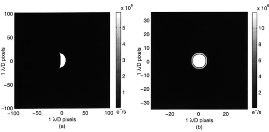
Figure 2-1: Earth images and e-/sec generated by Farzana Khatri's simulation for the MLCD mission with 1 A/D pixels, a) day 170 b) day 510

processing methods already being carried out, and no additional processing steps will be required. In searching for a surrogate data set, it was discovered that the 1994 Clementine mission to the moon did take several pictures of the Earth at 1 pm, and over a wide range of Earth phase angles [11]. This chapter will discuss how these images were used as a basis for generating simulated Earth image data in MATLAB on which to test the Earth-tracking algorithms.

2.1

Related Work

Farzana Khatri, a Lincoln staff member, previously created a MATLAB simulation of Earth phase and size in pixels for any given day of the Mars mission. The model produces a constant albedo surface and provides the photon flux from each Earth pixel assuming that constant surface. A sample image from Khatri's simulation is shown in Figure 2-1.

While a good starting point by taking into consideration the orbital dynamics of the mission, Khatri's simulation does not take into account the effects of the varying surface albedo or camera sensor parameters, and uses some generic optics character-istics as opposed to some more specific to the MLCD mission. The 1994 Clementine

Figure 2-2: Sample Clementine mission 1-Atm images of the Earth, taken from the

NASA Planetary Image Atlas [11]

mission to the moon took pictures of the Earth at our desired wavelength of 1 pim

+15 nm [11], a sample of which is shown in Figure 2-2.

These pictures were taken with a different camera (a Thomson TH7853-CRU-UV

Si CCD), from much closer to the Earth than Mars, and with higher resolution than

we will be expecting on the MLCD mission. However, these images could be used for

mapping albedo variations onto the Earth shapes generated from Khatri's simulation

if they are suitably rescaled to match the resolution of the MLCD Indigo ISC9809

camera. In addition, the MLCD team at Lincoln investigated the camera and sensor

characteristics to determine the relevant detector parameters. This thesis discusses

how these measurements were incorporated into Khatri's system model to correctly

simulate the effects of the camera and detector choice on the images.

Khatri's model also only produced single-point-in-time images, and no attempt

had been made to create image sequences of the Earth moving over a period of time.

Jamie Burnside, another Lincoln staff member, created a simulation of the open- and

closed-loop jitter expected to be seen during pointing and tracking operations of the

mission. Time sequences of the corresponding movements of the camera and thus

the Earth in the images were generated to match the jitter spectra of the mission,

and these time sequences were used in this thesis to generate moving Earth image

sequences.

2.2

Phenomenology

The rest of this chapter discusses the phenomenology of the MLCD mission and how each aspect of the system was modeled in the simulation.

2.2.1

Overview

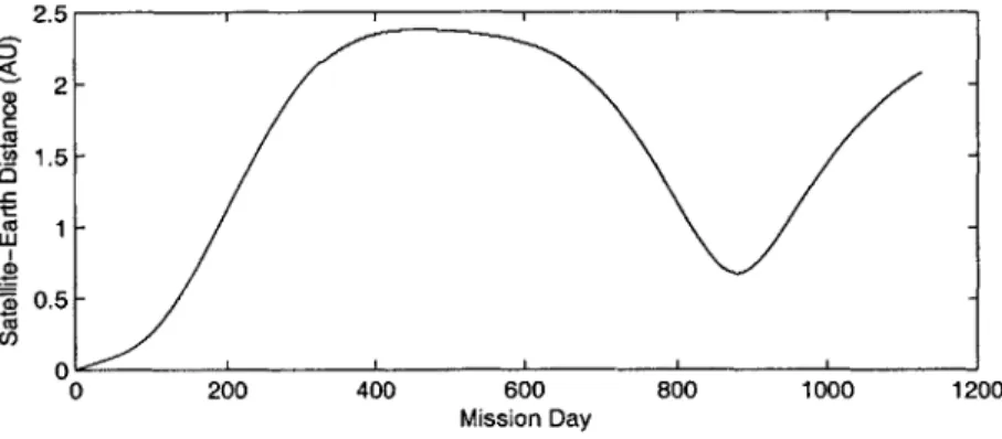
The anticipated launch date for the MTO satellite is October 6, 2009, with almost a year of cruise time before Mars orbit insertion (MOI) on August 29, 2010. It will subsequently remain in Martian orbit for up to 2 years, for a total mission lifetime of around 1100 days. There is a desire to be able to establish a communication link on most days of the mission for a few hours each day, both during the cruise and orbit phases of the mission. As such, a wide range of pointing and tracking situations for the satellite camera will be encountered over the course of the mission. The three main parameters governing the situation seen by the camera, the satellite-to-Earth distance, the Sun-Earth-Probe (SEP) angle, and the Sun-Probe-Earth (SPE) angle, are shown in Figures 2-3, 2-4, and 2-5, respectively, for the duration of the mission. The satellite-to-Earth distance determines the size of the beacon and Earth on the camera image and the signal power received from each, the SEP angle determines the Earth phase angle seen in the image, and the SPE angle determines how close the camera is to looking at the sun when trying to point at the Earth. MLCD requirements specify a desire to be able to establish a high rate communication downlink down to a 3* SEP angle and a 20 SPE angle.

At the beginning of the mission, the higher SEP angle indicates the satellite camera will see a crescent-shaped Earth. The Earth will still be fairly close, and until approximately day 160 of the mission, the beacon on the Earth will be strong and close enough to allow for high-bandwidth (i.e., up to 2 Hz) tracking on the beacon alone. As such, only the Magneto-hydrodynamic Inertial Reference Unit (MIRU) and other high-frequency systems and the beacon-tracking system will be in operation up to day 160 of the mission, the first crossover point. One thing to note is that during

0 200 400 600 Mission Day

800 1000 1200

Figure 2-3: Distance between MTO satellite and Earth throughout the mission

zUU (D 150-(D 100 50-U) 0 200 400 600 Mission Day 800 1000 1200

Figure 2-4: SEP angle between the Sun, Earth, and MTO satellite throughout the mission

200 400 600

Mission Day

800 1000 1200

Figure 2-5: SPE angle between the Sun, MTO satellite, and Earth throughout the mission 2.5 2 0.5 a) a.) C CO W) 100 80 60 40 20 a) ) C a) 0

this first part of the mission, there will be a point where the SPE angle drops below 20. Under such conditions, the camera will be looking almost directly into the sun, and the MLCD mission will not be required to point and track or establish a downlink during this time because of the expected high photon flux and the desire not to reach full well capacity in the camera pixels.

From day 160 until the second crossover point around day 810, the beacon will be too far away and thus too weak to be used for pointing all on its own. During the bulk of the mission therefore, both the Earth-tracking and low-bandwidth (up to 0.02 Hz) beacon-tracking systems will be in operation in addition to the high frequency stabilization systems, with the Earth-tracking system responsible for frequency dis-turbances between 0.02 and 2 Hz. During this time, the Earth will change in phase from a crescent to a full-disk shape at day 480, and then back to a crescent again, where the Earth is simultaneously at maximum range as a full disk and at closer ranges as a crescent. Again during this phase of the mission, there will be a point when the SPE angle drops below 20, and no pointing and tracking using the camera will occur at this time.

After day 810, there will again be a brief time when the Earth is close enough that beacon-tracking is sufficient. Finally, towards the end of the mission, the Earth-tracking system will again be needed when the third crossover point is crossed and the beacon becomes too weak for tracking on its own. Operational conditions during this period will be similar to those seen after the first crossover point at day 160.

Table 2.1 presents a summary of the different operating conditions for the lower frequency pointing and tracking systems throughout the mission.

2.2.2

From Earth to Camera Image

The processing steps for creating a simulation of Earth image sequences is presented in a conceptual block diagram in Figure 2-6. The orbital dynamics of the mission determine the size and shape of the sunlit Earth that would be seen by the spacecraft. Line-of-sight (LOS) jitter affects where the Earth lies in the field of view of the optics and camera system. As the photons of the Earth signal pass through the optics

Day Description of Conditions

0-160 Beacon-tracking system covers up to 2 Hz 74-77 SPE angle drops below 20, no camera tracking 160 First crossover point

160-810 Beacon- and Earth-tracking systems in use 324 Mars Orbit Insertion

480 Maximum range, full-disk Earth

480-495 SPE angle drops below 2', no camera tracking 810 Second crossover point

810-1000 Beacon-tracking system covers up to 2 Hz 1000 Third crossover point

1000+ Beacon- and Earth-tracking systems in use

Table 2.1: Summary of camera pointing and tracking systems' operating conditions

Solar Orbital Focal Camera

Irradiance and 1 Dynamics of LOS Optics - Plane - image

Earth Albedo Sun, Earth, Jitter Subsystem Array Frames

and Spacecraft

Figure 2-6: Conceptual block diagram for the Earth image simulation

subsystem, they finally land on the focal plane array of the camera. Electronic readout of the focal plane array provides the camera image frames that will be sent to the onboard processor for the Earth-tracking system.

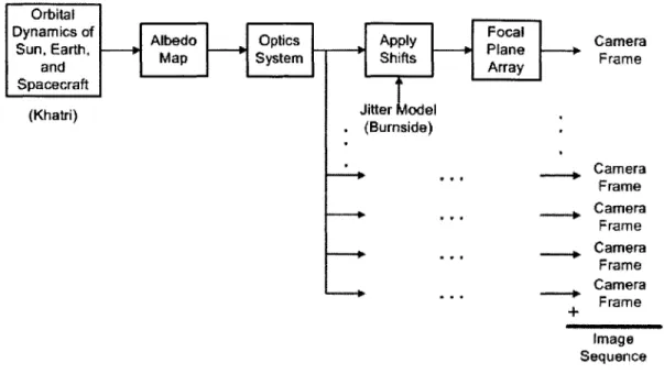
The actual implementation in MATLAB followed a different sequence of steps that is perhaps less intuitive to the reader, a block diagram of which is presented in Figure 2-7. This chapter will follow the implementation block diagram in the

discussion of the development of the Earth image simulation.

Khatri's simulation was slightly modified to provide a high resolution image of the constant albedo Earth disk. High resolution images were used because of the MATLAB processing steps required in the simulation of the optics subsystem and in the creation of image sequences from the jitter modeling step, as discussed later in this chapter. The Clementine mission images were resampled to match the resolution of these images and then mapped on to the Earth disks to add spatial albedo variations to the Earth's surface, as detailed in Section 2.2.3. The result of this step provides a

Orbital

A o Optcs Ay Fc Camera

andMap System Shifts ArrayFrame

Spacecraft Jte o e (Bumside) Camera Frame Camera Frame Camera Frame Camera Frame Image Sequence Figure 2-7: Implementation block diagram for the Earth image simulation

high resolution "image" of the expected photon flux arriving at the spacecraft. Once the photons from the Earth arrive at the spacecraft, they pass through the optics subsystem, the modeling and simulation of which is discussed in Section 2.2.4. At this point any "shifts" in the location of the Earth due to LOS jitter are applied to the image, using information from the jitter model created by Burnside and discussed in Section 2.2.6. After passing through the various optics system components, the photons from the Earth fall on the camera's focal plane array. The modeling and simulation of the conversion from photons landing on the focal plane array's detectors to the digital numbers and the image stored in memory is presented in Section 2.2.7. During this step the image is also downsampled back to the resolution of the camera. At this point, the simulation has generated one camera frame containing an Earth image that might be expected during the MLCD mission. To create successive camera frames, the next expected shift in the image as determined by the jitter model is applied to the output of the optics subsystem step, and passed to the focal plane array modeling block to create another camera frame.

Earth Surface Constituents % Reflectance at 1.06 prm

Clouds 67

Winter Snow and Ice 77

Summer Ice 46

Soil and Rocks 36

Vegetation 52

Water 7-12

Table 2.2: Percent reflectance at 1.06 pm of various Earth surfaces. Source: [14]

The major steps in the implementation of the Earth image simulation will now be discussed in the following sections.

2.2.3

Albedo Variations

The Clementine images were used to apply surface albedo variations to the Earth disks generated by Khatri's simulation of orbital dynamics. These images were taken using a i-pm imaging wavelength and thus had correctly scaled contrasts between the different Earth surfaces to match what would be seen during the MLCD mission. The intensity of each pixel in the Clementine images corresponds to an offset plus a gain times the average albedo of the Earth's surface being imaged by that pixel. Not knowing what these offset and gain coefficients might be to recover the albedo values, it was decided instead to perform histogram range adjustment on the images to make the brightest pixel correspond to the brightest possible Earth albedo and the dimmest pixel correspond to the dimmest possible Earth albedo, with all other pixels being scaled accordingly. Albedo values, or the spectral reflectance at 1.06 Am, of various Earth surface constituents are given in Table 2.2. Manual inspection of the rescaled images verified that different surface constituents were assigned reasonable albedo values using this method.

Once the Clementine images had been converted from camera intensity to Earth albedo values on each pixel, the images had to be resized to match the MLCD mis-sion. Bicubic interpolation was used to perform the resizing of the Clementine albedo images to have the same diameter as the corresponding high-resolution Earth disk

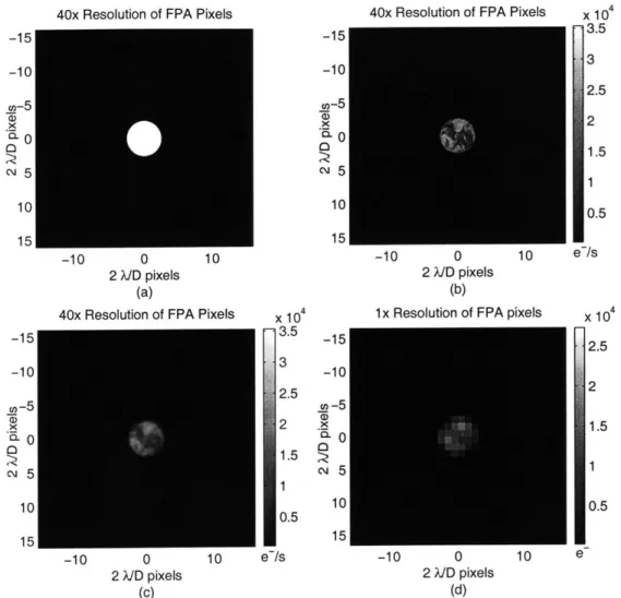
40x Resolution of FPA Pixels -15 -10 co-5 .0 CL0 c\i5 10 15 -10 0 10 2 AID pixels (a)

40x Resolution of FPA Pixels

-10 0 2 AD pixels (c) -10 0 10 2 AID pixels (b)

1x Resolution of FPA pixels x 104 35 r 10 e-/s -15 -10 co-5 0 c' 5 10 15 -15 -10 (-5 0 c 5 10 15 -10 0 2 AID pixels (d) 10 e

Figure 2-8: Simulated Earth image after each major processing block a) Modified

Khatri Orbital Dynamics block b) Albedo Mapping (with signal flux added) c) Optics

Subsystem d) Focal Plane Array

-15 3 -10 2.5 w-5 2 . 0 1.5 c 5 1 0.5 15 X 104 .. 3.5 S13 ,2.5 2 1.5 0.5 e /s x 104 2.5 2 1.5 1 0.5

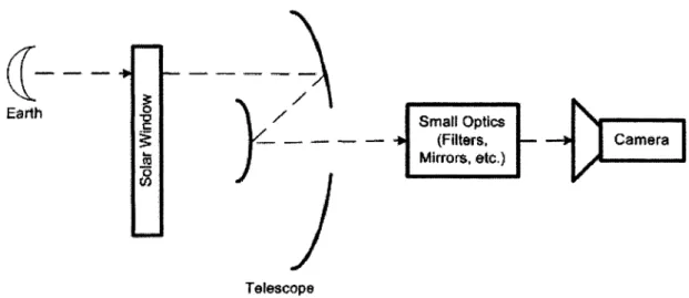
C---Er

Earth

I-9~ _{--- -} Small Optics_{(Filters, Cama}

Mirrors, etc.)

Telescope

Figure 2-9: The Optics Subsystem

calculated from the modified Khatri simulation, for any day of the mission. Once the albedo image was resized to match the appropriate Earth diameter for a given day of the mission, the Earth disk shape was used to mask out all but the section of the albedo image that lined up with the sunlit fraction of the Earth. Thus surface albedo variations were added to the high-resolution Earth shapes generated by the modified Khatri orbital dynamics simulation to create a high-resolution albedo image p(x, y).

2.2.4

Optics

A diagram of the components of the optics subsystem modeled in the simulation is shown in Figure 2-9.

Upon arriving at the optics subsystem of the spacecraft, the Earth signal first passes through the solar window filter. The filter has a 30-nm bandwidth centered around 1.06 jtm to limit the amount of stray sunlight entering the optics system. Light transmitted through the solar window next passes through the telescope's 30.5 cm diameter aperture. The Earth signal will be blurred by the telescope's Airy point spread function:

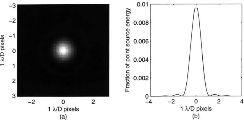
-3 0.01 ) -2: 0.008 a) 6 0.006 00 0.004 10 0 C .2 2 -j 0.002 3 0 -2 0 2 -4 -2 0 2 4

1 VID pixels 1 A/D pixels

(a) (b)

Figure 2-10: Airy point spread function for point source centered at (0,0) a) 2D point spread b) cross-section at y=O

Airy(x,

y)

r

where JI(r) is a first-order Bessel function, r is given by

r

r =

1/X2±+y2

and (x, y) is the position on the focal plane relative to the optical axis in units of A/D pixels. The scale factor (3.83/1.22) in r converts the location of the Bessel function zeros to their locations in units of diffraction-limited pixels. With such a point spread function, 86% of the energy from a point source would fall on one diffraction-limited pixel. Figure 2-10 shows a plot of the Airy point spread function of the telescope.

After passing through the telescope aperture, the Earth signal will pass through various small optics components, with 57.54% expected transmission of the Earth signal due to losses in the various components. Upon finally reaching the camera, the photons falling within the field of view of the camera will be detected with a quantum efficiency of 0.8.

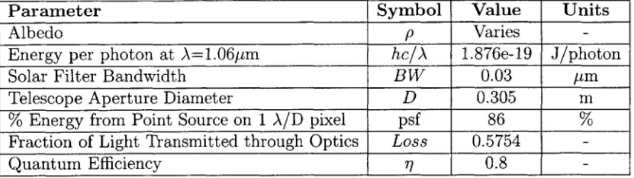
A summary of the optics subsystem parameters modeled in the simulation is presented in Table 2.3.

Parameter Symbol Value Units

Albedo p Varies

-Energy per photon at A=1.06pm hc/A 1.876e-19 J/photon

Solar Filter Bandwidth BW 0.03 pm

Telescope Aperture Diameter D 0.305 m

% Energy from Point Source on 1 A/D pixel psf 86 % Fraction of Light Transmitted through Optics Loss 0.5754

-Quantum

-Table 2.3: Parameter values for the optics subsystem

2.2.5

Signal Level

The Earth signal comes from sunlight reflected diffusely into space and imaged onto the focal plane array. The thermal emission from the 300-K Earth is negligible at 1 pm and is not included in the calculation of the Earth signal in this simulation. The sunlight reflected from the Earth's surface in [W/m 2_{] at our wavelength of interest is} given by

Reflected sunlight = p - Hx - BW. (2.2) where HA = 6.3 W/m2_{/pm is the solar irradiance on the Earth at 1 AU, centered at}

1.06 Iim, and p is the Earth albedo, which varies from 7% to 77% (see Table 2.2). The fraction of the solid angle of Earth light received at the MTO satellite tele-scope aperture over the total solid angle in which Earth light radiates is given by

7_ (D)2

Fraction light received = 2 , (2.3)

,7rR 2

where RME is the distance in meters between the Earth and Mars at the time the image is taken and the factor of 7r in the denominator comes from assuming the Earth can be modeled as a Lambertian surface.

Multiplying this fraction by the sunlight reflected from the Earth's surface gives the total Earth light in our wavelength band of interest falling on the telescope aper-ture in Watts per m2 of the Earth's surface. The amount of the Earth's surface being imaged is the area of the Earth multiplied by the fraction fE of the Earth that is

sunlit:

1

Area imaged = rR - (sin SEP

+

= 7rR2 -fE _(2.4)

where RE is the radius of the Earth in meters, and SEP is the Sun-Earth-Probe angle at the mission time for which an image is being simulated.

Combining equations 2.2 - 2.4 and adding in the other optics subsystem param-eters, the total Earth signal flux, SEarth, in [e/s] is given by

SEarth = HA - BW -R2 ) RE -7rfE - Loss - cY . (2.5)

RME) hC/A

This calculated SEarth assumes an average albedo p = 1, as in the constant albedo Earth disk shapes generated by Khatri's simulation. Dividing the SEarth signal flux

evenly among all pixels in the Earth shapes gives the signal flux per pixel of albedo

p = _{1. Multiplying this constant albedo signal flux image by the albedo image p(x, y)} from Section 2.2.3 gives an albedo image with appropriate signal flux, designated as

Sh(X, y).

Adding in the effects of the Airy point spread function of the telescope, the high resolution signal flux, Sh in [photons/s] on each high resolution pixel is given by the

2-D convolution:

Sh(x, y) = So(x, y) * Airy(x, y). (2.6)

2.2.6

Line-of-Sight Jitter

Line-of-sight (LOS) jitter in the imaging system is caused by random spacecraft mo-tion, resonance in the vibration isolators, and the excitement of discrete bending modes in the telescope. There are two elements to the effect that LOS jitter has on the camera images of the Earth. LOS jitter at frequencies higher than the frame rate

of the camera can cause smearing in the image taken in each camera frame. LOS jitter at lower frequencies causes the apparent shifts in the Earth's location between camera frames. The jitter can be analyzed by looking at it's simulated power spectral density or as a time series of expected LOS center movements. A plot of the LOS jitter spectra from Burnside's model is shown in Figure 2-11. A time series of ex-pected LOS movements according to the jitter model was also provided by Burnside to simulate Earth movements in the camera image simulation. Plots of sample time sequences fitting the jitter spectra are shown in Figure 2-12. Note that the LOS center shifts are given in units of diffraction-limited (1 A/D) pixels. This was done because the tracking accuracy requirement was given in units of A/D pixels, and it was desired to keep consistent the units of the pixel shifts applied to the Earth images and the accuracy requirement during algorithm testing.

In the simulation, the shifts in the Earth's location due to LOS jitter are applied after the optics step processing as if the shifts were only seen by the camera focal plane array, even though in the real system these shifts are seen by the entire optics system and thus "before" the convolution of the Earth light image with the Airy point spread function. This can be done because of the shift property of discrete-space Fourier transforms, yielding the same result whether the shift is applied to the Earth signal before or after passing through the telescope.

If

So(x,y)

then So(x -

x

y

Airy(x, y)

e- 2rf1xo e-32 f2yoShF fl f2),

and e-32fixoe-3 2

rf2yoShF fl, f

F2

As can be seen in Figure 2-12, the Earth-location movements expected are at the sub-limited-pixel level, on the order of a few tenths of a diffraction-limited pixel from frame to frame and on the order of a few hundredths of 0.1-0.2

5 01 100 10 102 Frequency (Hz) (a) 10 100 100 10 1 102 103 103 104 104 Frequency (Hz) (b)

Figure 2-11: Closed-loop LOS jitter spectra provided by Jamie Burnside a) x-direction b) y-direction N M10

N

_o

0.4 0.15 0.3 0.1 -L 0.2 - 0.05-0.1 0 a 0 -0.05 C/) aO 0 0 J -0.2 -0.15 -0.3' 02 -0.4 -0.2 0 0.2 0.4 -0.3 -0.2 -0.1 0 0.1 LOS x-center (1 VID pixels) LOS x-center (1 ?JD pixels)

(a) (b)

Figure 2-12: Sample LOS movements provided by Jamie Burnside in a) 1 s time period b) 4.8 ms time period. Note that the jitter is defined in units of 1 A/D pixels

diffraction-limited pixels within each 4.8 ms timeframe. As such, the camera pixel images would also have to be shifted at the subpixel level. Thus the high-resolution images were created to allow for "subpixel" shifts (which could be rounded to integer pixel shifts in high resolution images), because subpixel-level image shifting cannot be done without interpolation. The high-resolution images were formed from the beginning in the processing steps for simulating Earth images as opposed to after the optics processing block because of the lowpass filtering of the image by the telescope's point spread function. As opposed to performing interpolation and upsampling on a blurred version of the original "picture," the interpolation was performed on the original "picture" before being passed to the optics processing block. A sample camera frame image at this point in the simulation that includes the effects of smearing is shown in Figure 2-13. As can be seen in the figure, the effects of smearing are not significant enough to be visible to the human eye.

2.2.7

Focal Plane Array

Once the light hits the focal plane array, the sensor characteristics need to be taken into account. The pixel resolution governs the pixelation of the Earth signal and will determine the number of pixels across the Earth diameter in the image.

Diffraction-x 104 x 104 -15 .3.5 -15 .. 3.5 -10 3 -103 .D -5 2.5 -5 ,2.5 -155 S2 15. 2 1.5 ;Z 1.5 c 5 N 5 1

M1

2 AID pixels 2 AID pixels

(a) (b)

Figure 2-13: Sample camera frame image a) before smearing added b) after smearing

added

limited (A/D) pixels take advantage of the best resolution that the telescope can resolve and produces the finest detailed images. However, tradeoffs with other sensor characteristics call for a 2D pixel resolution to provide the best images for the overall camera tracking system. The photodetectors used in the focal plane array produce a dark current, B, a bias value that is present even in the absence of light and that will be added to any signal received on each pixel. There will be an integration time, T, associated with the camera to determine how long to integrate the photon flux from the Earth signal and the dark current in time in each frame. The signal on the detector also produces shot noise. Read noise, modeled as Gaussian with zero mean and -= ne = 160 e-/s, or .Nf(p = 0, -= n), is added to every pixel each time the

array is read out. For the focal plane array being used in the MLCD mission, the read noise is the dominant noise term. As such, the fewer pixels that need to be read out, the less noise there will be in the focal plane array system. Thus, 2A pixels were chosen to cut down on the number of pixels needed to read out the Earth image and thereby lessen the noise and increase signal-to-noise ratio. For each frame, only a 32x32 pixel area containing the Earth is read out. Finally, a 14-bit A/D converter with a quantization step of

Q

Parameter

Symbol

Value

Units

Pixel width pixel 2 A/D radians

Dark current B 200,000 e-/s

Frame Rate Fs 208 Hz

Integration Time T 1/208 s

Pixel Read Noise ne 160 e-/frame

A/D converter #bits b 14 bits

A/D converter quantization step

Q

focal plane array are summarized in Table 2.4.

The high-resolution Earth image, Sh(x, y), or its shifted version, is downsampled in this processing block to the resolution of the FPA by summing the signal in the area covered by each pixel to give the signal image S(x, y) in [e-/s]. The Earth image without noise in each frame is given by

S'(x, y) = (S(x, y) + B) -T. (2.7) The signal S' is a Poisson variable so its variance is the mean. The noise term added to each pixel based on the shot and read noise is given by

o-(x, y) = JS'(x, y) +

n

The number of electrons read out from each pixel is thus given by

Z(x,

y)

=

iV

(p(x, y)

=

S'(x,

_{y), o-(x, y)}

₌

_VS'(x,

y)+

n

,

The output of the focal plane array detector circuitry, Z(x, y) is then passed to the A/D converter, so that the final camera frame image used for the tracking system is given by

with the appropriate bound I(x, y) ; 2- -1 for all x and y, where 2b - 1 is the digital

readout of saturated pixels.

Sample images for various days of the mission are shown in Figure 2-14.

2.3

Limitations of the Simulation

2.3.1

Earth's Terminator

Real images showing the Earth's terminator (the day-night boundary on the Earth's surface) show a gradual transition from light to darkness, where the Earth seems to fade out as the boundary is crossed. This effect can be seen in the Clementine image shown in Figure 2-15.

These effects on the albedo image were not modeled in this simulation. The Earth shapes generated from Khatri's orbital dynamics simulation include the area where the terminator occurs, whereas the Earth albedo image is simply masked onto this shape from a full-disk image, with no additional adjustments made to handle the dimmer terminator. Although the albedo images could be processed by making adjustments based on the lighting conditions, perhaps by modeling the Earth as a non-Lambertian surface at low elevation angles, this processing was not done for this simulation. As a result, the simulated images show an abrupt transition from day to night on the Earth's surface with no fading on the terminator, as can be seen in the

Day 160 image in Figure 2-14.

2.3.2

Albedo Variations in Time

While in actuality the Earth's surface albedo changes over time, due to weather and the rotation of the Earth, the albedo images were kept constant in time in the Earth-image simulation. At the resolution and frame rate at which the MTO camera will be looking at the Earth, it was assumed that the albedo variations in time would be too small and too slow to change the images from frame-to-frame enough to affect the performance of the tracking algorithms. Thus, because the simulation is only meant

-10 0 10 2 V/D pixels (a) CL, C\J co C\IJ -10 0 10 2 VD pixels (e)

e

e

Lr

1

x

.a

0

0

e

e

e

Figure 2-14: Simulated Earth images a) Day 160 b) Day 200 c) Day 300 d) Day 479

e) Day 600 f) Day 808

e

I

I

.

Figure 2-15: Clementine image showing the Earth's terminator [11]

for generating short time sequences worth of data, the Earth's time-varying albedo was not modeled in the simulation, and the validity of this assumption was verified in Section 4.2 for the chosen tracking algorithm.

2.3.3

Angular Jitter

Besides the LOS jitter that makes the Earth appear to shift/translate across the camera field of view, the spin of the spacecraft adds rotation in the images. However, the rotation rate is too slow to be seen noticeably in the images at the frame rate being used by the camera, and its effects were not included in the simulation.

2.3.4

FPA Pixel Gain and Offset Non-Uniformity

One aspect of the focal plane array characteristics not included in the simulation was the non-uniform gain and offset associated with each photodetector in the conversion from photons to electrons. This non-uniformity will be compensated for through calibration during the mission to have a residual non-uniformity less than 0.02%. The effects of the residual non-uniformity on the tracking system were assumed to be insignificant and thus were not included in the simulation. For the purposes of the simulation, a uniform offset of 0 and gain of 1 were assumed across the FPA.

Chapter 3

Tracking Algorithms

Once simulated Earth image sequences were generated and the phenomenology of the system known, algorithms could be selected for the Earth-tracking system. As discussed in Section 2.2.6, the movements in the Earth's location from one frame to the next are expected to be at the subpixel level. Rotation and scaling will be insignificant in the frequency range and at the distances for which the Earth-tracking system is in operation. Between measurements of the Earth's absolute location from the beacon-tracking system, Earth albedo variations in time (due to weather patterns and the Earth's rotation about its axis), are also expected to be insignificant, and thus the albedo image mapped onto the Earth disk can be kept constant over successive camera frames. Determining the shift in the Earth's location between camera frames thus becomes similar to an image registration problem where the expected transformation from one image to the next is a pure, subpixel translation. The pointing requirements on the laser beam call for the Earth-tracking system to have a 0.089-diffraction-limited-pixel rms, 2-axis accuracy. The algorithm must also run within the 4.8 ms frame time along with other algorithms and processes that must be run each frame as well. This constraint on computational complexity is secondary to the accuracy requirement and could have been relaxed if no algorithms were found to meet both the accuracy and computational cost requirements. Fortunately, an algorithm was found that met both requirements. This chapter discusses the candidate subpixel image registration algorithms for the Earth-tracking system and the test results that