The effect of G-seat tactile cueing on linear motion perception

The Effect of G-Seat Tactile Cueing on Linear Motion

Perception

by

Patricia Barrett Schmidt

S.B., Aeronautics and Astronautics

Massachusetts Institute of Technology, 1996

Submitted to the Department of Aeronautics and

Astro-nautics in partial fulfillment of the requirements for the

degree of

Master of Science in Aeronautics and Astronautics

at the

MASSACHUSETTS INSTITUTE OF TECHNOLOGY

February, 1998

© 1998 Massachusetts Institute of Technology All Rights Reserved.

Author ...

...

..

.... ...

....

.

...

...

Departm

t

A'er nautics and Astronautics

//

;

December 9, 1997

C ertified by ...

...

... ...

Apo lo

Program Professor of Astronautics

Department of Aeronautics and Astronautics

SI Thesis Supervisor

A

ccepted by ... ...

. ...

.

"...

..

...

Jaime Peraire

Associate Professor

Department of Aeronautics and Astronautics

Chairman, Department Graduate Committee

The Effect of G-Seat Tactile Cueing on Linear Motion Perception

Patricia B. Schmidt

Submitted to the Department of Aeronautics and Astronautics on January 16, 1998, in partial fulfillment of the requirements for the

degree of Master of Science in Aeronautics and Astronautics

Abstract

Humans obtain information from several sources, including the vestibular system, vision, and tactile and proprioceptive sensation, in order to estimate spatial orientation. A model of this estimation process is particularly useful in flight simulation, where simulator cab motion, visual displays, and other devices are used to create an illusory perception of motion in pilots. Tactile cueing using G-seats has been used in flight simulation for z-axis acceleration and roll and pitch tilt cueing and has been shown to affect pilots' perceived motion. Although models describing the vestibular and visual roles in motion perception have been developed, the tactile contribution to motion perception, while significant, is less well understood. An experiment was conducted using a G-seat to quantify in the fre-quency domain the contribution of tactile cueing to linear motion perception. Eight blind-folded subjects were presented with uncorrelated sum-of-sines (.06 Hz-.5 Hz)

disturbances in horizontal velocity and G-seat pressure and used a hand controller to null the velocity disturbance. Half of the experimental trials used G-seat pressure and sled velocity disturbance, and the other half used only sled velocity disturbance. Transfer func-tions between sled velocity and control response (vestibular transfer function) and G-seat pressure and control response (tactile transfer function) were computed. Results showed a significant response to G-seat cueing, with a differentiator tactile transfer function. Small but significant increases in vestibular transfer function magnitude were seen when the G-seat was on. Differentiation in the tactile transfer function agrees with previous research on cutaneous tactile receptors and supports the use of the G-seat as an acceleration onset cueing device. The smaller than expected increases in vestibular transfer function magni-tude indicate that motion perception is not a simple sum of contributions from linear, time invariant tactile and vestibular estimators. A z-axis acceleration cueing drive algorithm for a pneumatic G-seat and a simulation concept using a pneumatic G-seat and a helmet-mounted display are proposed.

Thesis Supervisor: Laurence Young

Acknowledgments

I would like to thank Professor Larry Young for giving me the opportunity to work on this project and for providing the guidance that made this thesis possible.

I would also like to thank Dr. Billy Ashworth at NASA Langley Research Center for the loan of the G-seat used in this work.

Many thanks are due to Mike Markmiller, for building the hardware that allowed the G-seat to work on the sled, and most importantly, for trusting a UROP student to do "important" work, and teaching me about everything from soldering to pipe fittings.

I am indebted to Sherry Mowry and Nasos Dousis for their help in experiment devel-opment.

Special thanks go to students at the MVL, for making life around here interesting. Thanks to Jen, who knows why the sky is red at sunset but blue at noon, to Keoki for advice and Mardi Gras parties, to Dawn for that awesome banana bread and for putting up with silliness, to Amir for interesting conversation and computer help, and to Prashant for musical entertainment.

Thanks to Marsha Warren, for taking care of all the paperwork and red tape. A big thank you to Dick Perdichizzi and Don Weiner for technical assistance. Special thanks to Subjects A through N for their time and cooperation, which was uncompensated except for one 44 ounce raspberry slurpee.

I owe a huge debt to my parents for making it possible for me to come to MIT, and to Julie and Harry for their support. Thanks to all of my friends from House 4, especially

Karen and Rich, my teammates from the sailing team, Hatch and Fran, and the GNC4

crew, for keeping me sane through five and a half years at MIT. This work was funded by NASA Grant NAGW-3958.

Table of Contents

2.2 Tactile receptors in the skin ... 11

2.3 Models of spatial orientation ... ... 12

2.4 Previous G-Seat Research... ... 13

3 E quipm ent ... ... 16

3.1 G -seat ... . . . ... 16

3 .2 S led ... ... 20

3.3 Subject's Hand Controller...22

3.4 Data Acquisition ... ... 23 3.5 Command Generation ... ... 24 4 E xp erim ent ... 2 6 4.1 Overview ... 26 4.2 D isturbance Profiles ... 27 4.3 Experiment Design... ... 30 4 .4 Subjects ... ... 33 4.5 Experiment Procedure...34 5 D ata A nalysis ... ... 35 5.1 O verview ... 35

5.2 Derivation of transfer functions ... 35

5.3 Transfer function calculation ... ... 40

5.4 Significance of tactile transfer function magnitudes ... 41

5.5 Transfer function fits...42

6 R esults ... ...44

6.1 Computed transfer functions ... 44

6.2 Comparison between G-seat on and off conditions ... 48

6.3 Fitted transfer functions ... 51

7 D iscu ssion ... ... 57

7.1 Influence of G-seat on motion perception ... ... 57

7.2 Tactile transfer function ... 57

7.3 Vestibular transfer function ... ... 61

7.4 G-seat drive algorithm ... ... 61

7.5 Pneumatic G-seat in flight simulation... ... 63

8 Conclusions and Recommendations for Future Work ... 65

8.1 C onclusions ... 65

8.2 Recommendations for Future Work... 66

9 R eferences ... ... 67

Appendix A Consent Form and Subject Instructions...69

Appendix B Practice Disturbance Profiles... 71

Appendix D G-seat checklist ... 74

Appendix E Matlab Scripts ... 76

List of Figures

Figure 3.1: G -seat... . . ... 16

Figure 3.2: G-seat frequency response (Markmiller 1996)...18

Figure 3.3: G-seat step response ... 19

Figure 3.4: M IT sled ... ... 20

Figure 3.5: Data acquisition and command schematic ... .. 23

Figure 3.6: Labtech data display window ... .... 24

Figure 4.1: Experiment Block Diagram...27

Figure 4.2: Sample sled velocity disturbance profile... ... 29

Figure 5.1: G-seat on block diagram ... 36

Figure 5.2: G-seat off block diagram ... 38

Figure 6.1: Mean vestibular transfer function, G-seat off ... 45

Figure 6.2: Mean tactile transfer function, G-seat off ... 45

Figure 6.3: Mean vestibular transfer function, G-seat on ... 46

Figure 6.4: Mean tactile transfer function, G-seat on ... 46

Figure 6.5: Mean transfer function, eyes open ... 47

Figure 6.6: Mean over all subjects, tactile transfer function comparison ... 50

Figure 6.7: Mean over all subjects, vestibular transfer function comparison ... 51

Figure 6.8: Tactile transfer function mean for subjects D, F, I, and L ... 52

Figure 6.9: Tactile transfer function mean for subjects E, H, J, and K...53

Figure 6.10: Tactile transfer function mean over all subjects...54

Figure 6.11: Fitted vestibular transfer function, G-seat on ... 55

Figure 6.12: Fitted vestibular transfer function, G-seat off ... 56

Figure 7.1: Block diagram for scheme 1...59

Figure 7.2: Block diagram for scheme 2... ... 60

List of Tables

Table 4.1: D isturbance profiles... ... 29

Table 4.2: Ordering of trials in experiment profile... ... 32

Chapter 1

Introduction

1.1 Motivation

The human brain combines information from a number of sources to obtain an esti-mate of the body's orientation and motion. The two major sources of information are the vestibular system and vision, while additional contributions are made by tactile and prop-rioceptive sensation. A considerable amount of research has been done to model the rela-tive contributions of visual and vestibular information; however, tactile sensation has recieved relatively little attention in motion estimation modeling efforts. (Borah, Young, and Curry 1978)

Motion sensation through tactile cueing recieved attention beginning in the 1970's as a method of providing additional motion cueing in flight simulation. Flight simulators use a combination of simulator cab motion and visual scene motion to convey to the pilot the motion of the simulated aircraft. (Rolfe and Staples 1986) Tactile stimulation was investi-gated as a way of providing the sustained linear acceleration cues that simulator cab motion and visual field motion could not reproduce. (Kron 1980)

The device used in flight simulators to produce tactile cues in the simulator is known as a G-seat. A G-seat is a flight simulator seat which has inflatable cushions or hydrauli-cally actuated panels in the seat pan and back. By altering the pressure distribution on the skin of the pilot's back and legs, the G-seat mimics the tactile stimulation produced by contact between the pilot and seat in an accelerating aircraft. Several versions of the G-seat were developed.(Kron 1980) Drive algorithms for G-G-seats were developed to produce tactile cueing for z-axis acceleration and roll and pitch tilt.(Flach, Riccio, McMillan, War-ren 1986, Martin, Osgood, McMillan 1987)

The majority of research on the G-seat has focused on its role in simulation, specifi-cally on the performance of pilots in flight simulators using the G-seat. In order to incor-porate tactile sensation into overall models of spatial orientation, a broader understanding of motion sensation through tactile cueing is needed. The objective of this study is to assess the effectiveness of a G-seat at producing illusory linear motion outside of a flight simulation environment and to quantify the contribution of G-seat tactile cueing to linear motion perception.

1.2 Organization

Chapter 1 describes the motivation for this work. Chapter 2 discusses background infor-mation about the motion perception process and the G-seat. Chapter 3 describes the equip-ment used in the experiequip-ment and Chapter 4 describes the design and execution of the

experiment. Chapter 5 details data analysis, and Chapters 6, 7 and 8 contain the results,

Chapter 2

Background

2.1 Vestibular System

The vestibular organs, which are located in the inner ear, are the primary motion sensors in humans. The semicircular canals sense angular velocity, while the otolith organs sense lin-ear acceleration, which may be caused by tilt with respect to gravity, linlin-ear motion. or cen-trifugal acceleration. Fernandez and Goldberg (1976) found that the otolith organs respond to tilt and centrifugal acceleration, by recording from individual otolith neurons.

2.2 Tactile receptors in the skin

The skin contains a variety of specialized receptors which sense touch, heat, cold, and pain. Two types of touch receptors are found in hairy skin: slowly adapting and rapidly adapting receptors.

Slowly adapting receptors sense a sum of velocity and position of skin indentation and stretch. Morphologically and functionally, they fall into two categories. The Type I recep-tors, or Merkel cells, are found in the epidermis and code a combination of position and velocity of skin indentation. (Burgess and Perl 1973) Linear systems analysis of the response of single Type I receptors shows that the receptors have a fractional integrator transfer function, as a result of their nonlinear dynamics. (Looft and Baltensperger 1990)

Type II receptors, or Ruffini endings, are found in the dermis. Type II receptors are stimulated by lateral stretch of the skin and code a combination of stretch and stretch rate. (Burgess and Perl 1973)

Rapidly adapting mechanoreceptors in the skin, such as the Pacinian corpuscle, sense vibration. The multi-layered corpuscle which surrounds the nerve ending acts as a mechanical high-pass filter, only transmitting velocity and acceleration of skin

indenta-tion.(Loewenstein 1971) Because Pacinian corpuscles respond to skin indentation velocity and acceleration with a high threshold, they are considered to be vibration transduc-ers.(Burgess and Perl 1973)

2.3 Models of spatial orientation

Several models have been developed to describe the motion estimation process in humans. These models primarily deal with motion estimation from visual and vestibular inputs, although one model (Borah, Young, and Curry 1978) includes tactile and proprio-ceptive inputs.

Zacharias (1977) proposed a linear estimator model and conducted experiments to determine the estimator transfer functions for the visual and vestibular systems in yaw rotation. Subjects in Zacharias's experiment controlled yaw rotation of a flight simulator while viewing a moving visual surround. Zacharias found that the linear estimator model did not fit the experimentally determined transfer functions and proposed a non-linear model, known as the conflict model, in which the visual and vestibular signals are aver-aged with a weighting that is determined by the amount of conflict between them. For short duration conflict, the weighting is shifted toward the vestibular signal. He used com-puter simulations of his model to demonstrate that it fit his experimental data.

The Zacharias conflict model was strictly designed to fit experimental data, but a model based on optimal estimation can be derived from first principles, given information about the sensors. Oman (1982) proposed an estimator model which uses a Kalman filter, an estimator which is optimal for a particular set of sensor noise covariances.

Borah, Young, and Curry (1978) simulated a steady-state Kalman filter model, but found that it was necessary to add the conflict nonlinearity of Zacharias's model in order for the results to agree with experimental time response data. The constant-gain Kalman

filter alone did not reproduce the delay in onset of circularvection when a stationary sub-ject is presented with a rotating visual scene, but the combined Kalman filter-conflict

model did reproduce the time delay.

Merfeld (1990) conducted an experiment with monkeys on a centrifuge, recording tor-sional eye movements in response to the changing gravito-inertial vector. He developed a linear model for estimation of the direction of the gravity vector, with estimator gains set to match experimental data. One important difference between Merfeld's model and pre-vious models was that his model used quaternions to represent angles in three-dimensional space. This allowed the model to be give accurate results with large deviations from cen-ter.

Pommellet (1990) proposed a time-varying extended Kalman filter estimator model for spatial orientation, using only vestibular inputs. Pommellet's model used quaternions to represent spatial orientation. Since the quaternion representation introduced nonlinear-ities, Pommellet's estimator applied the Kalman filter equations to a representation of the system dynamics that was linearized about the value of the estimated state at each time step. This type of estimator is known as an extended Kalman filter. Model outputs were found to agree qualitatively with data from Merfeld's experiment in some cases, but in other cases, the model's estimated state converged much more quickly to the true state than Merfeld's experimental results would indicate.

2.4 Previous G-Seat Research

One of the earliest G-seats was built at NASA Langley Research Center and integrated into Langley's Differential Maneuvering Simulator. The Langley G-seat was intended for normal acceleration cueing only. It had eight inflatable bladders, arranged in 2 by 2 arrays on the seat pan and back. The drive algorithm for the Langley G-seat was based on contact

between the pilot's ischial tuberosities and the hard base under the inflatable cushions and required the pilot to be loading the seat pan with his or her weight. For the zero accelera-tion condiaccelera-tion, the cushions were inflated so that the pilot's weight was mostly supported on a cushion of air, with some of the force transmitted through the ischial tuberosities (ITs) to the rigid seat base. In order to simulate headward acceleration, air was let out of the cushions, causing more of the pilot's weight to be supported by the ITs in contact with the hard seat base. To simulate footward acceleration, the cushions were inflated, causing the pilot's weight to be supported by the cushions, rather than contact between the ITs and the seat base. Initial reports by pilots indicated that the tactile cues produced by the G-seat were realistic.(Ashworth 1976) Further testing of the Langley G-seat demonstrated that pilots' performance using the G-seat in fixed-base flight simulation was better than their performance without the G-seat. (Ashworth, McKissick, Parrish 1984)

The next generation of G-seats was the Advanced Low Cost G-Cueing System (ALCOGS), which was developed by the Link Division of Singer Corporation for the Air Force. The ALCOGS G-seat had a seat pan driven in heave, pitch and roll by hydraulic actuators, which was overlaid with pneumatic firmness bladders. The backrest of the seat was hydraulically driven in roll, pitch and heave, while panels located in the lower corners of the backrest were extended and retracted. The ALCOGS design addressed several shortcomings of the pneumatic G-seat. The hydraulic actuators had a higher bandwidth and less time delay than the pneumatic G-seat, and, unlike the Langley G-seat, the height and firmness of the seat pan could be independently controlled. (Krohn and Kleinwaks,

1978)

Extensive research was done to develop roll and pitch drive algorithms for the ALCOGS. Contrary to researchers' expectations, drive laws based on roll velocity and position resulted in better pilot performance than drive laws based on roll acceleration.

(Levison, McMillan, Martin, 1984). Later drive algorithms were developed using psycho-physical matching techniques. (Flach, Riccio, McMillan, Warren, 1985) Comparisons between pilot performance using visual cues alone, the ALCOGS alone, and the combina-tion of ALCOGS and visual cues showed that use of the ALCOGS alone resulted in better pilot performance than the use of visual cues alone. (Snell, Flach, McMillan, Warren,

1985)

Research on tactile cueing of motion at MIT has focused on the relative contributions of tactile, vestibular and visual cueing to motion perception, using a Langley G-seat. Markmiller (1996) conducted an experiment in rostro-caudal axis linear motion, analo-gous to Zacharias's (1977) experiment, using a G-seat and head-mounted display on the MIT sled. Subjects controlled the sled with a hand controller, and their task was to null out a sum-of-sines velocity disturbance, with additional sum-of-sines stimuli presented in the visual field and G-seat. Transfer functions for each of the channels were calculated using a cross-correlation method similar to that proposed by Zacharias (1977).

Chapter 3

Equipment

3.1 G-seat

The G-seat is a flight simulator pilot's seat with inflatable cushions on the seat pan and back. The seat used in this experiment, which is shown in Figure 3.1, is a Langley G-seat, as described in Section 2.3, and is pneumatically driven.

Figure 3.1: G-seat

The seat pan, which was the only portion of the G-seat used in this experiment, con-sists of a 2x2 array of cloth-covered silicone rubber air bladders on a wooden seat base. A pressure transducer is mounted on each air bladder. The dimensions of the seat pan with the G-seat inflated are 14" (35.6 cm) by 16" (40.6 cm) by 6" (15.2 cm). At maximum inflation of the unloaded seat, the cushions are approximately 1.5 " (3.8 cm) in thickness.

One inch diameter steel pipes connect each air bladder to a pipe nipple which extends out the back of the wooden seat base. These pipe nipples are connected by 10 foot (3.05

m) length, 1" (2.54 cm) diameter rubber hose to a valve assembly located under the sled cart. The valve assembly consists of four anti-G-suit valves, actuated by Ling Model 203 shaker motors. The anti-G-suit valves are spool valves which have two positions: open or closed.

Bottled nitrogen was used as the gas supply for the G-seat. Nitrogen was supplied to

the G-seat's valve manifold, through a 40 foot (12.2 m) rubber hose at 80 psi (544 kPa),

where a regulator on the valve assembly reduced the pressure to 5 psi (34.0 kPa). The long

hose was necessary so that the nitrogen cylinder could be secured to the lab wall. The nitrogen at 5psi was then supplied to the four anti-G-suit valves which regulated gas flow into the G-seat cushions.

The G-seat control system is an analog pressure controller, which separately controls pressure in each of the four seat cushions. Seat cushion pressure is measured with a National Instruments Model LX1802GN pressure transducer on each seat cushion. The pressure signal is inverted and low-pass filtered, then summed with the command signal and a user-adjustable bias to form the motor drive signal. The motor drive signal goes to a set of motor amplifiers (Inland Motor EM 1802) which power the motors. A terminal on the G-seat controller chassis allows the low pass filtered pressure signal to be monitored and recorded by a computer.

The control system has several user-adjustable parameters, which are set with potenti-ometers on the controller boards. They include a pressure signal bias, pressure signal gain, command signal gain, and motor drive signal bias. These gains and biases were set so that the pressure signal is zero when the cushions are not inflated, and the responses of the two front and two back cushions match each other.

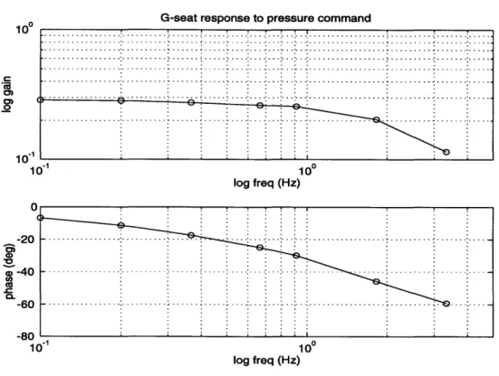
The simplicity of the G-seat control system presented two possible problems. The first potential difficulty, which was addressed by Markmiller (1996), was low bandwidth.

Markmiller experimentally determined transfer functions from command to cushion pres-sure and command to cushion displacement, demonstrating that the G-seat's bandwidth was adequate for a manual control experiment. A bode plot of the G-seat system's response to sinusoidal pressure commands is shown in Figure 3.2

G-seat response to pressure command

100 10 10 100 log freq (Hz)

o

-40

Figure 3.2: G-seat frequency response (Markmiller 1996)

The second potential difficulty was the possibility of a long time delay in the G-seat's response to commands. Markmiller's G-seat transfer functions did not indicate a signifi-cant time delay. This was confirmed by testing the response to a step pressure command. Figure 3.3 shows the result of the step response test. Figure 3.3 shows a two-sample delay between pressure command and pressure, which corresponds to a time delay of 20-40 msec.

1 0.8 0.6 0.4 0.2 0 -0.2 -0.4 -0.6 -0.8 -1 12

G-seat step response

SI I I I o Pressure x Commanded pressure ... ... . .. . . . . . . . I . I. . . . . .I.. . . . . ._{.. . . ..-. . . . .}. .. _{-) . . . .. . .}...._{. . . .}E) ( ... .. . . ..-. . . .. . . . .7 12.8 12.9 13 Time (sec) 13.1 13.2

Figure 3.3: G-seat step response

One issue that arose during testing was the need for an acceleration feedforward gain to the G-seat. The G-seat pressure control system obscures the normal tactile cues that a subject receives when the sled is in motion. As the sled accelerates in the headward direc-tion, pressure increases in the G-seat, due to the inertial force of the subject's body on the seat. As a result, the controller lets gas out of the cushions, in order to return the pressure to its commanded value. Footward acceleration of the sled produces the reverse effect, as the seat inflates to maintain a constant pressure. This effect results in the subject sinking into the seat and rising out of it by an abnormally large amount when the sled moves. To counteract this unrealistic effect, sled acceleration was fed forward to the G-seat command signal, in order to raise the commanded pressure when sled acceleration was in the head-ward direction and lower the commanded pressure when sled acceleration was in the

foot-19

.3

ward direction. The feedforward gain was selected based on a subjective assessment of the realism of the seat's motion during sled motion.

3.2 Sled

The MIT sled, pictured in Figure 3.4, is a human-rated linear acceleration cart. It has a reorientable subject chair on a cart which moves along two parallel rails. The range of motion of the sled is 4.7 m from one end of the track to the other.

Figure 3.4: MIT sled

The subject seat is enclosed in a fiberglass and aluminum frame. This chair assembly can be oriented for motion in one of three axes: rostro-caudal (z-axis), inter-aural (y-axis), and anterior-posterior (x-axis). Three restraints are provided for subjects: a five-point air-craft harness, an adjustable head restraint made up of padded plexiglass blocks, and nylon straps to restrain the feet on the footrest. Cloth was draped around the outer frame of the seat assembly, in order to prevent subjects from sensing sled velocity through wind cues.

An intercom is provided for two-way voice communication between the subject and the sled operator.

The sled is driven by an Inland Motors permanent magnet servo motor. The motor turns a 1 foot diameter aluminum drum, which drives a steel cable. The cable makes a complete loop between the drum, the sled cart and an idler at the opposite end of the track. The motor is controlled by a GE HiAK pulse width modulation controller.

The sled is commanded by a Northgate 386 PC computer running "sled", a C++ pro-gram written specifically for the MIT sled. The computer also outputs an auxiliary com-mand signal, which was used to comcom-mand the G-seat. The sled software allows the user to set up and execute experiment protocols for both the sled and the auxiliary device.

One issue of concern in this experiment was the likelihood of the sled reaching the end of the track during an experiment run. Several mechanisms exist to prevent injury or dam-age if the sled hits the end of the track. First, the sled program incorporates a position lim-iting algorithm which sets the commanded sled velocity to zero if the sum of sled's position and a constant multiplied by velocity exceeds predetermined limits. Second, limit switches are located at either end of the track. The limit switches are triggered when the sled cart comes in contact with them, interrupting a circuit which activates the brake, bringing the sled to a rapid stop. Third, bungee cords and steel bumpers are positioned beyond the limit switches to stop the sled should the limit switches fail. Finally, the opera-tor can either command zero velocity ("Soft Abort") or activate the brake ("Hard Abort") from the operator's console and the subject can activate the brake by pressing the subject's stop button at any time during the run.

In an early experiment run, it was discovered that a failed isolation amplifier in the sled operator's console prevented the sled computer from receiving sled velocity data. Because of the amplifier failure, the sled velocity signal at the computer was a constant -15 volts,

and the velocity input to the position limiting algorithm was a large negative value. As a result, the position limiting algorithm stopped the sled approximately 10cm short of the end of the track on the negative side, and did not stop the sled before it reached the limit switch on the positive side of the track. Because of the other safety mechanisms described above, the lack of a computer-controlled position limit at one end of the track was not con-sidered to be a serious problem.

3.3 Subject's Hand Controller

Subjects controlled sled velocity using a sliding hand controller which was constructed specifically for sled-G-seat experiments by Markmiller (1996). The controller is a rectan-gular box (10"x5"x3") (25.4 cm x 12.4 cm x 7.62 cm) with a knob on the right side of the box. The knob slides parallel to the axis of motion of the sled. Rubber bands return the knob to the center when it is released. The controller is mounted on the sled chair frame so that the knob is located 22 inches (55.9 cm) above the seat backrest. The controller has a range of motion of 8.5 inches (21.6 cm), and an output range of -15 volts to +15 volts. Headward motion of the controller commands headward motion of the sled.

The controller signal is filtered by an analog filter (Krohn-Hite Model 3340) with a cutoff frequency of 40 Hz. The control signal is then multiplied by a gain and low-pass fil-tered digitally in the sled program. The control signal gain is set based on the maximum velocity in the sled disturbance profiles, using a method developed by Hiltner (1981). The gain is set so that the velocity commanded by 90% deflection of the subject's controller is equal to the highest disturbance velocity. This algorithm resulted in a control signal gain of .113. The digital low-pass filter has a cutoff frequency of 10 rad/sec.

3.4 Data Acquisition

Data was acquired on a 90 Mhz Pentium PC computer, running Labtech 9.0, using a Kei-thley Metrabyte DAS-1600 data acquisition board. Four channels of analog signals were recorded: pressure in G-seat cushion #1, sled acceleration, sled velocity, and the subject's

command signal. Pressure data came from the pressure output port on the G-seat control-ler chassis and was low-pass filtered by an analog circuit to attenuate high-frequency noise caused by the G-seat servo amplifiers. Acceleration was measured by a Setra model 110 accelerometer mounted to the sled cart. Velocity was obtained from the tachometer on the sled motor, and the subject's control signal was recorded at the point where it entered the sled operator's console. A schematic of data acquisition and command for the experiment

is shown in Figure 3.5.

Pressure --- Command

r--- _{---- Data}

G-seat

- - Pentium command _Pressure

lr - Computer G-seat ...

I I Subject

I I Sled '*A cmlr a i

Sled command Sled Acceleration

I Computer

Velocity

P

I

Acceleration

Figure 3.5: Data acquisition and command schematic

Because of the isolation amplifier failure in the operator's console, the velocity signal was not available from the velocity output port on the console. The velocity signal was obtained by tapping into the signal where it entered the console, then buffering it with a unity-gain amplifier and connecting the buffered signal to the computer, thus bypassing

the failed component in the console. The resulting velocity data was more noisy than nor-mal, but the noise was filtered out of the recorded data adequately in Matlab.

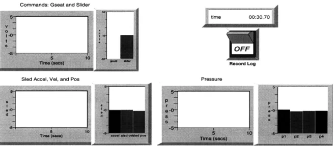
The Labtech software acquired data at a 50 Hz sampling rate, displayed, and recorded

it. The Labtech data display window is shown in Figure 3.6. Data files were named as

fol-lows: <subject><trial number>; for example, ell is subject E, trial number 11. Subject

designators for subjects A, I, and J were aa, ii, and

jj,

vari-able names. The data files were saved in five-column ascii format, where the columns were time in seconds, pressure, acceleration, velocity, and control signal. Labtech appended an end of file character to the end of each data file, which had to be removed before loading the file in Matlab.

Commands: Gseat and Slider

time 00:30.70

Record Log

Sled Accel, Vel, and Pos Pressure

Figure 3.6: Labtech data display window

3.5

Command Generation

Commands to the G-seat originated from both the Pentium and the sled computer. The auxiliary command signal from the sled computer was used to command a sum of sines pressure profile for the G-seat, and the Pentium computer was used to command the

accel-eration feedforward which was described in Section 3.1. The accelaccel-eration feedforward command, which was the measured sled acceleration multiplied by a gain, was output using a Keithley Metrabyte DDA-16 analog output board. The two command signals were summed using an analog summer, and the total command signal was connected to the "command in" port on the G-seat controller chassis.

Commands to the sled were generated by the sled computer and originated from two sources: the sum of sines disturbance profiles and the subject's commands. The sled dis-turbance profiles are discussed in section 4.2. The subject's commands were low-pass fil-tered and multiplied by a gain, as described in Section 3.2, and summed with the disturbance profiles to result in the total command to the sled.

Chapter 4

Experiment

4.1 Overview

The goal of this experiment is to determine whether tactile cueing using a G-seat affects linear motion perception and to quantify its contribution in the frequency domain. The experiment design is patterned after two experiments with similar goals, done by Zacharias (1977) and Hiltner (1983). Zacharias conducted an experiment in yaw rotation in which subjects viewed a visual display and were instructed to null out a sum-of-sines disturbance in their yaw velocity. The visual display indicated their true angular velocity plus a sum of sines disturbance. Hiltner (1983) developed protocols for a velocity nulling experiment using the MIT sled, and demonstrated that blindfolded subjects could null out a sum of sines linear velocity disturbance on the sled.

The experiment is a closed-loop velocity nulling task. Blindfolded subjects are seated on the sled and given a sum of sines disturbance in sled velocity and G-seat pressure. Their task is to use a hand controller that commands velocity to null out the sled's velocity.

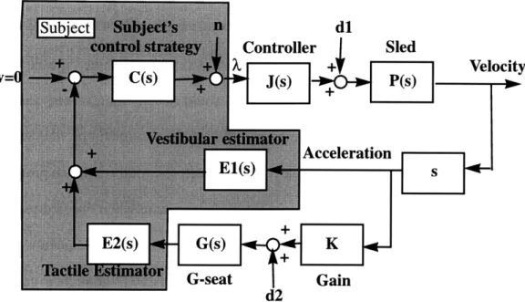
Figure 4.1 is a block diagram representation of the velocity nulling task in the experi-ment. The shaded portion of the block diagram indicates the estimation and control pro-cesses that occur in the human operator, and the unshaded portion indicates the dynamics of the subject's controller, sled and G-seat. The two disturbances given to the subject are dl, the sled velocity disturbance, and d2, the G-seat pressure disturbance.

Figure 4.1: Experiment Block Diagram

4.2 Disturbance Profiles

The disturbances provided to the subjects must meet requirements imposed by the human operator, the sled and the G-seat. The disturbance must be unpredictable, in order to evoke realistic disturbance rejection control responses from the subject. Since the human opera-tor's bandwidth is limited, the disturbance must be limited in bandwidth to below

approx-imately .5 _{Hz. Profiles must also minimize the amount of time spent at sub-threshold}

accelerations. The disturbance is also subject to limitations on maximum sled position and maximum G-seat pressure.

Hiltner (1983) demonstrated that subjects could perform a velocity-nulling task on the MIT sled. Since the disturbance profiles used in Hiltner's experiment met the necessary conditions, they were adapted for use in this experiment.

Hiltner's disturbance profiles were the sum of sines at 12 different frequencies. The frequencies are prime multiples of a base frequency of .01221 Hz. so that no frequency is

a harmonic of another. The phase difference between sines at successive frequencies is a

constant, 253 deg., in order to avoid a large disturbance magnitude at the start of the trial.

Hiltner's sled velocity profiles were determined according to three criteria: sled dis-placement constraints, minimum time at sub-threshold acceleration levels, and subject performance. Hiltner iterated on relative magnitudes of sines to obtain profiles with mini-mum time at sub-threshold acceleration levels and selected several candidate protocols for testing with human subjects. Since experiment trials terminate when the sled reaches the end of the track, it is essential to determine that the subjects can adequately null sled velocity for a particular sled disturbance profile. The profiles with the highest completion rates were selected for use in the experiment. (Hiltner 1983)

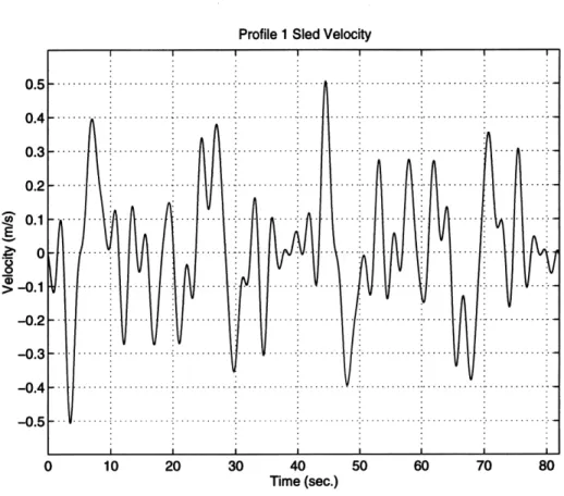
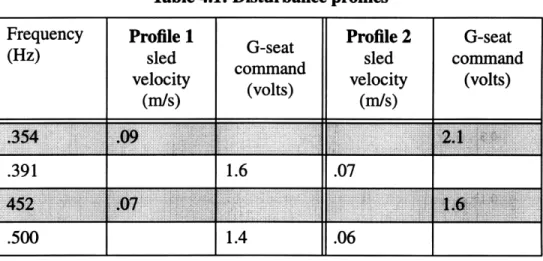
Since this experiment used two disturbance modalities, sled and G-seat, sines at 6 of the 12 possible frequencies are used for each channel, alternating between sled and G-seat. This results in two disturbance profiles. Profile 1 has sled disturbance at odd-numbered frequencies and G-seat disturbance at even-numbered frequencies. Profile 2 has sled dis-turbance at even-numbered frequencies and G-seat disdis-turbance at odd-numbered frequen-cies. The frequencies and magnitudes of the sled and G-seat disturbance profiles are shown in Table 4-1. One of the sled disturbance profiles is shown in Figure 4.2

Data from both profiles is required for computation of vestibular and tactile transfer functions. A group of two trials using Profile 1 and Profile 2 is the smallest unit of data that can be analyzed. This group of trials referred to as a block

Profile 1 Sled Velocity 0.1 0 > -0.1 0 10 20 30 40 50 60 70 80 Time (sec.)

Figure 4.2: Sample sled velocity disturbance profile.

Table 4.1: Disturbance profiles

Frequency (Hz) Profile 1 sled velocity (m/s)

1

₁

I

I

Table 4.1: Disturbance profiles

Frequency Profile 1 Profile 2 G-seat

(Hz) sled G-seat sled command

command

velocity velocity (volts)

(m/s) (m/s)

.354 .092.1

.391 1.6 .07

.500 1.4 .06

4.3 Experiment Design

The final experiment protocol has three parts: practice trials, blindfolded data trials, and eyes open data trials.

Practice

The practice portion of the experiment was designed to reduce the effect of learning on performance in data trials. The number of practice trials required was determined from the results of a pilot experiment. Three subjects (A, B, and C) completed a pilot protocol which consisted of eight replications of profile 1 and profile 2. (Sled velocity data for sub-ject C was lost due to an instrumentation problem, so no transfer functions were calculated for that subject's data.) Transfer functions were calculated for each set of two trials. Trans-fer functions for early trials were characterized by a sawtooth pattern, in which magni-tudes alternated between high and low. Later trials showed less of a sawtooth pattern. These were attributed to large changes in the subject's performance between successive trials. Based on the qualitative trend in the pilot subjects' transfer functions, it was deter-mined that four practice trials were sufficient.

In the practice protocol used for the first seven subjects, subjects completed four trials with disturbance inputs in both G-seat pressure and sled velocity of the same duration and character of the disturbances used in the data trials. These disturbance profiles were not identical to the disturbance profiles used in the data trials. Practice disturbance profiles can be found in Appendix B. The first trial was conducted without the blindfold, with the room lights on, in order to familiarize the subject with the range of sled motion and the response of the sled to control inputs. The following three trials were conducted with the subject wearing the blindfold. If the sled reached the end of the track during a trial, the run was terminated and repeated. Subjects took an average of 6.4 attempts to complete 4 practice trials.

For the last subject (subject L), the practice protocol was different. This practice

proto-col took a more incremental approach, with a total of 5 practice trials. In the first trial, the

subject "rode" the sled without controlling it, without the blindfold, in a lighted room. The second trial contained no disturbance; the subject was allowed to manipulate the controller and move the sled without wearing the blindfold. The next trial was an eyes-open velocity nulling trial, identical to the other subjects' first practice trials, and the final two trials were identical to the other subjects' last three practice trials. Subject L took 6 attempts to

com-plete the 5 practice trials. The different practice protocol did not result in different

perfor-mance in the data trials for subject L.

Data Trials

The number and ordering of the data trials was determined by the following requirements: the ability to assess differences between responses when the G-seat is on or off, ability to balance for order effects despite possible inter-subject differences, and the ability to sepa-rate the subject's control stsepa-rategy from the estimator transfer functions. This resulted in an experiment with three conditions, two of which were balanced for order within subjects.

The algorithm used to balance for order effects does not require data from different sub-jects to be averaged together.(Chapanis 1959) Each block is two trials, one trial with each disturbance profile, and is the smallest amount of data that can be used to compute transfer functions. This design gives four replications of each condition, resulting in 16 blind-folded data trials

In order to separate the subject's control strategy from the velocity estimation process, four additional trials were conducted, without the blindfold. Under these conditions, the subjects could see their surroundings and were able to estimate velocity from visual infor-mation. The visual velocity estimation process can be considered very fast compared with the bandwidth of the disturbance profiles; hence the transfer function from sled accelera-tion to the subject's command output is approximately equal to the transfer funcaccelera-tion of the

subject's control strategy.

For the first 7 subjects, the eyes-open trials were conducted with the room lights on. These subjects had a clear view of the ceiling of the room, which contained several visual features that conveyed very strong position cues. For subject L, the eyes-open trials were conducted with the room lights off. The room was sufficiently lit for the subject to detect visual motion, but dark enough to obscure fine details on the ceiling.

Table 4-2 shows the order of trials in the experiment.

Trial number G-seat Vision

Practice 1 On Yes Practice 2 On No Practice 3 On No Practice 4 On No 1 On No 2 On No

Trial number G-seat Vision 3 Off No 4 Off No 5 Off No 6 Off No 7 On No 8 On No 9 Off No 10 Off No 11 On No 12 On No 13 On No 14 On No 15 Off No 16 Off No 17 Off Yes 18 Off Yes 19 Off Yes 20 Off Yes

Table 4.2: Ordering of trials in experiment profile

4.4 Subjects

A total of fourteen subjects volunteered for this experiment. Informed consent was

obtained from each subject prior to the start of the experiment. The informed consent statement can be found in Appendix A.

Subjects are designated with the letters A-N. Subjects D, E, F, H, I, J, K, and L com-pleted the full experiment protocol. Subjects A, B, and C participated in a pilot experiment described in section 4.3 and did not participate in the full experiment. Subjects G, M, and

in the full experiment had been subjects in a similar experiment, conducted by Markmiller (1996), involving velocity nulling on the sled with the G-seat. The mean age of the sub-jects who participated in the full experiment is 22 years.

4.5

Experiment Procedure

Prior to the start of the experiment, subjects were read a uniform set of instructions for the experiment (Appendix A), and read and signed the consent form (Appendix A). The G-seat was turned on, and the subject entered the sled. Subjects were strapped in with the five-point aircraft harness and good contact between the subject and the G-seat was veri-fied. Broadband noise from a radio tuned to an AM frequency was played in the subject's headset. Noise volume was set at a level just below that considered by the subject to be uncomfortably loud. The output of the subject's controller was adjusted to zero using a potentiometer at the operator's console. Subjects completed four practice trials and 20 data trials, as described in Section 4.3. A short break was provided between the last trial with the blindfold and the first trial without the blindfold (Trials 16 and 17), in order to allow the subject's eyes to adjust to the light. The entire experiment protocol took approximately

Chapter

5

Data Analysis

5.1 Overview

For each experimental trial, G-seat pressure, sled velocity, sled acceleration, and subject's command signal were recorded. Data analysis had three goals:

* Compute transfer functions for the vestibular and tactile feedback paths for each sub-ject in all three experimental conditions.

* Determine whether significant differences exist between the tactile transfer function

magnitudes with the G-seat on and with the G-seat off.

* Fit transfer functions to the frequency response data.

5.2 Derivation of transfer functions

Transfer functions for the vestibular and tactile feedback paths were computed from the recorded sled velocity, G-seat pressure, and subject's command signal. The derivation of the estimator transfer functions was adapted from a system identification method proposed

by Zacharias (1977). Calculation and plotting of the transfer functions was done in

Mat-lab.

Derivation of transfer function relationships

Given recorded sled velocity, G-seat pressure, subject's command signal, known trans-fer functions for the sled (P(s)), subject's controller (J(s)) and the G-seat (G(s)) and the known G-seat acceleration feedback gain (K), transfer functions for the tactile and vestib-ular feedback paths can be calculated for the three experiment conditions. The calculated transfer functions are the product of the estimator transfer function and the subject's con-trol strategy transfer function. A block diagram for the portion of the experiment G-seat on is shown in Figure 5.1.

Subject's n dl

control strategy Controller Sled Sled

+ Velocity

C(s) J(s) P(s) o - V1

Vestibular estimator

+ I Acceleration

E2(s) G(s) K

Tactile s imaor G-seat _Gain

d2

Figure 5.1: G-seat on block diagram

Using the block diagram in Figure 5.1, the sled velocity vl, the subject's command signal X, and the G-seat pressure pg can be written in terms of the inputs: the sled velocity

disturbance, d1, the G-seat pressure disturbance, d2, and the control remnant, n.

Define the return difference, A.

A = 1 + JPCs (E1 + KGE2)

Write v1, X, and pg in terms of the inputs and the return difference.

JP P GE2 CJP v1 = -n+ dl + d2 1 Ps(E1 + KGE2)C E2C S= n + d, + d 2 JPsKG PsKG 1 Pg A n + A d+ Ad2

The cross spectral densities of outputs v1, X, and pg to inputs d1 and d2 can be

expressed as functions of the power spectral densities and cross spectral densities of the inputs.

JP P GE2CJP

vIldl = Ond, + (Pdddl, A d,

1 Ps(E1 + KGE2)C E2C

JPsKG PsKG 1 pd2 nd2 dd2 d2d2 1 Ps(E1 + KGE2)C E2C Ad 2 2+ AndA dd 2 +A d 2d 2

The disturbances d1, and d2 are mutually uncorrelated, and the control remnant, n, is,

by definition, uncorrelated with the inputs. Therefore,

(dld2 = (Dndl= (Dnd2= 0

The cross spectral density relationships thus simplify to

P (Vld, = 7(dld Ps(E, + KGE2)C =d, dAd Dpgd₂ = dd2 E2C Xd2 _A d₂d2

Using these expressions for the cross-spectral densities, the following ratios can be calculated.

a, = = s(E1C+KGE2C)

a2 -= E₂C

DPgd2

The cross-spectral densities, e(dl, (Id2, (vldl, and %pgdl,are computed from the

recorded velocity, G-seat pressure, and subject's command signal. Since the ratios a1 and

a2 are known, the two previous two equations can be solved for Elc and E2c, resulting in

the following expressions for Elc _{and E2}c.

1

E1C = -a, - KGa₂ E_{2C = a2}

A different set of equations relates the cross-spectral densities and the transfer

func-tions for the experiment trials with the G-seat off. Figure 5.2 shows the block diagram for

In order to assess the magnitude of the subject's computed response at the G-seat dis-turbance frequencies for G-seat off trials, a transfer function was calculated from nominal G-seat command to subject command input. This transfer function serves only as an indi-cation of manual control remnant, measurement noise and numerical error, and is used as a basis for determining whether the computed tactile transfer function for the G-seat on

con-dition is distinguishable from measurement noise (See Section 5.4). The transfer function

was calculated by substituting pre-recorded pressure data for the actual G-seat pressure data and computing power spectral densities and cross-spectral densities using the pre-recorded pressure data.

n _d, Sled v=O + + + + + Velocity C(s) J(s) P(s) , v1 E2(S) G(s) : d2 Pressure

Figure 5.2: G-seat off block diagram

As in the G-seat on case, the relationships between the outputs v₁ and , and the

distur-bances d1 and d2 can be written based on the block diagram.

A = 1+JPCsE₁

JP P E2JP

V1 = n+ Pd, + d2

1 PsE1C E2C

The cross spectral densities of outputs to inputs can be written as before, with the cross spectral densities of uncorrelated signals equal to zero.

P

PsE C

E2C

,d2 - - )d 2d2

The cross-spectral density ratios a1 and a2 are calculated, from the recorded sled

velocity, G-seat pressure, and subject's command input.

'Dd 1 a, = = sE1C (dd ₂ E2C a2 -2 Pgd2

The vestibular and tactile transfer functions E1C and E2C can be calculated in terms of

the ratios a1 and a2. Since the tactile loop is not closed, the transfer functions are not linear

combinations of the cross-spectral density ratios, as they are for the G-seat on condition. The computed tactile transfer function serves only as an indication of control remnant and

instrumentation noise.

1 E1C = -a,

E2C = a2 + ala2JP

The subject's control strategy transfer function, C, can be computed for trials in which the subject was able to see. Since the visual velocity estimation process is very fast com-pared to the frequency content of the disturbances, the value of the estimator transfer func-tion approaches unity gain for the frequency range under considerafunc-tion. Thus, for G-seat off, blindfold off trials:

1

5.3 Transfer function calculation

Computation of E₁C, E2C, and C was done in Matlab, using scripts which can be found in

Appendix E. The script cutleadtail.m was first used to remove the portion of the data file recorded before the trial began and after it ended. For trials when the G-seat was off, the script press.m was used to substitute pre-recorded pressure data for the actual pressure data. The script loadsubt.m loaded experiment data files and data files which contained the nominal sled and G-seat commands. It then called the function findtf2.m, which computed

the cross-spectral density ratios a1 and a2 for each block of two trials. The cross-spectral

density ratios were then passed to the function solvefortft.m, which computed the transfer

functions EIC and E₂C from the cross-spectral density ratios for each block of trials with

the G-seat on. Another script, nofbktf.m, computed the transfer functions for the blocks with the G-seat on. The transfer functions for each block are then plotted by the script makeplots.m. Loadsubt.m then saves a file containing the cross-spectral density ratios and transfer functions for each subject. Means of transfer functions for all subjects were com-puted using the scripts grandmean.m for blindfolded trials and eomean.mfor eyes open tri-als.

Three known transfer functions were used in calculating E1C and E2C. J(s) is the

transfer function of the subject's controller. The controller dynamics are set in the sled control program and are implemented as a first order digital low-pass filter with a break frequency of 10 rad/sec. P(s) is the sled transfer function. For the frequency range of inter-est, P(s) is approximately equal to one. G(s), which is the transfer function from G-seat command to G-seat pressure, was found experimentally by Markmiller (1996).

The G-seat acceleration feedforward gain, K, was set as described in Section 3.1. The value of K used in the experiment trials was 15.

5.4

Significance of tactile transfer function magnitudes

At each of the twelve frequencies, the mean transfer function magnitude for the G-seat on condition was compared with the mean magnitude for the G-seat off condition. Satther-waite's approximation for comparing means of data with different variances was used to assess the significance of the difference between the means. Comparisons were made for each subject and for the mean over all subjects.

The test statistic X and the approximate number of degrees of freedom were computed as follows. The mean of the base 10 log of magnitudes for G-seat on trials is i, and s, is the standard deviation of the base 10 log of magnitudes for G-seat on trials. The mean of

the base 10 log of magnitudes for G-seat off trials is y, and s₂ is the standard deviaion of

the base 10 log of magnitudes for G-seat off trials. The base 10 log of all magnitudes was used in statistical calculations, because the distribution of the log magnitudes was roughly symmetrical about the mean, while the distribution of magnitudes was skewed.

X= 2 2 SI S₂ + (ni -1) (n2 -1 ) d" = int(d')

The null hypothesis (x=y) is rejected if X> _{td', 95}

where t is obtained from the t distribution table. (Rosner 1990) These calculations were done in the script tmagstat.m.

5.5 Transfer function fits

The output of the frequency-domain analysis script, loadsubt.m, was the magnitude and phase of the vestibular and tactile transfer functions at the frequencies used in the distur-bance profiles. Transfer functions were fitted to this frequency response data.

Examination of the frequency response data showed that the phase data was highly discontinuous, with large positive and negative phase shifts, as discussed in Section 6.1. For this reason, only magnitude data was used in the transfer function fits.

Fitting transfer functions to magnitude data presents several problems which were addressed in the analysis. First, phase data is required to distinguish non-minimum phase zeros from minimum-phase zeros, and stable poles from unstable poles. It can be safely assumed that the tactile and vestibular estimators are stable if the experimental trial was completed. Furthermore, there is no evidence to suggest that the vestibular or tactile feed-back paths contain non-minimum phase zeros. Second, pre-existing Matlab functions for computing fitted transfer functions from frequency response data (tfe, invfreqs) have no option to ignore phase data. A script was written to compute fitted transfer functions from magnitude data only.

The transfer function fitting script used an iterative algorithm to find the transfer func-tion of specified order which fits the data best in a least-squares sense. The script fitted a gain and a transfer function containing up to two poles and up to two zeros. A range of allowable stable pole and zero locations and a frequency step were specified; the script found the magnitude response of each transfer function within the range and selected as the best fit the transfer function which had the minimum squared error.

Goodness-of-fit for the transfer functions was assessed using an F-test method for multiple linear regressions. A transfer function was fit to the magnitude data, as described above, and the squared error between the transfer function fit and the data (ResSS) was

computed. The squared difference between the fitted transfer function and the mean mag-nitude (RegSS) was computed.

The regression mean square and the residual mean square were computed as follows, where k is equal to the number of parameters in the model and n, the number of data points, is equal to 12. ResSS RegMS =Re k Resss ResMS = (n-k- 1)

The test statistic, X, is the ratio of ResMS to RegMS. The null hypothesis is rejected

Chapter 6

Results

6.1 Computed transfer functions

Transfer functions were computed for each subject in all trials according to the method described in Section 5.2. Mean transfer functions were computed for each subject for the G-seat on condition, the G-seat off condition and the eyes open condition. The mean of all subjects' transfer functions are shown in Figures 6.1-6.5. Figures 6.1 and 6.2 are the mean vestibular and tactile transfer functions for the G-seat off condition. Figures 6.3 and 6.4 are the mean vestibular and tactile transfer functions for the G-seat on condition. The com-puted tactile transfer function for the G-seat off condition serves as a measure of noise and manual control remnant, rather than an indication of dynamics in the tactile feedback path. Figure 6.5 is the mean transfer function from sled velocity to subject command for the eyes open condition. Mean transfer functions were computed by separately finding means of magnitudes and phases, rather than by computing the means of the real and imaginary parts of the complex transfer functions. A detailed description of transfer function calcula-tion can be found in Seccalcula-tion 5.2.

Mean vestibular transfer function, G-seat off : : : i~ i i ... .... .. . . i .:: ....... i ... ... ° o i.. . .

.

log freq (rad/sec)

0:

. .. . . .0 .. 0.. 0 .0 .. .

-0 _{00 0}

100 10

log freq (rad/sec)

Figure 6.1: Mean vestibular transfer function, G-seat off

Mean tactile transfer function, G-seat off_{. . . .}

log freq (rad/sec)

log freq (rad/sec)

Figure 6.2: Mean tactile transfer function, G-seat off

45 100 S10 10-2 10"1 100 0 -100 1C 10 0)10 10 10 -1 -2 101 . . . .. . . ... . . ... . .. . .. . . . . . . . .. . . . .. . . . . . ... ... .; ...~~~~~~~~~~~~ . . ... ... . .. ... . . ... ... . . . ... . . ... ..... .. . ... .. .. ... .... o... i i i i. i . . .. .. . .... ~. .. . .. .. . ... .i . .. ... .. . .. .. . .. .. .. ... . .. ..i ... ...~. ... ... .... o. .... .. ... .. ... ... .. . . . .. 100 -100 00 - d o : - o o 10- 1

Mean vestibular transfer function, G-seat on ... .. . . ... ... ... ... .... .. ... i i : : : : : : : : :: i i i i i : : : : : : : : : : : : : : : : :: : : : : : : : ': : ::: :::: :: ... . . "0 ₀ .. . ... .... ... 0... .. ... 100 -1 10 - 10-00 ..... . . . . ... 0 0 0 0 0 00 0 10 100 1C

log freq (rad/sec)

Figure 6.3: Mean vestibular transfer function, G-seat on

Mean tactile transfer function, G-seat on

-1

100 1

log freq (rad/sec)

100

log freq (rad/sec)

Figure 6.4: Mean tactile transfer function, G-seat on

46

10 1 100

log freq (rad/sec)

10 -10( 100 c)10 10 1 c 100 -100 .. .. . . . .. ,. . . . .:. . . . . . .:. . :. • . • : . . -i. . . . ... . . . . .. . . . . . .. . .. . . .: . .. . . . . .. . .•. . . . .. . . . .. . ... . . . . . . . . . .. . . . .... • . . . .. . . . • . . .. .. .. . . ... :... ... . ... . ... .... . ... .. ... .. . . . .,. . . . .•. .. . . . .. .. . . .. . . .. . . ... . . . .. . . . .. . . . . . . . .. . ., . .. . . . .. .. . . . .... . . . . ... . . .. •.. . . .. . . . ... . . . . ... OQO ... .... .. ... ...... .... . .... ... .. ... .,. , .. . ... ... ₀ ... 0 . ... 0: . . . .. . . . . .. . . ..:.. . . ... . . . . . .. . ... :•. . .: :. . .0 C• . . . . .. :. . . . .:. . . . . . . .- . - . . . . . . . . . ...~~~~~~ .: ... .... ... ... :. ;. -.-...- * *. * . .. .. . .. .. . . .... : . ... .-- •..7. .. . . . . ... . . . ... . . ... . . . .: . - .. .. -. .. . .. ... . . . : : . . ..: . . .: : . . .: . .- : . . . . .: .:. • • .: . . . -. . ... II*I. III* : .. . : . . . .. . . .: : .. . .: . . . . :. . : :. :. .:. . . . ... . . . .. .. . . . .... : . ... : .. .. . . .• ... . . . . .. . . . .. . . .. . . .. . .. . .._..~~ ~ ~ . . . . . ₀ . . . . _.0 .. . . . 0:o 0 0 0 I I I ; ; ; . ; . . .; 10-1 - ' " ' ' .'. ....; . ... . , .. .. 1