Multi-View Intrinsic Images of Outdoors Scenes with an Application to Relighting

HAL Id: hal-01164841

https://hal.inria.fr/hal-01164841

Submitted on 30 Oct 2015

HAL is a multi-disciplinary open access

archive for the deposit and dissemination of

sci-entific research documents, whether they are

pub-lished or not. The documents may come from

teaching and research institutions in France or

abroad, or from public or private research centers.

L’archive ouverte pluridisciplinaire HAL, est

destinée au dépôt et à la diffusion de documents

scientifiques de niveau recherche, publiés ou non,

émanant des établissements d’enseignement et de

recherche français ou étrangers, des laboratoires

publics ou privés.

Application to Relighting

Sylvain Duchêne, Clement Riant, Gaurav Chaurasia, Jorge Lopez-Moreno,

Pierre-Yves Laffont, Stefan Popov, Adrien Bousseau, George Drettakis

To cite this version:

Sylvain Duchêne, Clement Riant, Gaurav Chaurasia, Jorge Lopez-Moreno, Pierre-Yves Laffont, et al..

Multi-View Intrinsic Images of Outdoors Scenes with an Application to Relighting. ACM Transactions

on Graphics, Association for Computing Machinery, 2015, pp.16. �hal-01164841�

Application to Relighting

SYLVAIN DUCH ˆENE and CLEMENT RIANT and GAURAV CHAURASIA and JORGE LOPEZ MORENO1

and

PIERRE-YVES LAFFONT2_{and STEFAN POPOV and ADRIEN BOUSSEAU and GEORGE DRETTAKIS}

Inria

We introduce a method to compute intrinsic images for a multi-view set of outdoor photos with cast shadows, taken under the same lighting. We use an automatic 3D reconstruction from these photos and the sun direction as input and decompose each image into reflectance and shading layers, de-spite the inaccuracies and missing data of the 3D model. Our approach is based on two key ideas. First, we progressively improve the accuracy of the parameters of our image formation model by performing iterative esti-mation and combining 3D lighting simulation with 2D image optimization methods. Second we use the image formation model to express reflectance as a function of discrete visibility values for shadow and light, which allows us to introduce a robust visibility classifier for pairs of points in a scene. This classifier is used for shadow labelling, allowing us to compute high quality reflectance and shading layers. Our multi-view intrinsic decompo-sition is of sufficient quality to allow relighting of the input images. We create shadow-caster geometry which preserves shadow silhouettes and us-ing the intrinsic layers, we can perform multi-view relightus-ing with movus-ing cast shadows. We present results on several multi-view datasets, and show how it is now possible to perform image-based rendering with changing illumination conditions.

Categories and Subject Descriptors: I.3.3 [Computer Graphics]: Pic-ture/Image Generation; I.4.8 [Image Processing and Computer Vision]: Scene Analysis

General Terms: Algorithms

Additional Key Words and Phrases: Relighting, Intrinsic Images, Shadow Detection, Reflectance, Shading

1. INTRODUCTION

Recent progress on automatic multi-view 3D reconstruction [Snavely et al. 2006; Goesele et al. 2007; Furukawa and Ponce 2007] and image-based-rendering [Goesele et al. 2010; Chaurasia et al. 2013] greatly facilitate the production of realistic virtual

walk-1_{current affiliation Universidad Rey Juan Carlos} 2_{current affiliation ETH Zurich}

Publication rights licensed to ACM. ACM acknowledges that this contri-bution was authored or co-authored by an employee, contractor or affiliate of a national government. As such, the Government retains a nonexclusive, royalty-free right to publish or reproduce this article, or to allow others to do so, for Government purposes only.

0730-0301/2015/15-ARTxx $15.00

Copyright is held by the owner/author(s). Publication rights licensed to ACM.

http://doi.acm.org/10.1145/2756549

throughs from a small number of photographs. However, multi-view datasets are typically captured under fixed lighting, severely restricting their utility in applications such as games or movies – where lighting must often be manipulated. We introduce an algo-rithm to remove lighting in such multi-view datasets of outdoors scenes with cast shadows, with all photos taken in the same light-ing condition. We focus on wide-baseline datasets for easy capture, with a typical density of e.g., a photo per meter for a facade. Our so-lution decomposes each image into reflectance and shading layers, and creates a representation of movable cast shadows, allowing us to change lighting in the input images. We thus take a step towards overcoming the limitation of fixed lighting in previous image-based techniques, e.g., Image-Based Rendering (IBR). With our approach we can plausibly modify lighting in these methods, without requir-ing input photos with the new illumination.

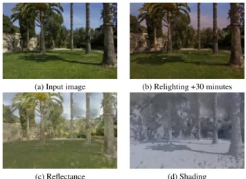
(a) Input image (b) Relighting +30 minutes

(c) Reflectance (d) Shading

Fig. 1: Our algorithm enables relighting with moving cast shadows from multi-view datasets (a,b). To do so, we separate each image into its re-flectance and shading components (c,d).

Each photograph in a multi-view dataset results from complex interactions between geometry, lighting and materials in the scene. Decomposing such images into intrinsic layers (i.e., reflectance and shading), is a hard, ill-posed problem since we have incomplete and inaccurate geometry, and lighting and materials are unknown. Pre-vious solutions achieve impressive results for many specific sub-problems, but are not necessarily adapted to automated treatment of multi-view datasets reconstructed with multi-view stereo, espe-cially in the presence of cast shadows. For example, previous in-trinsic image approaches can require manual intervention, special

hardware for capture, or restricting assumptions on colored light-ing; recent learning-based shadow detectors may not always pro-vide consistently accurate results, and previous inverse rendering methods require pixel-accurate geometry which cannot be auto-matically created using multi-view stereo. Our datasets can have 30-100 photographs allowing image-based navigation over a suffi-cient distance for image-based-rendering applications. We thus aim for an automatic method that scales to multi-view datasets while producing consistent quality results over all views under outdoor lighting.

Our method takes the multi-view stereo 3D reconstruction as in-put; our algorithm is designed to handle the frequent inaccuracies and missing data of such models. The user then specifies the sun di-rection with two clicks, and we automatically estimate parameters of our image formation model to extract the required reflectance, shading and visibility information.

The first key idea of our approach is to progressively improve the accuracy of the image model parameters with iterative estimation steps, by combining 3D lighting simulation with 2D image opti-mization.

Our second key idea is to use the image formation model to ex-press reflectance as a function of discrete visibility values – 0 for shadow and 1 for light – allowing us to introduce a robust visibility classifier for pairs of points in a scene.

Our method starts by finding a first estimate of sun and envi-ronment lighting parameters, as well as visibility to the sun. We then find image regions in shadow and in light, implicitly grouping regions of same reflectance. One significant difficulty of outdoors scenes is that they contain complex cast shadow boundaries. It is thus imperative to extract such boundaries as accurately as pos-sible, which we achieve by labeling shadows using our visibility classifier.

We present two main contributions:

—A method that combines multiple images and coarse 3D informa-tion to estimate a lighting model of the scene, including incident indirect and sky illumination as well as the color of sunlight. Inspired by the single-image method of [Lalonde et al. 2009; 2011], we first use the input images to automatically synthesize an approximate environment map. We then use the 3D informa-tion to perform lighting simulainforma-tion and deduce the unknown sun-light color.

—A method to compute multi-view intrinsic layers using shadow labelling and propagation. We use our robust visibility classifier in a graph labelling algorithm to assign light/shadow labels to all pixels except those in penumbra. We complete the computed intrinsic layers by propagating visibility to the remaining pixels in each image. The shadow classification is then used to improve the estimate of environment lighting, resulting in more accurate shading, visibility and reflectance layers.

Our automatic multi-view intrinsic decompositions provide high-quality layers of reflectance and shading. The high-quality of these de-compositions is sufficient to allow us to introduce a novel appli-cation, namely multi-view relighting with moving cast shadows. We do this by using the intrinsic layers and creating shadow-caster geometry which preserves shadow boundaries even when the 3D model is inaccurately reconstructed. We demonstrate our approach on several multi-view datasets, and show how it can be used to achieve IBR with illumination conditions different from those of the input photos.

2. RELATED WORK

Our work is related to inverse rendering and relighting, intrinsic images and shadow detection; in the interest of brevity we restrict our discussion to recent work most closely related to ours, and cite surveys where possible.

Inverse rendering and Relighting.A comprehensive survey of inverse rendering methods can be found in [Jacobs and Loscos 2006]. Early work [Yu and Malik 1998; Yu et al. 1999; Loscos et al. 1999] required geometry which was of sufficient quality for pixel-accurate cast shadows; this is also true for more recent work [Debevec et al. 2004; Troccoli and Allen 2008]. The geometry was either manually constructed, or scanned with often specialized equipment; similarly involved processes are also used to capture re-flectance. In contrast we target the often imprecise and incomplete 3D geometry reconstructed from casual photographs by automatic algorithms.

Karsch et al. [2011] generate plausible renderings of virtual ob-jects in photographs by performing inverse rendering from coarse hand-made geometry and a single image. Xing et al. [2013] pro-pose a similar single-image approach that also accounts for envi-ronment lighting in outdoor scenes. The manual steps and required geometry precision for cast shadow removal make these approaches unsuitable for relighting of multi-view datasets. Similarly, Okabe [Okabe et al. 2006] describes a user-assisted approach to recover normals from a single image and relight it. While the normals pro-vide enough information to compute local shading, cast shadows are not considered.

Photo collections have been used for relighting in [Haber et al. 2009] and [Shan et al. 2013]. These approaches require pictures taken under different lighting conditions while our goal is to al-low a user to capture a scene once with a single lighting condi-tion, and permit relighting. In particular, while the image formation model of Shan et al. [2013] is similar to ours, their algorithm lever-ages cloudy pictures to bootstrap reflectance estimation and tends to bake shadows in reflectance in the absence of sufficient light-ing variations. The method of Shih et al. [2013] performs lightlight-ing transfer by matching a single image to a large database of time-lapses, but cannot treat cast shadows.

Intrinsic images. An alternative to the accurate reflectance model estimation used in inverse rendering is image decomposi-tion into intrinsic layers [Barrow and Tenenbaum 1978], typically shading and diffuse albedo (or reflectance). The recent technical report of Barron and Malik [2013a] provides a good review of in-trinsic image methods. Automatic single image methods rely on as-sumptions or classifiers on the statistics of reflectance and shading [Land and McCann 1971; Shen and Yeo 2011; Zhao et al. 2012; Bell et al. 2014]. In particular, most methods assume a sparse or piece-wise constant reflectance and smooth grey illumination – the so-called Retinex assumptions. Closer to our work is the method of Garces et al. [2012] who group pixels of similar chrominance to form clusters that are encouraged to share the same reflectance. Ye et al. [2014] extend the method of Zhao et al. [2012] to videos by enforcing temporal coherence. These methods work well on single objects captured in a controlled setup [Grosse et al. 2009] but tend to fail on outdoor scenes where – as noted by [Laffont et al. 2013] – sun, sky and indirect illumination produce a mixture of colored lighting and produce cast shadows. Our method properly handles such cases by explicitly modeling the influence of sky and indirect illumination and by detecting shadow areas.

User-assisted methods [Bousseau et al. 2009; Shen et al. 2011] can handle colored shading but would be cumbersome for the multi-view image sets we target. Recent work has concentrated on

multi-image datasets requiring images with multiple lighting con-ditions, typically from photo-collections [Liu et al. 2008; Laffont et al. 2012]. Similar to inverse rendering methods, the need for mul-tiple lighting conditions makes their usage more complex for the casual capture context we target. This is also true of intrinsic image methods from timelapse sequences (e.g., [Weiss 2001; Sunkavalli et al. 2007].)

A second class of methods use either multiple images or depth acquired either from sensors or reconstruction. Some of these work on a single image e.g., [Lee et al. 2012; Barron and Malik 2013b; Chen and Koltun 2013]. While they improve over previous work, they may sometimes have difficulty removing cast shadows (see comparisons in Sec. 9.5). The work of [Laffont et al. 2013] is clos-est to ours, but requires special equipment (chrome ball, grey card) and manual selection of parameters. From an algorithmic stand-point, a major difference is that Laffont et al. treat sun visibility as a continuous variable, while we introduce a binary classifier of shadow regions. We found that explicitly estimating binary visi-bility improves robustness as it prevents this term to absorb errors from other shading terms in a non-physical way. Comparisons to [Laffont et al. 2013] and other methods in Sec. 9.6 show that our approach generally improves the quality of the decompositions.

Shadow detection.Shadow detection and removal have been studied extensively [Sanin et al. 2012] and most methods take a single image as input. Early approaches include automatic meth-ods (e.g., [Finlayson et al. 2004]) which were demonstrated on im-ages of uncluttered scenes with isolated shadows. More recent au-tomated approaches include [Lalonde et al. 2010; Zhu et al. 2010; Panagopoulos et al. 2013; Guo et al. 2012]. Similarly to these methods, our shadow estimation step (Sect. 6) identifies pairs of lit and shadow points sharing the same reflectance. However, ex-isting work detects such pairs using machine learning [Guo et al. 2012] or by approximating shading and reflectance with brightness and hue [Panagopoulos et al. 2013]. In contrast, we rely on mul-tiple images to estimate an environment map and an approximate 3D geometry, which we use to explicitly compute sun, sky and in-direct lighting. This additional information provides us with more accurate estimation of reflectance values between pairs of points, which in turn yields more robust shadow classification. Note also that the shadow classifier described in [Panagopoulos et al. 2013] is designed to provide a rough cue of sun visibility suitable for geom-etry inference, while we aim for finer shadow boundaries to remove the shadows from the image. Other methods [Wu et al. 2007; Shor and Lischinski 2008] require user assistance for each image which would be impractical for the multi-view datasets we target. We pro-vide comparisons in Sec. 9.5.

3. IMAGE MODEL AND ALGORITHM OVERVIEW

The image model we use is central to our method, since it clearly defines the quantities that need to be estimated. The model will also be used to guide the definition of our iterative process to estimate our multi-view intrinsic decomposition.

3.1 Image Model

We use the following image formation model [Laffont et al. 2013]: I = R ( vsunLsun cos(ωsun) + Ssky+ Sind), (1)

Iis the observed radiance (i.e., pixel value), R is the diffuse re-flectance of the corresponding 3D point, Lsunis the radiance of the

sun, vsunis the sun visibility from the point, ωsunis the angle

be-tween the normal n and the direction θsun to the sun, Sskyis the

radiance of the visible portion of the sky integrated over the hemi-sphereΩ centered at n, and Sindis the indirect irradiance integrated

overΩ, but excluding the sky. For all cosines we take max(0, cos) in practice; all values are RGB except for the cosine. We implicitly assume that R is diffuse.

Using Eq. 1, we can also write reflectance R as a function of visibility:

R(vsun) =

I

(Sind+ Ssky+ vsunLsun cos(ωsun))

(2) In some cases it is convenient to group sky and indirect light-ing into a slight-ingle environment shadlight-ing term Senv and write

Ssun = Lsun cos(ωsun), giving a simpler expression:

I = R ( vsunSsun+ Senv) (3)

3.2 Input

Our input is a set of linearized raw 12-bit/channel photographs of the scene, captured from different viewpoints at the same time of day and with same exposure. We use Autodesk Recap360 (http://recap360.autodesk.com) for all 3D reconstructions, taking the vertices of the reconstructed mesh as a point cloud. The qual-ity of the meshes is quite high overall with some residual noise for buildings, but often very approximate for structures such as vege-tation etc. Such methods also have difficulty reconstructing silhou-ettes and fine structures. Alternative methods (e.g., structure from motion [Snavely et al. 2006] followed by reconstruction [Goesele et al. 2007; Furukawa and Ponce 2007; Pons et al. 2007]) provide similar quality. In what follows we use the term proxy to refer to this – typically incomplete and inaccurate – 3D model.

Our method requires the sun direction θsun. Automatic methods

[Panagopoulos et al. 2013] can be used, however, we prefer to use a simple manual step, which is performed just after reconstruction and guarantees high-quality results. To determine the direction of the sun, a colored version of the point cloud is presented to the user. Each point is assigned the median value of pixels in all im-ages in which this 3D point is visible. The user clicks on a point in shadow and the corresponding 3D point which casts it, allowing the sun direction to be estimated. This simple process is shown in the accompanying video.

3.3 Estimating image-model quantities.

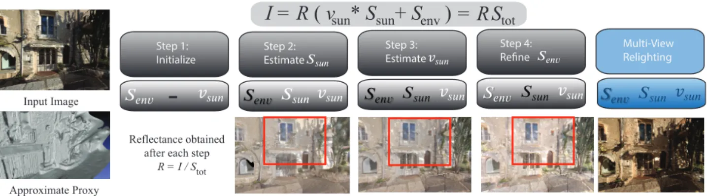
Our algorithm has four main steps, shown in Fig. 2. In each step we compute estimates of the quantities of Eq. 1, which are pro-gressively more accurate. To compute a reflectance layer R, we estimate shading Stot, and divide the input image to obtain R; this

is performed in Steps 2-4 and the result shown in Fig. 2. In con-trast with most previous work, our input contains strong cast shad-ows. Our goal is to obtain results of sufficient quality to perform re-lighting: this requires a reflectance layer free of shadow and other residues, as well a good estimate of shadow boundaries, environ-ment shading.

A guiding principle of our approach is that we prefer the explanation of a given scene that fa-vors a smaller number of reflectances, follow-ing previous work [Omer and Werman 2004; Barron and Malik 2013b; Laffont et al. 2013]. Consider the scene shown in the inset. There are two explanations for the dark areas on tablecloth: a shadow cast by the statue and plant or blobs painted in grey. Our approach favors the hypoth-esis with fewer reflectances, which explains the

Step 1: Initialize Step 2: Estimate Step 3: Estimate Step 4: Refine Input Image

I = R ( v *

S

+ S )

R = I / S tot tot

S

= R

Fig. 2: Our input are images (top left), an approximate 3D model (proxy) (lower left) and user-supplied sun direction. We use the image formation model (top) and estimate progressively better approximations to each of its parameters. In white, quantities estimated in a given step; quantities in black are fixed at that stage. Step 1: given the proxy we build a sky environment map and compute a first estimate of vsun

and Senvby ray-tracing the inaccurate 3D model and sky map. Step 2: we refine vsunand estimate Ssunusing luminance and chromaticity.

Step 3: given first estimates of all quantities we perform a graph labelling to further refine vsun. In Step 4 we refine Senv, and vsun in

penumbra, using the more accurate shadow boundaries now available. Reflectance is estimated at steps 2-4, and we clearly see how the result is progressively improved. Far right: during multi-view relighting, reflectance is fixed, and we can manipulate quantities in blue, resulting in a relit image (lower right; compare to top left).

image as a shadow over a uniformly white tablecloth. Throughout the four steps of our approach, we enforce this hypothesis by find-ing same-reflectance pairs between regions or points in light and shadow, inspired by previous work [Panagopoulos et al. 2013; Guo et al. 2011].

The key novelties of our approach are the automatic estimation of the parameters of Eq. 2, and the introduction of a robust shadow classifier using this information, see Sec. 6. Put together, these encourage the choice of the correct visibility configuration which finds same reflectance regions and implicitly connects (or merges) them via the pairs, thus enforcing the hypothesis.

The fours steps are illustrated in Fig. 2: In Step 1, we find initial values for Senv and vsun; in Step 2 we estimate Ssun, in Step 3

we obtain accurate shadow boundaries by refining the estimate of vsunand in Step 4 we refine the estimation of Senv. The estimated

reflectance improves significantly at each step.

Fig. 3: Left: the partial environment map. Right: completed synthesized environment map.

4. ESTIMATION OF SSKYAND SIND

To compute Sskyand Sind, we first automatically compute an

envi-ronment map to represent light coming from the sky and unrecon-structed surfaces1_{. We project all pixels of the input pictures that}

are not covered by the reconstructed geometry into this map. Fig. 3

1_{We described a preliminary version of the environment map computation}

in Chapter 4 of [Laffont 2012].

shows such a partial environment map where holes correspond to directions either not captured in the input photographs or directions corresponding to rays that intersect the proxy.

We apply a simple color-based sky detector to determine which pixels above the horizon in the map are sky and which are dis-tant objects. More involved approaches [Tao et al. 2009] could be used, but our approach sufficed in all our examples. The horizon is the main horizontal plane of the proxy. The visible portions of the sky give us strong indications on the atmospheric conditions at the time of capture. Inspired by Lalonde et al. [2009; 2011], we esti-mate the missing sky pixels by fitting the parametric sky model of Perez et al. [1993] from the partial environment map. This model expresses for any direction p the sky color relative to the color at zenith as a function of the angle θpbetween p and the zenith, the

angle γpbetween p and the sun direction, and the turbidity t that

varies with weather conditions [Preetham et al. 1999; Lalonde et al. 2009]. Since the color at zenith is itself an unknown, we need to re-cover a global per-channel scaling factor to obtain absolute values. We estimate the turbidity t of the sky model f and the scaling factor k by minimizing argmin t,k X p∈P (kf(θp, γp, t) − Ap) (4)

whereP denotes the set of known pixels in the environment map A. We solve this non-linear optimization with the simplex search algorithm (fminsearch in Matlab). At each iteration, the search algorithm generates a new value of the turbidity t that we use to update f , and then k from the new sky values by solving a linear system. We initialize the optimization by setting t = 3.5, which corresponds to the turbidity of a clear sky [Preetham et al. 1999]. We fill holes below the horizon line by diffusing color from nearby pixels.

Similarly to Laffont et al. [2013], we compute Sind and Ssky

by integrating the indirect and sky incoming radiance using ray-tracing. For each 3D point, we cast a set of rays over the hemisphere centered on the point normal. Rays that intersect the sky part of the environment map contribute to Ssky, while rays that intersect the ACM Transactions on Graphics, Vol. xx, No. x, Article xx, Publication date: xxx 2015.

proxy geometry or the non-sky pixels of the environment map con-tribute to Sind. We estimate the radiance coming from the proxy

geometry by gathering for each vertex the radiance in the images where this vertex appears. We assign the median of the gathered values as the approximate diffuse radiance of the vertex. Given the low frequency nature of these quantities, our approximations are generally sufficient. However, the non-diffuse nature of real sur-faces and errors in reconstruction can result in overestimation of indirect light. We thus introduce an approximate attenuation fac-tor which compensates for such errors by scaling with the cosine of the normal of the contributing surface when gathering at each point. Details of the implementation are given in the supplemental material.

The ray-tracing step also provides approximate visibilityv˜ to-wards the sun at each point, with respect to the proxy. The bound-aries defined by˜vcan be quite approximate however, as shown in Fig. 4(b). We improve the estimate of vsunin Step 3 (Sec. 6).

5. ESTIMATION OF SUN COLOR LSUN

Now that we have computed illumination from the sky and indirect transfer at all 3D points, we can estimate Lsunusing Eq. 1 and a

pair of points with same reflectance and different visibility. Given two points p1and p2with the same reflectance, with one in shadow

and the other in light, we can compute Lsun:

Lsun=

I1∗ (Ssky2+ Sind2) − I2∗ (Ssky1+ Sind1)

I2∗ vsun1∗ cos(ω1) − I1∗ vsun2∗ cos(ω2)

(5) All quantities for sun, sky and indirect are denoted with appropriate subscripts.

The main difficulty in using this formulation is that we do not yet have accurate reflectance and visibility necessary to find a suitable pair of points. While single-image intrinsic decomposition methods could be used to initialize the reflectance, most existing algorithms are challenged by outdoor scenes with hard shadows that break the Retinex assumptions of a smooth monochrome shading. We con-ducted preliminary experiments with the Retinex implementation of [Grosse et al. 2009], which confirmed that this algorithm does not remove hard shadows on our scenes. As a result, our calibra-tion algorithm was unable to find pairs of points sharing the same reflectance across shadow boundaries.

Instead of using Retinex, we found it sufficient at this stage to approximate reflectance with the image chrominance and shading with luminance, which we combine with the proxy-based visibility ˜

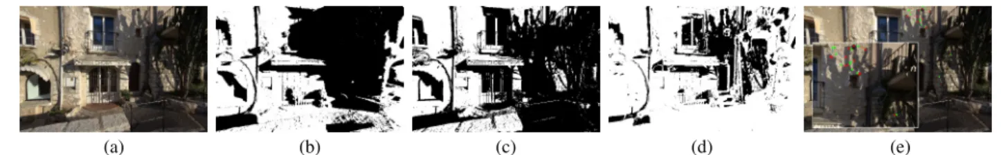
vfor a conservative estimate of shadow regions. More precisely, we first perform a K-means clustering on luminance. We found that im-age histograms typically contain two “extreme” clusters (dark and light, most often corresponding to shadow and light); to better sep-arate intermediate values two additional clusters are required. We thus used K= 4 in our implementation. For each cluster we com-pute the ratio of the number of points inside the proxy shadowv˜ to the number of points outside. We classify a cluster in shadow if its ratio is lower than the average ratio in the image. We then inter-sect the value ofv˜(Fig. 4(b)) with the classification of each pixel (Fig. 4(c)), resulting in very confident regions of shadow albeit cov-ering only a limited number of pixels in the image Fig. 4(d). Given this visibility estimate, we sample the shadow boundary regularly and for each sample we detect a lit (resp. shadowed) point away from the penumbra by walking in the two directions perpendicular to the boundary and selecting the pixel with the highest (resp. low-est) luminance and a similar chrominance. In our implementation we stop the walk after30 pixels in each direction and reject the samples for which no pixels with similar chrominance are found.

We also reject the sample if we cross a depth or normal discontinu-ity along the walk, identified with a Canny filter over the depth and normal map rendered from the proxy. Despite the inaccuracies of the proxy, in our tests only15% of the selected pairs did not share the same reflectance, or did not cross a shadow boundary. Taken over the entire view dataset, the selected pairs provide multi-ple estimators for Lsun, using Eq. 5 (Fig. 4(e)). We finally compute

a robust estimate of Lsunas the median of the solutions given by

all pairs.

We found that performing the median filter in each RGB channel separately gives the best results. This sparse set of pairs is approx-imate but sufficient for the calibration task. The later estimation of more accurate visibility boundaries will allow us to find a more reliable and denser set of light/shadow pairs and thus refine the es-timate of environment lighting.

At this stage, we have an estimate of all quantities of Eq. 1, namely ωsun, Ssky, Sindand Lsun; the estimate of vsun ≈ ˜v

how-ever is approximate. If we compute reflectance at each 3D point, we obtain approximate results that can have large regions of error (see leftmost image in Fig. 2).

6. ESTIMATING ACCURATE CAST SHADOWS AND INTRINSIC LAYERS

To compute residue-free reflectance layers for each image, we need to refine the accuracy of shadow boundaries and thus vsun. We

do this using a graph labeling approach, giving a binary label of shadow or light to all pixels, except those in penumbra. We assign a continuous visibility label to penumbra separately using matting (Sec. 6.2).

6.1 Shadow Labeling

The intuition behind our approach is to find the set of visibility la-bels that make most points share a similar reflectance, as explained earlier (Sec. 3.3). Consider two points s and t with visibility i and j respectively. Using Eq. 2 we compute the difference between their reflectances as:

Dij = |Rs(i) − Rt(j)|. (6)

Since i, j∈ {0, 1} we obtain four possible values of Dij. A small

value provides us with a strong evidence that s and t share the same reflectance under the corresponding visibility hypothesis. We illus-trate this sillus-trategy with the following toy examples:

Input

R

S

tot

D₀₁ low

D₀₀ medium D₁₀ high D₁₁ medium

s

t

The diagram below shows the case where s is in shadow and t is in light, both on a patch of roughly constant reflectance. Con-sider the case in the second column, which is the correct config-uration: the two points receive a similar reflectance, which makes D01 small. In contrast, D10is large, since the incorrect visibility

assumptions “pull apart” Rs(1) from Rt(0); see Eq. 2. The two

points also receive different reflectances when assigned the same visibility, i.e. D00and D11are larger than D01, although smaller

than D10. We can thus concentrate on comparing D10 and D01;

this provides a robust indicator of the correct visibility labels for

(a) (b) (c) (d) (e)

Fig. 4: The consecutive steps of the algorithm to determine Lsun for the “Street” scene. (a) Input image (b) shadow from inaccurate 3D

model: the proxy overestimates the geometry of the cactus and creates a “blob” shadow (c) K-means intensity estimation: some black areas are not shadows (d) intersection of (b) and (c): a more reliable subset of shadows are found, which are used in (e) to find pairs used to calibrate the sun.

the pair, under the assumption that the two points share a similar reflectance. Importantly, this information is directional, i.e., if s is in shadow, then we have a strong indication that t is in light.

D₀₁ medium

D₀₀ low D₁₀ medium D₁₁ low Input R S tot

s

t

The second diagram above shows a configuration where s and t have the same label (both in light in this case; both in shadow can be treated symmetrically), also with the same reflectance. Here we can distinguish clearly between same label cases (D00and D11) which

give a similar reflectance to s and t compared to the different-label cases. However, we cannot distinguish between the light/light or shadow/shadow case since they both make the two points have a similar reflectance. Pairs of points sharing the same visibility are thus somewhat less informative than pairs of points with different visibility. Both cases however provide reliable information which we use for shadow classification. Finally, points having different reflectances result in high Dijunder all four labeling

configura-tions.

We next define an energy that is minimized by the label con-figuration best explaining the same reflectance hypotheses. Specif-ically, we detect the pairs of points likely to have the same re-flectance and different visibility and use this directional informa-tion to initialize the labels at a few confident points (Fig. 5(a)). We then connect these points to their immediate neighbors and to other points with same reflectance and visibility, which allows us to propagate the labeling over the entire image (Fig. 5(b)). We ex-press this approach as a Markov Random Field (MRF) problem over a graph [Szeliski 2010; Kolmogorov 2006], where each node corresponds to a point s with label xs∈ {0, 1} and each edge (s, t)

connects a point s to another point t. NotingX the set of all labels xiof all nodes, we have

argmin X X s∈V φs(xs) + X (s,t)∈E φs,t(xs, xt), xi∈ {0, 1}. (7)

V denotes the set of nodes,E is the set of edges, φs(xs) is the

unary potential deduced from points with same reflectance and dif-ferent visibility, and φs,t is the pairwise potential that favors the

propagation of the labels. We detail the computation of the unary and pairwise potentials later in this section.

To solve this optimization, we could naively connect all pixels to all others, and perform the minimization on the resulting graph.

(a) Initialization (b) Final labeling

Fig. 5: (a) Initial labels from unary term, white is in light, black in shadow and grey undefined. (b) Final labels after convergence.

This is both inefficient and numerically unstable. We thus apply mean-shift clustering [Comaniciu and Meer 2002] in(L, a, b, x, y) space to segment the image into small regions where we can safely assume uniform reflectance and visibility, simplifying the problem and reducing noise (see Fig. 6). We use bandwidth parameters of 5 in space and 1 in color and a minimum region area of 50 pix-els, which results in around 6000 clusters for an image of size 1000 × 700 pixels. The values for R(0) and R(1) for a cluster are computed as the median values for all 3D points projected onto the cluster, except for points in a 3-pixel wide boundary around each cluster.

We solve our problem using a publicly available implementation of [Kolmogorov 2006]2_{. The potentials take values l}

1 = 1,

l0 = 0 when strongly encouraging one hypothesis over the other,

lp = 0.8, lnp = 0.2 for the case when one hypothesis is

mod-erately preferred over another (“non-preferred”) and leq = 0.5

when both hypothesis are equally encouraged.

Unary Potential.As many binary labeling problems, a good ini-tialization is central to obtain a good solution. Given the discussion above, we use pairs of clusters likely to have the same reflectance and different visibility to initialize our unary term. In particular, for a cluster s we find the setS of k other clusters with the smallest D01 and the setL of k other clusters with the smallest D10. The

clusters inS favor the hypothesis that s is in shadow, while the clusters inL consider that s is in light. We compute the score of each hypothesis as the sum of the reflectance differences between

2

http://research.microsoft.com/en-us/downloads/dad6c31e-2c04-471f-b724-ded18bf70fe3/ ACM Transactions on Graphics, Vol. xx, No. x, Article xx, Publication date: xxx 2015.

(a) Input (b) Meanshift clustering (c) Cluster boundaries

Fig. 6: We apply meanshift clustering to decompose the image in small regions of uniform color. We then solve the shadow labeling on a graph of clusters rather than pixels, which reduces the number of unknowns and the impact of noise.

sand the k other clusters H0 = X t∈S |Rs(0) − Rt(1)| (8) H1 = X t∈L |Rs(1) − Rt(0)| (9)

where Rs(i) and Rt(i) are computed with Eq. 2.

If H0

H1+ H0 < τ1, i.e., the hypothesis that s is in shadow is

stronger, we set the unary potential to prefer the “in shadow” la-bel: φs(xs) = ( l0 for xs = 1 l1 for xs = 0 (10) Conversely, if H1

H1+ H0 < τ1, we set the unary potential to prefer

the label “in light”: φs(xs) =

(

l1 for xs = 1

l0 for xs = 0

(11) If neither condition is true we perform a more localized search. We compute two new hypothesis H′

1and H0′ in the same manner as

Eq. 8, but restrict the k clusters to lie within a neighborhood around s. We then check if:

H1 + H1′

H0 + H1 + H0′ + H1′

< τ1 (12)

and similarly for the H0 hypothesis, which can be seen as a more

“permissive” hypothesis, since we complement the best global can-didates with the best local ones. If one of these conditions is met, we set the potentials the same way as above. If none of the condi-tions are met, the unary potentials are set to equally prefer either hypothesis:

φs(xs) = leq, xs∈ {0, 1} (13)

We used τ1 = 0.1, corresponding to a 90% confidence level

re-quired to make a decision.

Pairwise Interaction Potentials.The goal of our pairwise po-tentials is to propagate labels between clusters with the same visi-bility. We first create edges between each cluster s and other clus-ters with similar reflectance, which we select as the k clusclus-ters with smallest D00or D11. For these edges, the values of the potentials

are set to strongly encourage the same label to be propagated: φs,t(xs, xt) =

(

l1 when xs = xt

l0 when xs 6= xt

(14)

However, these edges alone are not always sufficient to ensure that the graph forms a single connected component. We prevent iso-lated components by also connecting each cluster with its immedi-ate neighbors. In the absence of other cues, we define the potential of these weaker connections to encourage clusters with the same color distribution to share the same visibility. We compute the χ2

histogram distance dcin Lab space for clusters s and t using the

approach described in [Chaurasia et al. 2013]. Clusters s and t are similar for dc < τc; in this case we assume they most probably

have the same label: φs,t(xs, xt) =

(

lnp when xs = xt

lp when xs 6= xt

(15) If the χ2 _{distance is too large however, all potentials are set to}

equally prefer all possible hypotheses.

φs,t(xs, xt) = leq, xs, xt∈ {0, 1} (16)

We used τc = 0.05 for all our tests, which corresponds to the

acceptance probability in the χ2_test.

At convergence, we obtain accurate shadow boundaries, even though there can be some occasional miss-classifications, e.g., the letters on the store front in Fig. 5(b). Such errors typically occur in small regions that contain few or no 3D points. In the former case, the median reflectance candidates R(0) and R(1) are more likely to be polluted by occasional reprojection errors and specu-larities, while in the latter case the propagation is solely governed by the χ2_{distance to neighboring regions. Nevertheless, erroneous}

regions tend to be small in size, and thus do not affect the applica-tion to relighting.

6.2 Per-pixel Estimation of vsunand Intrinsic Layers

The binary labeling cannot capture soft shadows. We apply Lapla-cian matting [Levin et al. 2008] to recover continuous variations of visibility in the boundaries between clusters. These correspond to penumbra regions at the frontier of shadow and light clusters, effec-tively providing a tri-map from the binary shadow mask. We also apply Laplacian matting guided by the input image to propagate the shading values Ssky, Sindand Ssun, as previously done by Laffont

et al. [2012]. We use all 3D points except those in the boundaries between clusters as constraints in this propagation. While these smooth shading layers do not contain shadows, propagating them using the input image as guidance sometimes produces artifacts along shadow boundaries. We reduce these artifacts by excluding a small band along shadow boundaries from the propagation, which we subsequently fill with a color diffusion. The reflectance layer is obtained by dividing the input image by the sum, or total shading Stot

Stot = Ssky + Sind + vsunSsun. (17)

The classifier can occasionally miss very fine shadow structures which are however captured by the clusters; we also propagate vis-ibility in the boundary regions between clusters, which generally improves the visual quality for relighting (see Sec. 9.9).

7. REFINING ENVIRONMENT SHADING AND REFLECTANCE ESTIMATION

The quality of the intrinsic layers obtained so far is limited by the accuracy of the different radiometric quantities computed. In par-ticular, the success of using Eq. 2 to compute R is dependent on the approximations in our estimations of Senv, Lsunand vsun. As ACM Transactions on Graphics, Vol. xx, No. x, Article xx, Publication date: xxx 2015.

(a) Reflectance before correction

(b) Same-reflectance pairs across shadow boundary

(c) Reflectance after correction

Fig. 7: (a) The reflectance is discontinuous across the shadow boundary due to incorrect estimation of shading. (b) Pairs chosen as constraints to impose the same reflectance on both sides of the boundaries. (c) Corrected reflectance after optimization.

we see in Fig. 7(a), the currently estimated values leave a visi-ble residue in the reflectance layer, which should be continuous (Fig. 7(c)). This discontinuity occurs because the values of Senv

and Lsun were computed using the incomplete and inaccurate 3D

reconstruction, and are thus approximate.

0 1 0 1 0 1 0 1 0 1 0 1 0 1 Input image I Ssun Senv R = I / (S_sun + S_env ) xsl R_s R_l Ssun Sn env incorrect values refined values Rn _{= I / (S} sun + S n env )

Fig. 8: 1D visualization of Senvrefinement. Small errors in our estimates of

L_sunand Senvcan prevent the reflectance to be continuous across shadow

boundaries (middle). We detect pairs of points with similar reflectance on each side of the boundary (orange dots) and compute a local offset of Senv

(blue) that makes the two reflectances equal (right).

We illustrate this in Fig. 8 where we show a plot of image inten-sity across a shadow boundary, with the shadow region on the left. In the middle column, we see the decomposition of the image into reflectance (Rsin shadow and Rlin light), and shading, composed

of Ssunand Senv. We will refine the value of shading so that Rs

becomes equal to Rl, by adding an offset to Senv. We correct Senv

since it is a continuous quantity over the shadow boundary. Specif-ically we apply an offset xslto Senv on both sides of the shadow

boundary so that Rsbecomes equal to Rl(Fig. 8, right).

We first find a dense set of same reflectance light/shadow pixel pairs along the shadow boundaries, Fig. 7(b). For each pair, we compute an offset xslwhich makes the two reflectances equal. We

then smoothly propagate the offsets to all pixels while preserving the variations of Senv, yielding the refined layer Senvn , Fig. 7(c).

The values of vsunin penumbra were determined by image-driven

propagation, which can sometimes result in high-frequency inac-curacies of vsun. These cannot be captured by the smooth

propa-gation, and we thus treat these pixels separately by correcting the vsunlayer.

Implementation details of the above steps for Senv refinement

are described in the supplemental material.

8. APPLICATION: MULTI-VIEW RELIGHTING WITH MOVING CAST SHADOWS

The automatic nature of the process and the high quality of the in-trinsic layers for reflectance R, shading Ssun, Senv and visibility

vsunallow us to introduce the novel application of multi-view

re-lighting.

Creating Shadow Receiver and Caster Geometry.Recall that shadows cast from the proxy are not accurate enough for relighting, since they do not correspond well to shadow boundaries in the im-age (see Fig. 4(b)). We approximate moving cast shadows by creat-ing a geometric representation of a caster from the shadows in the original image. While creating caster geometry is related to shape-from-shadow techniques [Savarese et al. 2007], such methods re-quire shadows from multiple light sources. In our case, we only have shadows from a single position of the sun. We thus design an approximate algorithm that (a) preserves the original shadow boundaries in the input image as much as possible and (b) allows some motion of the sun.

We first reconstruct the receiver geometry by assigning to each pixel the depth value of the closest projected 3D point. We found that the resulting depth map, while approximate, results in plausible shadows that we can composite over the reflectance image. We then estimate the geometry of the caster such that it produces shadows that match the shadow boundaries in the original images. We iden-tify the shadow boundaries from the shadow classification layer (e.g., Fig. 5, right) as well as from the propagated vsunlayer that

sometimes capture fine details lost by the binary classifier (Fig. 21, Sec. 9.9). We consider pixels to be in shadow if pixel p is classified as shadow in the former, or if vsun(p) < τs. We used τs = 0.8

for all our results. To estimate a 3D caster position at each shadow pixel, we shoot rays in the direction of the sun θsunand record the

distance of the closest intersection with the 3D proxy. Pixels for which the ray does not intersect the proxy receive the distance of the nearest valid pixel. We triangulate the shadow pixels in image space to create a mesh that we lift in the direction of the sun using the recorded distance. Fig. 9 illustrates the resulting 2.5D caster which re-creates the shadow boundary in the image.

Incorrect reconstruction and numerical imprecision can result in erroneous triangles that partly re-project on lit pixels. We remove such triangles by visiting all pixels in light and casting rays in the sun direction. If a triangle of the caster mesh is intersected by more than ǫ such rays, it is removed. We used ǫ = 3 for all our re-sults. Our shadow labeling also sometimes mis-classifies pixels as shadow in small regions. To filter these errors we cluster the pix-els in shadow and remove small clusters (less than 100 pixpix-els) and clusters for which less than30% of the pixels yield and intersection with the proxy. We adjust the reflectance of such pixels to bring them in light using the vsunlayer.

Moving Shadows and Adjusting Shading.To move shadows, we simply change the sun direction θsun and cast rays from each

pixel in that direction. We compute intersections against the caster using the Intel embree library, which provides interactive feedback for the images shown here (see also the accompanying video). Our caster geometry only reproduces the shadows captured in the im-age. As a result, discontinuities can appear when the shadow move away from the border. We complete the missing shadow in these areas using the shadow of the proxy geometry. Finally we apply a

Fig. 9: Left: Input image. Middle: detected shadow pixels in blue, shadow from the proxy in dark blue. Right: The caster mesh generated from these shadow pixels.

small Gaussian blur on the new shadow layer to mimic soft shad-ows and to fill small holes caused by disconnected triangles in the caster mesh.

We render an approximate effect of illumination changes by ad-justing the sun shading intensity according to a cosine factor with respect to elevation and the horizontal plane, and shifting Ssky

to-wards red in the morning and afternoon. We also diminish Sind

with a similar amount to maintain the illusion of shading change. Finally, we detect sky pixels and change their color near the hori-zon.

9. RESULTS AND COMPARISONS

We first present results of our decomposition algorithm for a num-ber of real-world scenes, as well as application to relighting. We then provide five evaluations of our method: 1) A ground-truth quantitative evaluation of our algorithm and comparison to [Laf-font et al. 2013]; 2) A ground-truth comparison of our synthetic relighting with real photographs taken at different times. 3) A vi-sual comparison of our algorithm with state-of-the art intrinsic im-age methods and shadow classifiers; 4) A comparison of our au-tomatic sunlight calibration and environment map estimation with the method of Laffont et al. [2013], which uses a grey card and chrome ball; 5) An evaluation of the robustness of our approach to decreasing number of input images.

In supplemental material, floating point versions of all layers of our decompositions are provided; however, different tone mapping had to be applied to each image to allow visibility of the results in this document.

9.1 Intrinsic Decomposition Results

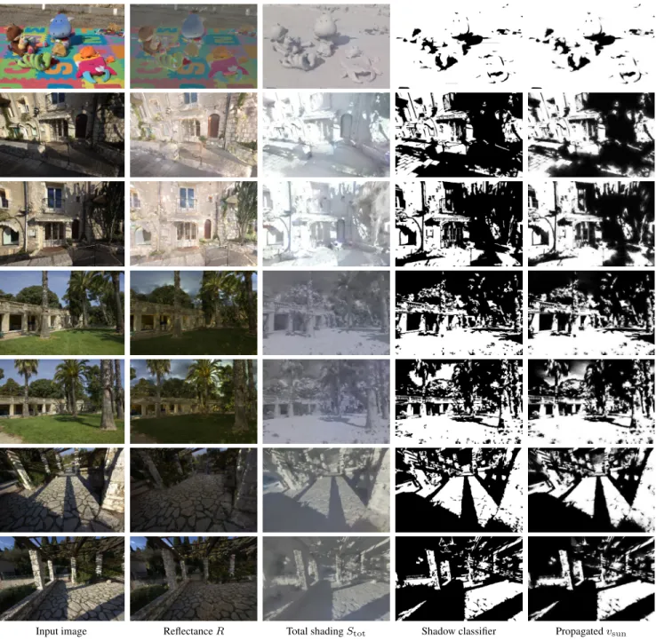
We present results on a variety of scenes. We show two test scenes with a small number of objects (Plant, Fig. 16) and Toys (Fig. 10, top row). We also show three natural scenes with buildings, veg-etation and thin structures (Fig. 10). In most cases we obtain re-flectance layers with little shadow and lighting residue, which are thus suitable for relighting. The shadow classifier and visibility lay-ers are also of high quality overall; occasional miss-classifications are usually in small regions, which can be detected and be removed when moving the shadows for relighting. The strongest errors occur in scenes with poor geometric reconstruction, as is the case in the second and third row of Fig. 10 where large portions of the tree as

well as the small wall in front of the scene are missing. Such holes in the geometry affect all the steps of our algorithm, from the com-putation of indirect lighting to the initialization of shadow regions and sun calibration. As a result, our shadow classifier has moder-ate success in identifying the shadow over the ground. Finally, the ground is dominated by variations of grey reflectance, which adds to the difficulty of shadow detection as some of these variations are well explained as shadows. The results for all views in each datasets are provided as supplemental material.

9.2 Relighting and Image-Based Rendering

We show results for relighting of the Villa scene in Fig. 1 and Fig. 12, for Street in Fig. 2, for Monastery in Fig. 11 and for Plant in Fig. 15. We performed relighting of up to 2 hours away from the time of capture, after which the shadow starts to break apart (Fig. 12). The maximum time variation that our method can achieve depends on the complexity of the shadow caster and the quality of its 3D reconstruction.

Our relighting approach can be used for image-based rendering (IBR) and changing lighting conditions. In the accompanying video we show an IBR view interpolation and free-viewpoint navigation path in the Villa dataset in which we use the algorithm of [Chaura-sia et al. 2013]. We record the path, change lighting conditions and play it back with the new illumination, since all the input images used for IBR have been updated.

Our method (Initial position) Using proxy (Initial position)

Our method (1 hour motion) Using proxy (1 hour motion) Fig. 11: Synthetic relighting. Our method reproduces the initial image well (upper left), and maintains shadow detail during relighting (lower left). In contrast, the proxy shadow looses many fine details (right).

9.3 Ground Truth Decomposition Evaluation

We purchased a model of a scene which has a similar ap-pearance to the real environments we target, with realistic tex-tures for the building, densely foliaged trees and we used a physically-based sky model [Preetham et al. 1999]. We used an in-house path-tracer to render 44 images, which we took as in-put for our complete pipeline. We also rendered the correspond-ing layers of reflectance and shadcorrespond-ing for quantitative comparison.

Input image Reflectance R Total shading Stot Shadow classifier Propagated vsun

Fig. 10: Our extracted layers on a variety of scenes: toys, urban (top), vegetation (middle), thin structures (bottom).

Multi-view stereo has difficulty with synthetic models and textures, and the quality of the reconstruction is poor, as can be seen in the inset; large portions of the tree are not well reconstructed and the overall geometry is coarse and approximate.

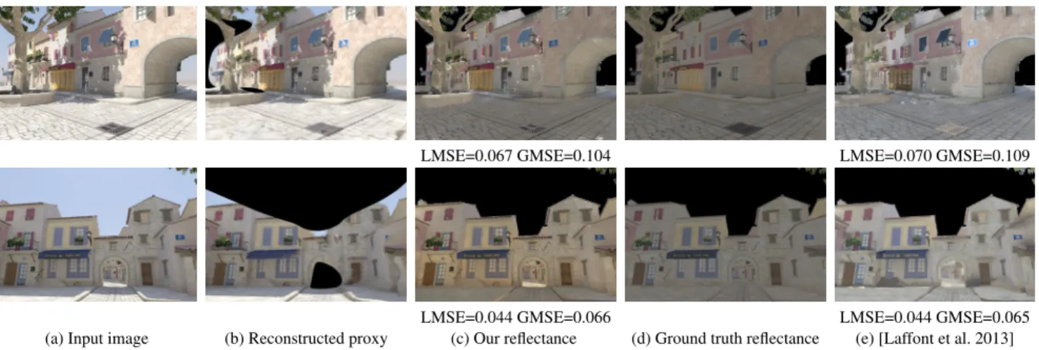
Figure 13 provides a visual and quantitative comparison of our reflectance against ground-truth and the result of Laffont et al. [2013]. We selected the parameters of [Laffont et al. 2013] that produce the best decomposition. The two methods yield results of

similar quality as measured by the LMSE and GMSE error met-ric [Grosse et al. 2009]. However, close inspection reveals that most of our error is due to mis-classification of small shadow re-gions, which yields strong yet localized deviation from ground-truth, while [Laffont et al. 2013] fails to completely remove the shadow of the tree on the wall, which yields a low yet extended er-roneous region (Fig. 13, top, far right). This different type of error is due to the fact that the method of Laffont et al. does not explic-itly estimate binary visibility and does not refine the estimation of environment shading; our approach yields results more suitable for relighting.

(a) - 2 hours (b) - 1 hour (c) Input image (d) + 1 hour (e) + 2 hours and 30 minutes

Fig. 12: Relit images for different times of day. While our method can produce drastic motions of the shadows (a-d), the shadow of the central tree breaks apart after a deviation of more than 2 hours (e).

LMSE=0.067 GMSE=0.104 LMSE=0.070 GMSE=0.109

LMSE=0.044 GMSE=0.066 LMSE=0.044 GMSE=0.065

(a) Input image (b) Reconstructed proxy (c) Our reflectance (d) Ground truth reflectance (e) [Laffont et al. 2013]

Fig. 13: Comparison between our method, [Laffont et al. 2013] and ground truth reflectance rendered from a synthetic scene. Our method produces a few strong yet localized errors due to mis-classification of small regions in the shadow of the tree. In contrast, [Laffont et al. 2013] exhibits a low yet extended deviation from ground truth in the shadow region. The two methods are quantitatively similar according to the LMSE and GMSE error metrics.

We provide additional comparisons on real-world scenes in Section 9.5. Figure 14 visualizes our error on reflectance and environment shading. This visualization reveals that a significant part of our er-ror is due to the approximate environment shading, especially in areas where this component dominates sun shading.

0.0316 0.0289 0.0224 0.0129 0.0183 MSE Error Reflectance 0.0949 0.0866 0.0671 0.0387 0.0548 MSE Error Environment

(a) Reflectance error (b) Senverror

Fig. 14: Visualization of MSE error for our reflectance (a) and refined envi-ronment shading Senv(b).

9.4 Ground Truth Relighting Evaluation

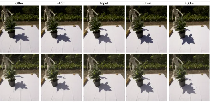
We captured several lighting conditions for the Plant scene to allow a ground truth comparison. We only used multi-view capture of the central image (i.e., a single lighting condition) for all intrinsic de-composition and relighting computations. We show the results in Fig. 15. We can see that the cast shadow becomes more approxi-mate as we move away from the time of capture used by our al-gorithm, but the overall appearance is plausible. A slight residue of the original penumbra remains visible in the reflectance, which is due to the non-diffuse nature of the white tablecloth we placed on the table. Since the camera is close to the glossy lobe of this surface, our assumption of diffuse reflectance reaches its limits and our refinement step is not sufficient to fully correct for the remain-ing errors. Note also that our synthetic shadows have the same color as the shadow in the input image because they are computed from an estimate of the same sun color and sky model. In reality the ap-pearance of the sky changed over time, which explains why the real shadow is darker in some pictures.

-30m -15m Input +15m +30m

Fig. 15: Above: real photographs taken at different times than those used for the algorithm. Below: relit images using our algorithm.

9.5 Comparisons with Intrinsic Image Algorithms

Our method takes as input multiple images and a 3D reconstruc-tion. For comparisons we focus on recent methods that also com-bine images and 3D information. Specifically we compare to two single-image methods based on RGB+depth data [Barron and Ma-lik 2013b; Chen and Koltun 2013] and the multi-view method of [Laffont et al. 2013]. From the results presented in these papers, these methods outperform single-image solutions that do not use depth, which are typically derived from the Retinex algorithm. We used the original code of these papers, and reported results to the authors who ensured that we set parameters correctly.

We present two test scenes for comparisons in Fig. 16 and the supplemental document. The first (“Plant”) is a simple scene, with a cast shadow on a tablecloth. The proxy reconstruction is of quite high quality except for the plant. From the results we can clearly see that the single image methods are not suited to outdoor scenes with cast shadows, and there is always a residue in the reflectance layer. Our algorithm benefits from the better 3D reconstruction provided by multi-view stereo. The method of [Laffont et al. 2013] also has some residue due to their use of approximate non-binary visibility values that tend to compensate for errors in the estimated shad-ing. By enforcing binary visibility we obtain robust shadow clas-sification, and consequently correcting reflectance across shadow boundaries in a reliable manner, our method produces better results overall.

Recall that, compared to [Laffont et al. 2013], all steps in our approach are automatic, removing the need for the chrome ball, grey card, parameter setting and inpainting steps. Figure 17 pro-vides a comparison between our automatic decomposition and a downgraded version of our algorithm where we used the captured chrome ball and grey card calibration of [Laffont et al. 2013]. Our calibration estimates a sun color of(2.7, 2.3, 2.4) while the grey card yields(2.7, 2.7, 2.7). Our estimated environment map cap-tures the overall color distribution of the sky and ground and results

Fig. 17: Comparison using a chrome ball and grey card (left) and our syn-thesized environment map with automatic calibration (right). Although our environment map misses details on the ground and horizon, it captures the overall color distribution of the ground and sky, yielding reflectance results (lower row) visually similar to the ones obtained with additional informa-tion.

in a reflectance on par with the one obtained with a chrome ball and manual calibration.

Floating point versions for all layers in the figures are provided as supplemental material. We also present additional comparisons for the Toys dataset, and we discuss the different tradeoffs between the artifacts in each approach.

9.6 Comparisons with Shadow Classifier Algorithms

Figure 18 shows a comparison with two single-image shadow clas-sifier methods [Zhu et al. 2010] and [Guo et al. 2011]. Our clasclas-sifier works well in most cases, and compares favorably to the previous approaches. The method of [Guo et al. 2011] often gives very good

Input image [Chen and Koltun 2013] [Barron and Malik 2013b] [Laffont et al. 2013] Our method

Fig. 16: Comparisons with existing intrinsic image methods, reflectance and shading respectively top and bottom row. Results are shown with scale factor and gamma-correction. Our approach removes the hard shadow, which allows us to subsequently relight the scene.

Input image [Zhu et al. 2010] [Guo et al. 2011] Our method

Fig. 18: Comparison with existing shadow classifiers. [Zhu et al. 2010] misses shadow details while [Guo et al. 2011] tends to produce false positives. Our approach leverages 3D information to avoid such errors.

results (last row), but can sometimes reports false positives or fails (top row).

9.7 Impact of Number of Input Images

Table I details the number of images used for each scene, along with the number of vertices of the proxy geometry. As is often the case

with multiview stereo reconstruction, we found it easier to capture a large number of images rather than attempting to find the smalest set of images that would be sufficient to run our method. In theory, lowering the number of input images can impact several aspects of our pipeline. First, using fewer images results in fewer sam-ples to estimate the diffuse radiance of the proxy geometry (Sec. 4)

Street Monastery Villa Statue Toys

#images 61 61 138 60 73

#proxy 2Mi 2.2Mi 6Mi 4.6Mi 4.6Mi

Table I. : Number of input images and number of vertices of the estimated 3D proxy, for each dataset.

Fig. 19: 3D reconstruction with 138, 68 and 34 views. The reconstruction is increasingly incomplete as we lower the number of images. See Fig. 20 for the corresponding intrinsic decompositions.

and fewer candidate pairs for sun calibration (Sec. 5). More impor-tantly, using fewer images yields a sparser 3D reconstruction which can miss significant parts of the geometry, lowering the quality of our initial estimation of visibility and indirect lighting. A sparser reconstruction also provides fewer point constraints for our shadow labelling algorithm (Sec. 6).

We conducted a small experiment to evaluate the practical impact of the number of input images on the quality of the end decomposition. Figure 20 shows that despite reducing the number of images from 138 to 34 our algorithm produces consistent results. This success is due to the fact that our shadow labeling algorithm leverages image information to identify accurate shadow regions even when the shadow caster is not well reconstructed, as shown in Figure 19.

9.8 Timings

The following table shows the average computation times on a 2.3Ghz E5-2630 PC for each step. Steps 1-3 are implemented in C++, with the exception of the optimization for the sky model which is in Matlab. The entry for Step 4 reports the time to solve the system using an unoptimized Matlab implementation.

Step 1. Init 2. Estimate Ssun* 3. Estimate vsun* 4. Refine Senv*

Time 5 min 1 min 3 min 3 min

Table II. : Average timings for each step. Step 1 is total timing for the entire dataset, while for Step 2-4 we report the timing per image marked by *.

9.9 Limitations

The quality of the initial reconstructed model affects all stages of our approach. Some geometry is required in the initialization step, most notably for the computation of Sindand Ssky, but also for the

Lsunestimation. If the geometry is completely incorrect, the initial

estimates will not be sufficient for the method to work.

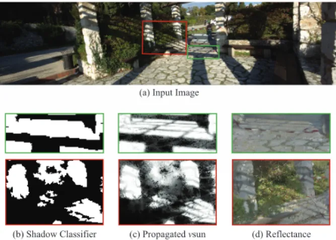
As mentioned previously, while the shadow classifier is overall very successful, it can occasionally miss-classify some regions, es-pecially for fine structures. The propagation of visibility in the clus-ters can correct some of these (green region in Fig. 21)). In other regions however, the reflectance will contain some residue (red re-gion in Fig. 21).

(a) Input Image

(b) Shadow Classifier (c) Propagated vsun (d) Reflectance

Fig. 21: Failure case: The fine structures (a few pixels wide) were not captured by the the classifier. In some cases the propagated visibility cor-rects these (green region), but in others the error remains as a residue in reflectance (red region).

10. CONCLUSION AND DISCUSSIONS

The method we presented is the first to allow automated intrin-sic image decomposition for multi-view datasets, providing re-flectance, shading and cast shadow layers at a quality level which is suitable for relighting. We are thus able to introduce multi-view relighting, and demonstrate its utility for IBR with changing illu-mination.

Our approach opens up many possibilities for future work. Cur-rently, our approach assumes outdoors scenes with sunlight and well-defined cast shadows. For scenes with overcast sky, the prob-lem is simpler, since the variation between shadow and light is much smoother. Precise determination of shadow boundaries is thus unnecessary. However, our approach must be extended to han-dle such soft boundaries, possibly with a new soft shadow classi-fier approach. We have shown our results using multi-view stereo, but other methods to acquire 3D data and images (e.g., Kinectfu-sion with RGB information [Nießner et al. 2013]) could be used in our algorithm with no significant changes. However, a single im-age with depth would probably not provide enough information to initialize Sskyand Sind, which are required to bootstrap our

pro-gressive estimation of reflectance, shading and shadows.

Another direction for future work is the development of a more complete image formation model that incorporates non-diffuse be-havior. This is an exciting fundamental research direction which requires a completely new approach to intrinsic image decomposi-tion.

Apart from IBR, other applications of multi-view relighting are possible, for example in compositing for post-production, where lighting changes often involve a significant amount of manual

Input images Reflectance with 138 views Reflectance with 68 views Reflectance with 34 views

Fig. 20: Decreasing the number of input images does not have a significant impact on the quality of the decomposition. See Fig. 19 for the corresponding 3D reconstruction.

work. In conclusion, by allowing multi-view relighting, our solu-tion takes an important step in making image-based methods a vi-able alternative for digital content creation.

Acknowledgements

We thank S. Paris for proof-reading the document and provid-ing valuable suggestions, R. Guerchouche for help in capture and preprocessing, L. Robert and E. Gallo for their support and help. This work was funded by an industrial collaboration between Inria and Autodesk. We acknowledge funding from the EU FP7, grant agreement 611089 - project CR-PLAY (www.cr-play.eu), and grant agreement 288914 - project VERVE (www.verveconsortium.eu).

REFERENCES

BARRON, J.ANDMALIK, J. 2013a. Shape, illumination, and reflectance from shading. Tech. rep., Berkeley Tech Report.

BARRON, J. T.ANDMALIK, J. 2013b. Intrinsic scene properties from a single RGB-D image. CVPR.

BARROW, H. G.AND TENENBAUM, J. M. 1978. Recovering intrinsic scene characteristics from images. Computer Vision Systems 3, 3–26. BELL, S., BALA, K.,ANDSNAVELY, N. 2014. Intrinsic images in the wild.

ACM Transactions on Graphics (Proc. SIGGRAPH) 33,4.

BOUSSEAU, A., PARIS, S.,ANDDURAND, F. 2009. User-assisted intrinsic images. ACM Trans. Graph. 28, 5, 1–10.

CHAURASIA, G., DUCHENE, S., SORKINE-HORNUNG, O.,ANDDRET -TAKIS, G. 2013. Depth synthesis and local warps for plausible image-based navigation. ACM Trans. on Graphics (TOG) 32, 3, 30:1–30:12. CHEN, Q.ANDKOLTUN, V. 2013. A simple model for intrinsic image

decomposition with depth cues. In ICCV. IEEE.

COMANICIU, D.ANDMEER, P. 2002. Mean shift: A robust approach toward feature space analysis. Pattern Analysis and Machine Intelligence,

IEEE Transactions on 24,5, 603–619.

DEBEVEC, P., TCHOU, C., GARDNER, A., HAWKINS, T., POULLIS, C., STUMPFEL, J., JONES, A., YUN, N., EINARSSON, P., LUNDGREN, T., FAJARDO, M.,ANDMARTINEZ, P. 2004. Estimating surface reflectance properties of a complex scene under captured natural illumination. Tech. rep., USC Institute for Creative Technologies.

FINLAYSON, G. D., DREW, M. S.,ANDLU, C. 2004. Intrinsic images by entropy minimization. In ECCV. 582–595.

FURUKAWA, Y.ANDPONCE, J. 2007. Accurate, dense, and robust multi-view stereopsis. In Proc. CVPR.

GARCES, E., MUNOZ, A., LOPEZ-MORENO, J.,ANDGUTIERREZ, D. 2012. Intrinsic images by clustering. Computer Graphics Forum (Proc.

EGSR) 31,4.

GOESELE, M., ACKERMANN, J., FUHRMANN, S., HAUBOLD, C.,AND KLOWSKY, R. 2010. Ambient point clouds for view interpolation. ACM

Transactions on Graphics (TOG) 29,4, 95.

GOESELE, M., SNAVELY, N., CURLESS, B., HOPPE, H., ANDSEITZ, S. M. 2007. Multi-view stereo for community photo collections. In

ICCV.

GROSSE, R., JOHNSON, M. K., ADELSON, E. H.,ANDFREEMAN, W. T. 2009. Ground-truth dataset and baseline evaluations for intrinsic image algorithms. In ICCV.

GUO, R., DAI, Q.,ANDHOIEM, D. 2011. Single-image shadow detection and removal using paired regions. In CVPR, 2011. IEEE, 2033–2040. GUO, R., DAI, Q.,ANDHOIEM, D. 2012. Paired regions for shadow

detec-tion and removal. IEEE Transacdetec-tions on Pattern Analysis and Machine

Intelligence 99.

HABER, T., FUCHS, C., BEKAER, P., SEIDEL, H.-P., GOESELE, M.,AND LENSCH, H. 2009. Relighting objects from image collections. In CVPR. 627–634.

JACOBS, K.ANDLOSCOS, C. 2006. Classification of illumination methods for mixed reality. In Computer Graphics Forum. Vol. 25. Wiley Online Library, 29–51.

KARSCH, K., HEDAU, V., FORSYTH, D.,ANDHOIEM, D. 2011. Ren-dering synthetic objects into legacy photographs. ACM Transactions on

Graphics (TOG) 30,6, 157.

KOLMOGOROV, V. 2006. Convergent tree-reweighted message passing for energy minimization. Pattern Analysis and Machine Intelligence, IEEE

Transactions on 28,10, 1568–1583.

LAFFONT, P.-Y. 2012. Intrinsic image decomposition from multiple pho-tographs. Ph.D. thesis, University of Nice Sophia-Antipolis.

LAFFONT, P.-Y., BOUSSEAU, A.,ANDDRETTAKIS, G. 2013. Rich intrin-sic image decomposition of outdoor scenes from multiple views. IEEE

Trans. on Visualization and Computer Graphics 19,2, 210–224. ACM Transactions on Graphics, Vol. xx, No. x, Article xx, Publication date: xxx 2015.