Distributed Throughput Maximization in Wireless Networks via Random Power Allocation

Distributed Throughput Maximization in

Wireless Networks via Random Power Allocation

The MIT Faculty has made this article openly available.

Please share

how this access benefits you. Your story matters.

Citation

Hyang-Won Lee, et al. “Distributed Throughput Maximization

in Wireless Networks via Random Power Allocation.” IEEE

Transactions on Mobile Computing, vol. 11, no. 4, Apr. 2012, pp. 577–

90.

As Published

http://dx.doi.org/10.1109/TMC.2011.58

Publisher

Institute of Electrical and Electronics Engineers (IEEE)

Version

Author's final manuscript

Citable link

http://hdl.handle.net/1721.1/112926

Terms of Use

Creative Commons Attribution-Noncommercial-Share Alike

Distributed Throughput Maximization in

Wireless Networks via Random Power

Allocation

Hyang-Won Lee, Member, IEEE, Eytan Modiano, Senior Member, IEEE, Long Bao Le, Member, IEEE

Abstract—We develop a distributed throughput-optimal power allocation algorithm in wireless networks. The study of this

problem has been limited due to the non-convexity of the underlying optimization problems, that prohibits an efficient solution even in a centralized setting. By generalizing the randomization framework originally proposed for input queued switches to SINR rate-based interference model, we characterize the throughput-optimality conditions that enable efficient and distributed implementation. Using gossiping algorithm, we develop a distributed power allocation algorithm that satisfies the optimality conditions, thereby achieving (nearly) 100% throughput. We illustrate the performance of our power allocation solution through numerical simulation.

Index Terms—Throughput-optimal power allocation, randomization framework, SINR-based interference model.

F

1

I

Resource allocation in multihop wireless networks involves solving a joint link scheduling and power allocation problem which is very difficult in general [2], [3]. Due to this difficulty, most of the existing works in the literature consider a simple setting where all nodes in the network use fixed transmission power levels and the resource allocation problem degener-ates into simply a link scheduling problem [4], [5], [6], [7]. Furthermore, the link scheduling problem has been mostly studied assuming a simplistic graph-based interference model.

In fact, the resource allocation problem has been considered mainly in two different network settings. The first setting is a static one which does not take randomness in the traffic arrival processes into con-sideration. In particular, it is usually assumed users either have unlimited amount of traffic to transmit or have predetermined traffic demands. Here, resource allocation aims at achieving fair share of resource among competing traffic flows or developing resource allocation algorithms which have nice performance properties (e.g., constructing minimum length sched-ule to support a traffic demands) [8], [9], [10], [11], [12]. The second setting assumes random arrival traf-fic and one of the main objectives of the resource allocation problem is to maximize the average arrival

The authors are with the Massachusetts Institute of Technology, Cam-bridge, MA 02139. (e-mail:{hwlee, modiano, longble}@mit.edu) This work was partly supported by NSF grant CNS- 0915988 and by ARO Muri grant number W911NF-08-1-0238. Hyang-Won Lee was supported by the Korea Research Foundation Grant funded by the Ko-rean Government(MOEHRD)(KRF-2007-357-D00164). Long Bao Le was partially supported by NSERC Postdoctoral Fellowship.

This work was presented in part at the WiOpt conference, June 2009 [1].

rates which can be supported while maintaining net-work stability.

In the seminal work of [13], Tassiulas and Ephremides introduce the concept of stability region, defined as the set of all arrival rate vectors that can be stably supported. They also propose a joint routing and scheduling policy that achieves 100% throughput, meaning that it stabilizes the network whenever the arrival rate vector is in the stability region. More recently, this throughput-optimal policy has been extended to wireless networks with power control [14], [15] and for the scenario where arrival rates lie outside the capacity region [16], [17], [18].

All these resource allocation algorithms, however, require repeatedly solving a global optimization prob-lem which is NP-hard in general [17], [3]. Hence, in multi-hop wireless networks, it may be impractical to find its solution in every time slot due to limited com-putation capability, and the need for distributed oper-ation. As an alternative, distributed greedy scheduling has been proposed and analyzed [7], [17], [19], [20], [21]. However, most of the existing works in this context adopt the graph-based interference models, where transmissions on any two links in the network are assumed to be either in conflict or conflict-free. More-over, the use of greedy scheduling typically results in throughput reduction by factor of up to 2 under the primary interference model [17], [19] and (2K+1)_⌊K/2⌋2 in

K-hop interference model for K≥ 2 [22].

It has been recognized that graph-based interfer-ence models may be overly simplistic because they ignore the cumulative effect of wireless interference. However, going beyond these simplistic interference models is challenging. In fact, the power allocation

problem under the SINR rate-based interference model is non-convex; therefore, obtaining a global optimal power allocation even in a centralized manner is not practical. This non-convexity issue in the power allo-cation problem has been addressed by several papers [8], [10] considering either the high or low SINR regimes. Recently, it was shown that this problem is NP-hard [23], [24], where the optimality conditions for sum rate maximization are extensively studied.

In this paper, we develop a distributed throughput-optimal power allocation algorithm under the SINR rate-based interference model. As mentioned above, the previously known condition for throughput-optimal power allocation under this model requires solving a non-convex optimization problem for every time slot. Hence, its distributed implementation may be prohibitive in practice. We take a randomization approach to develop the optimality conditions that enable distributed power allocation algorithms. The randomization technique was originally developed for input queued switches [25], and later extended for multi-hop wireless networks assuming the graph-based primary and secondary interference models [4], [5]. Its key feature is that it does not seek to find an optimal schedule in every time slot, and consequently, solving a difficult scheduling problem can be avoided. Motivated by this observation, our work attempts to alleviate the difficulty in solving the non-convex optimization problem involved in optimal power al-location, using randomization.

As mentioned above, the throughput optimal scheduling problem under the graph-based interfer-ence model has been relatively well understood. In particular, the randomization has been successfully applied for developing efficient throughput optimal scheduling algorithms [4], [5]. On the other hand, there are few results that deal with the throughput optimal power control problem under the SINR-based interference model in which the amount of interfer-ence and noise is explicitly taken into account. In [26], [27], [28], [29], optimal scheduling problems are considered assuming that every transmitting node uses fixed power levels and the success or failure of a transmission is determined by certain SINR threshold. In contrast, we assume a SINR rate-based interfer-ence model where the transmission rate of a link is given as a continuous function of its SINR. In [30], the throughput optimal power control problem was con-sidered under this model, however the performance of the proposed power allocation algorithm is not guaranteed. To the best of our knowledge, there is no known work that assumes the SINR rate-based interference model and solves the throughput optimal power control problem in the stability framework of [13]. As mentioned above, the problem needed to be solved in each time slot was shown to be NP-hard in [23]. Hence, achieving throughput optimality under the SINR rate-based interference model is likely to

be a hard problem. To circumvent this difficulty, we develop new tractable throughput optimality condi-tions by extending the randomization framework, and develop a distributed power allocation algorithm that satisfies the new optimality conditions.

2

M

P

D

We consider a multi-hop wireless network modeled by a graph G = (V, E), where V is the set of nodes and

E is the set of links. Let N be the number of nodes, i.e., N =|V |. It is assumed that there is a link between two neighboring nodes if they want to communicate with each other. We assume that time is slotted and a time slot interval is of unit length. Let V (a) be the set of node a’s neighbors, i.e., V (a) ={b ∈ V : (a, b) ∈ E}. We assume bidirectional links, hence link (a, b) exists whenever (b, a) does. For simplicity of exposition, we start by assuming that there is only single-hop traffic and single channel available in the network. Extension to the case of multi-hop traffic and multi-channels can be found in [31]. Node a maintains a data buffer for each outgoing link (a, b), and its backlog at time t is denoted by qab(t).

Denote by pab the transmit power allocated to link (a, b). Each node a has a limited power budget Pmax

a , and the total transmit power constraint can be written as ∑b∈V (a)pab ≤ Pamax. We assume SINR rate-based interference model. That is, under a power allocation vector p = [pab,∀(a, b) ∈ E], link (a, b)’s rate rab(p) is given by rab(p) = log  1 + gabpab nb+ ∑ i∈V (a)\{b} gabpai+ ∑ i̸=a gib ∑ j∈V (i) pij   , (1) where nb is the noise power, and gab is the channel gain from node a to b. It is assumed gab =∞ if a =

b. Since the nodes are static, the channel gains are assumed to be fixed over time. Note that the second term in the denominator of (1) is self-interference, and the third is mutual interference.

Let Aab(t)represent the amount of exogenous data that arrive to the buffer at the source of link (a, b) during slot t, and p(t) the power allocation vector for slot t. Then, the backlog qab(t) evolves according to the following dynamics:

qab(t + 1) = max[0, qab(t)− rab(p(t))] + Aab(t). (2) The arrival process Aab(t)is assumed to be i.i.d. over time with average λab, i.e., E[Aab(t)] = λab,∀t. We assume that all arrival processes Aab(t)have bounded second moments and they are upper-bounded by

Amax(i.e., Aab(t)≤ Amax,∀(a, b) ∈ E). Now, we define

the network stability.

Definition 1: A queue qab(t) is called strongly stable if lim sup t_→∞ 1 t t−1 ∑ τ =0 E{qab(τ )} < ∞. (3)

A network of queues is called strongly stable if all individual queues are strongly stable.

For convenience, we will instead use the term stable to represent the term strongly stable.

Let us drop the indices of a variable to denote its vector form, for example, q(t) = [qab(t),∀(a, b) ∈ E]. Define the stability region, denoted by Λ, to be the union of arrival rate vectors λ = (λab, (a, b)∈ E) such that there exists a scheduling policy which stabilizes the network queues. In [14], the stability region for wireless networks with power control was character-ized. Let F be the feasible region of transmit power vectors, i.e., F = {p ≥ 0 : ∑b∈V (a)pab ≤ Pamax,∀a ∈

V} where p ≥ 0 is component-wise inequality. The

stability region Λ consists of all arrival rate vectors

λ = (λab, (a, b)∈ E) such that

λ∈ Convex Hull{r(p) : p ∈ F }. (4) Note that it is the convex hull of all the feasible link rate vectors. In [14], it was shown that if in each time slot t, power is allocated according to the following max-weight rule, then the network will be stable for all arrival rates within the stability region.

p∗(t) = arg max p∈F

∑

(a,b)

qab(t)rab(p). (5) The optimal solution p∗(t)may not be unique, but in the case of multiple optimal solutions, our random-ization framework performs better. Hence, assuming unique q∗(t) will give a lower bound on the perfor-mance of our randomization framework. Note that in the graph-based interference model, link rates are fixed and the resource allocation problem degenerates into the link scheduling problem; where the max-weight scheduling policy which returns a feasible schedule achieving the maximum weight in each time slot is throughput-optimal.

The optimization problem (5) is nonconvex in p, and hence, it may not be possible to find an optimal power vector for every time slot t, even in a centralized manner. We address this issue by using randomization, originally proposed for input queued switches [25] and wireless networks under graph-based interfer-ence models [4], [5].

3

R

F

3.1 Background on Randomization Framework

The randomization approach was first developed for scheduling in input queued switches [25], and ex-tended for distributed operations in multi-hop wire-less networks [4], [5]. Recall that under these settings, a feasible schedule is to be found in each time slot. The key feature of the randomization approach is that it does not seek to find an optimal schedule in every slot, and hence, it can significantly reduce the computation overhead. In every time slot, the randomization framework does the following:

Algorithm 1Randomized Power Control Framework

(for each time slot t)

1. RAND-POW: Generate a new random power al-location vector ˜p(t)in a distributed manner.

2. DECIDE: Determine the current power allocation

p(t) by comparing the previous power allocation

p(t− 1) and the new power allocation ˜p(t), and

selecting the one with higher weight in (5).

(i) RAND-SCH: generate a new random schedule, (ii) DECIDE: decide on the current schedule by

com-paring and selecting the better of the new and old schedules (i.e., the one with higher weight in (5)).

Lemma 1 ( [25]): Under the condition that the

newly generated schedule in RAND-SCH is optimal

with positive probability, the randomization frame-work achieves 100% throughput.

Note that in an input queued switch the number of possible activations is finite. Hence, it is trivial to develop a random algorithm to satisfy the condition in Lemma 1. Moreover, the comparison in a switch can be done in a centralized manner. However, in multi-hop wireless networks, the DECIDEstep is challenging because each node must compare the network-wide weighted sum rates achieved by the two schedules in a distributed manner. In [4], this comparison is localized over connected subgraphs consisting of old and new link activations; where the decisions in one subgraph do not affect the decisions at other sub-graphs. The communication overhead can be substan-tially reduced using this localization.

3.2 Extension to SINR Rate-Based Model

Our work is motivated by the intuition that the difficulty due to the non-convexity in (5) can also be alleviated using this randomization technique. For notational convenience, let q(t)T_{r(p) be the objective} value in (5). A natural extension of the randomization framework to SINR rate-based interference model will be as follows. First, in each time slot t, the nodes generate a new random power allocation vector, de-noted by ˜p(t), in a distributed manner. Second, the current power vector p(t) is selected by comparing the new power vector ˜p(t)and the previous one p(t− 1); namely, p(t) = ˜p(t) if q(t)T_{r(˜p(t)) > q(t)}T_{r(p(t− 1))} and p(t) = p(t− 1) otherwise. These two steps are summarized in Algorithm 1. The key challenge in this setting is that it may not be possible to devise a power allocation policy RAND-POWthat has a

pos-itive probability of being optimal since the optimal power allocation takes on real-values. Consequently, the randomization approach to the power allocation problem will not be able to achieve 100% throughput as in the case of the graph-based interference model. We address this issue by generalizing the condition

on RAND-SCHin the graph-based interference model; namely, the newly generated power vector is not required to be optimal, but is required to be within a small factor of optimal.

Another challenge lies in the DECIDE part, as the localized comparison in the graph-based interference model cannot work in our setting. With the SINR rate-based interference model, the interference level experienced at a node is affected by all the other nodes in the network. Hence, the localized comparison may lead to a wrong decision, and a network-wide com-parison will be inevitable. To resolve this problem, we will use randomized gossiping [32].

We first present new conditions for RAND-POW

and DECIDE, that will be used to characterize the performance of randomization framework.

Condition 1 (C1): For every time slot t,

Pr[q(t)Tr(˜p(t))≥ (1 − γ1)q(t)Tr(p∗(t))

]

≥ δ1> 0,

where γ1 and δ1are some positive constants, and ˜p(t)

p∗(t) are the new random power vector and optimal power vector, respectively.

Condition C1 allows for the possibility that the new random power allocation is within a factor of the optimal. Notice that when γ1 = 0, C1 becomes the

condition on RAND-SCHin [4], [25] which requires the new scheduling to be optimal with positive probabil-ity. This generalization is the key to dealing with the power control problem (5) using the randomization approach, and the optimality loss under this condition will be characterized in Theorem 1.

The following is the condition on DECIDE adopted from [4].

Condition 2 (C2, [4]): For every time slot t,

q(t)Tr(p(t))≥ (1−γ2) max{q(t)Tr(p(t−1)), q(t)Tr(˜p(t))}

with probability at least 1−δ2, where γ2and δ2(≪ δ1)

are some positive constants.

Condition C2 requires that the weight attained by the chosen power vector p(t) should not be less than some factor of the maximum of the weights obtained by ˜p(t) and p(t− 1). This condition was considered in [4] to account for imperfect comparison in multi-hop networks. In Section 5, we discuss a distributed implementation of the DECIDE step that satisfies C2. The achievable stability region under our random-ization framework can be characterized as follows:

Theorem 1: If RAND-POWand DECIDEin Algorithm 1 satisfy C1 and C2, then it stabilizes the network for any arrival rate vector in ρΛ where ρ < 1− (γ1+ (1−

γ1)γ2)− 2

√ δ2

δ1.

Proof: Here, we briefly prove the theorem. More

detailed version of the proof can be found in [31]. Consider the following Lyapunov function

L(q(t)) := ∑

(a,b)_∈E

qab(t)2. (6)

Then, the expected conditional T -step Lyapunov drift is bounded as ∆T(t) = E{L(q(t + T )) − L(q(t)|q(t))} ≤ 2 T_∑−1 τ =0 E{q(t + τ )Tλ− q(t + τ)Tr∗(t + τ )|q(t)} (7) + B1+ 2 T∑−1 τ =0 E{Ψ(t + τ)|q(t)} (8) where B1 is a finite constant,

Ψ(t) := q(t)Tr∗(t)− q(t)Tr(t), (9) and r∗(t) is the optimal rate which corresponds to the optimal power allocation given the queue length vector q(t) at time t (i.e., it achieves the maximum weight).

Let W∗(t) = q(t)T_r∗_{(t). Then, using Conditions C1} and C2, we can show

T∑−1 τ =0 E{Ψ(t + τ)|q(t)} ≤ T ( γ1+ (1− γ1)γ2+ 1 δ1T +δ2T ) W∗(t) + B2,(10)

where B2 is a finite constant. The first term in (7) is

bounded as T∑−1 τ =0 { q(t + τ )Tλ− q(t + τ)Tr∗(t + τ )} ≤ T[q(t)Tλ− q(t)Tr∗(t)]+ B3 (11)

where B3is a finite number. Now, consider any arrival

rate vector λ which lies inside the ρ-scaled stability region (i.e., inside ρΛ) for 0 < ρ < 1. Then, we have λ

ρ ∈ Λ and hence, the scaled rate vector λ

ρ can be represented as as a convex combination of feasible rate vectors: λ ρ = ∑ i αir(pi), (12) where ∑iαi = 1 and αi ≥ 0, ∀i, and pi is a feasible power vector. Multiplying both side of (12) by qT_/ρ yields qTλ = ρ∑ i αiqTr(pi)≤ ρ ∑ i αiqTr∗= ρqTr∗, (13) where r∗ is the optimal rate which achieves the max-imum weight (i.e., qT_r∗_{= max}

p_∈FqTr(p)). The above inequality also implies

qTλ≤ qTr∗= W∗(t) (14) for any λ lying inside ρΛ.

Using (13), the bound in (11) can be rewritten as T_∑−1 τ =0 { q(t + τ )Tλ− q(t + τ)Tr∗(t + τ )} ≤ −T (1 − ρ)W∗_{(t) + B} 3. (15)

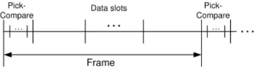
Pick-Compare Data slots

Frame

Pick-Compare

(a) Frame-based implementation: data transmis-sion begins after power allocation is updated, and uses the same power allocation over multi-ple slots. Data channel Data slots Low bandwidth control channel Pick-Compare slots

(b) Control-channel based implementation: sep-arate low bandwidth control channel is used for power allocation, in parallel with data channel. Fig. 1. Frame-based and control-channel based implementations

Using (10) and (15), the conditional expectation of T -step Lyapunov drift in (7)-(8) can be bounded as ∆T(t)≤ −2T × { 1− ρ − γ1− (1 − γ1)γ2− 1 δ1T − δ 2T } W∗(t) + B4

where B4 = B1 + 2B3 + 2B2 is a finite number.

Now, the proof can be completed by choosing T = √

1/(δ1δ2), and applying the inequality (14) and the

condition ρ < 1− γ1− (1 − γ1)γ2− 2

√ δ2

δ1.

When γ1is 0, i.e., when a new power vector is optimal

with probability δ1, the obtained throughput mainly

depends on the comparison performance (γ2).

How-ever, the throughput loss increases as γ1increases. In

case of perfect comparison (i.e., γ2 = 0 and δ2 = 0),

the throughput loss depends only on the optimality loss in the random power allocation. In brief, our randomized power control framework can achieve nearly 100% throughput if we can develop a power allocation policy (RAND-POW) and a comparison al-gorithm (DECIDE) satisfying conditions C1 and C2 with small γ1, γ2 and δ2. In the rest of the paper, we

focus on developing such algorithms. In particular, in Section 4 we develop a random power allocation policy that satisfies C1 and in Section 5 we develop a comparison algorithm that satisfies C2.

3.3 Frame-based Implementation

In this section, we discuss some issues arising in the implementation of our randomization framework. First, the RAND-POWstep can be easily implemented as it is easy to generate a random power vector in a distributed manner, as we demonstrate in Section 4. For the DECIDE phase, each node has to estimate

the global weights qT_{r in order to make the same} decision on the selection of the current power allo-cation. In small networks, a centralized entity may exist (e.g., base station in cellular networks), hence

comparison and decision can be implemented in a centralized manner. In large networks, however, such a centralized comparison is prohibitive and we adopt gossiping for distributed comparison.

In the proof of Theorem 1, we assumed for sim-plicity that the power allocation is updated for each data transmission slot by running the RAND-POWand

DECIDE steps. However, it may not be practical to

run these two steps on a slot-by-slot basis because the DECIDE step may require a significant amount of communications. In fact, this assumption can be easily relaxed by running the RAND-POW and DECIDE on a frame basis as shown in Fig. 1(a); where they are performed for every multiple data transmission slots so that the same power allocation is kept for multiple data slots. By doing so, the control overhead can be significantly reduced. Moreover, it was shown in [4] that this frame-based scheduling still achieves throughput optimality as long as the RAND-POW

and DECIDEsteps are performed at regular intervals.

Alternatively, the power control algorithm can be done on a separate low bandwidth control channel, in parallel with data transmission, as shown in Fig. 1(b). Again, throughput optimality can be achieved as long as a new power allocation is generated at regular (finite duration) intervals. The advantage of this implementation over the frame-based is clear, that is, the data transmission does not need to wait until the update of power allocation is finished, and consequently it will achieve better performance.

4

R

P

A

We present a power allocation policy RAND-POW

that satisfies C1, i.e., finds with positive probability a power vector within a small factor of the optimal value in (5). The problem (5) is to maximize

p∗= arg max p∈F ∑ a∈V ∑ b_{∈V (a)} qab× log  1 + gabpab nb+gab ∑ i∈V (a)\b pai+ ∑ i̸=a gib ∑ j∈V (i) pij   , (16) where F = {p ≥ 0 : ∑b∈V (a)pab ≤ Pamax,∀a ∈ V }. Clearly, the new power vector ˜p in RAND-POW is desired to be as close to p∗ as possible, and hence, identifying the optimality properties of (16) would be helpful for generating such ˜p. The following lemma characterizes some useful properties of p∗.

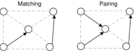
Lemma 2: Under the optimal power allocation p∗, (i) A node does not transmit while receiving, and

vice versa,

(ii) A node transmits to at most one of its neighbors.

Proof: Recall the assumption gaa =∞, ∀a. Under this assumption, if a node transmits while trying to receive, it will achieve zero rate due to infinite interference. Hence, at optimal p∗, case (i) does not happen.

Matching Pairing

Fig. 2. Matching: either (single) transmission or reception is allowed for each node. Pairing: node can receive from multiple neighbors but transmitting to multiple neighbors are not allowed.

To prove (ii), let p∗a = ∑

b∈V (a)p∗ab, i.e., p∗a is the total power transmitted by node a at the optimal allocation. It is obvious that solving the problem (16) with the additional constraints∑b∈V (a)pab= p∗a,∀a will result in the same optimal solution. Hence, the objective function in (16) can be written as

∑ a ∑ b_{∈V (a)} qablog   1 + gabpab nb+ gab(p∗a− pab) + ∑ i_̸=a gibp∗i    . Clearly, changing transmit power pab,∀b ∈ V (a) un-der fixed total power does not affect the mutual interference, but only changes the self-interference. Hence, the new optimization problem can be solved separately with respect to each node, i.e., for each a, we only need to maximize

∑ b∈V (a) qablog   1 + _n gabpab b+ gab(p∗a− pab) + ∑ i̸=a gibp∗i    subject to p ≥ 0 and ∑b∈V (a)pab = p∗a. Since this function is strictly convex in [pab,∀b ∈ V (a)], it is maximized at a corner point, i.e., pab = p∗a for some

b ∈ V (a) and zero for all others. This shows that it

is optimal for each node to transmit to at most one neighbor.

According to Lemma 2, at an optimal allocation, a node is not allowed to transmit to multiple neighbors, and to be a transmitter and receiver simultaneously. Note, however, that it is possible for a node to re-ceive from multiple transmitters. This is in contrast to a matching in which a node cannot be shared by multiple edges. For ease of exposition, we define the notion of a pairing as follows:

Definition 2: Assume that the tail and the head of

a directed edge denote a transmitter and a receiver respectively. A directed subgraph of G is called a

pairing if it satisfies (i) and (ii) in Lemma 2.

Note that a pairing is different from a matching because it allows a node to be shared by multiple edges. Figure 2 shows an example of matching and pairing

4.1 Transmitter-Receiver Pairing

From Lemma 2, it is clear that finding a power allo-cation can be decomposed into two steps. First, find a pairing, and then select the transmit power levels

Algorithm 2 RAND-PAIR

1: Each node a decides to be a transmitter w.p. 1/2 and a receiver w.p. 1/2, and initializes Iab = 0,∀b ∈ V (a).

2: Each transmitting node a sends a pair-request

mes-sage (PQM) to one of its neighbors in V (a) uni-formly at random.

3: If node b receives a PQM, one of the following happens:

(i) If node b is a receiver, then it accepts the re-quest and sends a pair-rere-quest-accepted mes-sage (PAM) to node a.

(ii) Otherwise, ignore the PQM and nothing hap-pens for node a.

4: If node a receives a PAM from node b, set Iab= 1, meaning that node b is a receiver of node a.

for the given pairing. Since there is a finite number of pairings, and at least one of them is optimal, it is easy to generate an optimal pairing with positive probability. One such algorithm is given by RAND -PAIR(see Algorithm 2). Let Iab= 1if node a transmits to its neighbor b, and 0 otherwise. The goal of RAND

-PAIRis to generate a vector I = [Iab, b∈ V (a), a ∈ V ] satisfying the pairing constraints. To do this, each node a decides to be a transmitter with probability (w.p.) 1

2 and a receiver w.p. 1

2. Then, each transmitting

node a sends a pair-request message to one of its neighbors b. If b decided to be a receiver, it accepts the request and sends an acceptance message. Otherwise, it is ignored and nothing happens. Once node a receives the acceptance message, it updates Iab to

Iab = 1. This algorithm has O(1) computation and communication complexity, and will find an optimal pairing with positive probability, as stated in the following lemma.

Lemma 3: Algorithm RAND-PAIR finds an optimal pairing with probability at least (4N )−N.

Proof: See [31].

Note that in the interference graph model, a new scheduling should be a max-weight matching (or independent set in general) with positive probability. Because the max-weight matching is one of maximal matchings, and such a probability can be increased by performing multiple iterations until the obtained matching becomes maximal. However, in our case, maximal pairing1 _{may not be always optimal. Hence,}

performing multiple iterations does not necessarily enhance the probability of being optimal, and further it may not guarantee that the obtained pairing has a positive probability of being optimal.

1. A pairing I is maximal if adding a link (not in I) to I makes it no longer a pairing

Algorithm 3 RAND-PSEL (for given pairing I)

1: Each node a initializes ˜pab= 0,∀b ∈ V (a).

2: Every paired transmitting node a does the following: (i) Select a number, say u, from [0, Pmax

a ] uni-formly at random, and set ˜pab= ufor b such that Iab= 1.

4.2 Power Level Selection

Now what remains is to select a power level which together with RAND-PAIR satisfies C1. Recall that RAND-PAIRgenerates a pairing I = [Iab, b∈ V (a), a ∈

V ]. Given this pairing, the problem (16) is rewritten by: p∗(I) = arg max p∈F ∑ a∈V ∑ b:Iab=1 qablog   1 + gabpab nb+ ∑ ı̸=a ∑ j:Iij =1 gibpij   . (17) Notice that the self-interference has been removed and the mutual interference has been simplified due to the constraints (i) and (ii) in Lemma 2. Since the pairing

I found by RAND-PAIR has a positive probability of being optimal, the condition C1 can be satisfied if a power level is selected such that it is within a factor of the objective in (17) with positive probability. To meet this requirement, Algorithm RAND-PSELsimply chooses power levels uniformly at random. In par-ticular, each transmitting node a randomly selects its transmit power from the feasible region, i.e., [0, Pmax

a ]. This random power selection meets the requirement as shown in the following lemma. Assume Pmax

a =

1,∀a.

Lemma 4: For any ϵ∈ (0, 1), Algorithm RAND-PSEL

generates a power vector ˜p such that ˜p∈ B(p∗(I), ϵ) with probability at least

( ϵ √ N )N , where B(p∗(I), ϵ) = {p ∈ F : ||p − p∗_(I)|| 2≤ ϵ}. Proof: See [31].

Note that this lemma can be easily extended to the case of general Pmax

a . Combining Lemmas 3 and 4, we can show that Condition C1 can be satisfied by RAND-PAIRand RAND-PSEL.

Theorem 2: Choosing a power allocation according

to RAND-PAIRand RAND-PSELsatisfies C1 with arbi-trarily small γ1> 0and positive δ1which is a function

of γ1.

Proof: Let f (p) be the objective function in (17),

and consider an arbitrary γ1 ∈ (0, 1). Due to the

continuity of f (p), there exists ϵ > 0 such that

f (p) ≥ (1 − γ1)f (p∗(I)) for any feasible p such that

||p − p∗_{(I)|| ≤ ϵ. Let I be a pairing generated by} RAND-PAIRand ˜pbe a power vector obtained through RAND-PSEL, given pairing I. Let I∗ be an optimal

pairing. Then, it follows that Pr[qT_{r(˜p)≥ (1 − γ}

1)qTr(p∗)

]

= Pr [f (˜p)≥ (1 − γ1)f (p∗(I))|I = I∗] Pr[I = I∗]

≥ Pr [||˜p − p∗_{(I)||2≤ ϵ|I = I}∗_{] Pr[I = I}∗_]

≥(_√ϵ N )N · (4N)−N _{= (} ϵ 4N3/2) N_,

where the last inequality is due to Lemmas 3 and 4. Therefore, the power allocation obtained by RAND -PAIRand RAND-PSELachieves at least (1−γ1)fraction

of optimal value of problem (16) with probability at least δ1= (_4Nϵ3/2)

N _{> 0, satisfying Condition C1.} Therefore, the optimality loss γ1 can be arbitrarily

small (with small enough ϵ and thus small probability

δ1). According to Theorem 1, the throughput loss due

to this optimality loss (γ1) under our power allocation

is negligible, as long as δ2≪ δ1.

Remark: Theorem 2 implies that the random power allocation hits a near optimal solution in every (4N_ϵ3/2)N _{slots (in average sense). As a consequence} it can experience large delay or network backlog, although our work in this paper focuses on the long-term throughput performance. In fact, recent results in [33] show that there may not exist a polynomial time (deterministic or randomized) throughput opti-mal policy for NP-hard scheduling problem such that it achieves polynomial network backlog. The power allocation problem (5) contains a maximum weight independent set problem [24]. Hence, any polynomial time power allocation policy that takes on the prob-lem (5) will experience large delay, as our random power allocation algorithm will. This implies that our random power allocation algorithm may not scale very well as the network size grows. As mentioned above, in this paper, we focus on the throughput performance, and we leave this delay and scalability issue as future research.

5

C

A

The goal of the DECIDE step is to choose a power allocation p(t) by selecting one of the two power allocations p(t− 1) and ˜p(t), so that Condition C2 can be satisfied. Such a selection is easy in a cen-tralized setting; namely, a central entity can com-pare q(t)T_{r(p(t− 1)) and q(t)}T_{r(˜p(t)), pick the one} having larger value, and disseminate the selection to every node. In small networks, such a centralized comparison might be possible, or a spanning tree could be computed in a distributed manner and used for the comparison [5]. However, in large networks, such a centralized computation is prohibitive. For this reason, we develop a distributed DECIDE policy by using randomized gossiping [32]. It consists of two procedures, COMPARE and AGREE. The COMPARE

procedure estimates the objective values achieved under the new and old power allocations, and the AGREE procedure uses these estimates to make a

unanimous decision on the selection of current power allocation.

Let xnew

b (0) and xoldb (0)be the weighted (receiving) rates at node b under the new power ˜p(t) and old power p(t− 1), respectively. Then, they can be ex-pressed as xnew b (0) = ∑ a_∈V qab(t)rab(˜p(t)) and xoldb (0) = ∑ a∈V qab(t)rab(p(t− 1)). Let Xnew = ∑ a∈V xnewa (0) and X_old= ∑ a∈V xold

a (0), i.e., Xnewand Xoldare the objective

function values under the newly generated power vector and the old power vector, respectively. The

DECIDE step must choose the new power allocation

if Xnew > Xold, and the old one if Xnew ≤ Xold.

This can also be accomplished using the average values ¯X_newand ¯X_oldinstead of Xnewand Xold, where

¯

X_new = X_new/N and ¯X_old = X_old/N. Therefore, if every node can compute an accurate estimate of ¯X_new

and ¯X_old, they will be able to make a decision leading to C2. A randomized gossiping algorithm is used to estimate ¯X_new and ¯X_old. Note that gossiping has been used extensively for computing averages (See [32], [34] and references therein).

Typically, gossiping generates a matching for each iteration. Let xa(k) be the value at node a after iteration k. The initial value is thus xa(0) and the global average is∑axa(0)/N. If any two nodes a and

b share the same link under the current matching, then they update their values to their average, i.e.,

xa(k + 1) = xb(k + 1) = xa(k)+x₂ b(k). Gossiping keeps generating a random matching for this averaging operation, and every node eventually obtains an esti-mate of the global average∑axa(0)/N. In this paper, we use a random matching policy in [32] that works as follows. Let d(a) be the degree of node a, i.e.,

d(a) =|V (a)| and d∗ be the maximum node degree, i.e., d∗= maxa∈V d(a). Each node a decides to be ac-tive with probability (w.p.) 1

2 and inactive w.p. 1 2. An

active node a does nothing w.p. 1−d(a)_d∗ , and randomly

contacts one of its neighbors w.p. d(a)_d∗ 2. Consider an

inactive node b. If b is contacted by node a while it has not been contacted by any other, then nodes a and b average their values w.p.(1−_2d1∗

)d∗−d(b)

. Otherwise, nothing happens for a.

5.1 COMPAREand AGREE

The COMPAREprocedure estimates the averages ¯X_new

and ¯X_old using the gossiping described above, and is shown in Algorithm COMPARE. Note that at each iteration, a matching is generated and any two nodes sharing a link in that matching average their values. Note also that the same matching is used for new and

2. Under the algorithm COMPARE, each active node a has 1₂d(a)

inactive neighbors in average. Hence for better chance of matching, it is desirable for an active node with high degree to make an attempt to match with high probability, while a node with low degree is desired to attempt with low probability. This is why the contact probability is proportional to the node degree.

Algorithm 4 COMPARE

1: For iteration k = 1, ..., K, do the following: (i) Each node a updates xnew

a (k) = xnewa (k− 1) and xold

a (k) = xolda (k− 1).

(ii) Each node decides to be active w.p. 1/2 and inactive w.p. 1/2. An active node a does nothing w.p. 1 − d(a)_d∗ , and contacts one of

its neighbors uniformly at random (i.e., with equal probability 1

d∗).

(iii) If node b is contacted, one of the following happens:

(b) If b is inactive and has not been con-tacted, they average as xnew

a (k) = xnewb (k) = xnew_a (k−1)+xnew_b (k−1)

2 and xolda (k) = xoldb (k) = xold_a (k−1)+xold_b (k−1) 2 w.p. ( 1− 1 2d∗ )d∗−d(b) . (c) Otherwise, b ignores the contact and

noth-ing happens for a.

Algorithm 5 AGREE

1: Run gossiping for ˜K iterations to estimate the average ∑

a∈V

za(0)/N.

2: Each node a selects the new power if za( ˜K)≥ 1, and the old one otherwise.

old values. After K iterations, every node will obtain the estimates of new and old average values xnew

a (K) and xold

a (K).

If the estimates are exact, a unanimous decision satisfying C2 can be easily made since every node a will have xnew

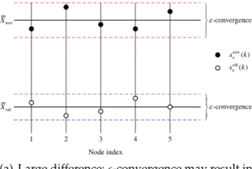
a (K) > xolda (K) (or xnewa (K)≤ xolda (K)). Such a unanimous decision can also be guaranteed if the estimates are highly accurate, provided that the difference| ¯X_new− ¯X_old| is sufficiently large. However,

in the case of small difference, decisions can be mixed even under highly accurate estimation (See Fig. 3), which can lead to the violation of C2. An additional procedure is thus needed to ensure that every node makes the same and right decision.

The AGREE procedure keeps the decision made

by COMPARE if it is unanimous. Otherwise, it keeps

the old power allocation. Note that in the case of small difference, this selection policy will not incur big losses in throughput because there is only a small difference between selecting either the new or the old power allocation. To do this, the AGREE procedure uses the estimates xnewa (K) and xolda (K) as follows. Each node a initiates a variable za(0) as follows:

za(0) = { 1 if xnew a (K) > xolda (K) 0 if xnew a (K)≤ xolda (K).

Namely, za(0)is equal to 1 if node a prefers the new power allocation and 0 otherwise. It runs gossiping for ˜K iterations (as in COMPARE) to estimate the

average ¯Z = ∑

a_∈V

new ( ) a x k new X H-convergence ½ ° ¾ ° ¿ old X ½°¾H-convergence °¿ Node index 1 2 3 4 5 old_{( )} a x k

(a) Large difference: ϵ-convergence may result in unanimous decision new ( ) a x k new X H-convergence ½ ° ¾ ° ¿ old X ½°¾H-convergence °¿ Node index 1 2 3 4 5 old_{( )} a x k

(b) Small difference: decisions can be mixed even under ϵ-convergence

Fig. 3. Impact of difference| ¯Xnew− ¯Xold| on unanimous decisions

decides to use the new power if za( ˜K) = 1 and the old one otherwise, where za(k)is the value at node a after iteration k. Note that if za(0)’s are all zero or all one, then the convergence and unanimous decision is guaranteed immediately. We will show that this is the right decision. If there is a mixture of decisions at the end of COMPARE, the AGREEprocedure tries to keep the old power allocation. The following lemmas show a unanimous decision is the right decision; hence justifying the AGREE.

Lemma 5: Suppose that there was an agreement

after COMPARE, i.e., za(0)’s are all zero or all one. Then, it is the right decision regardless of the values of ¯X_new and ¯X_old in that the power allocation se-lected based on za(0)’s achieves the objective value of max{X_new, X_old}. As a consequence, unanimous wrong

decisions cannot happen after COMPARE.

Proof: To prove Lemma 5, we need the following

lemma. Again, let xa be xnewa , xolda or za.

Lemma 6: For every k≥ 0, the sum is conserved as

∑ a∈V xa(k) = ∑ a∈V xa(0).

Proof: Let xa(k)and x(k) be the value of node a after iteration k and its vector, respectively. Denote by

M (k) the matching found in iteration k. The update of node values can be expressed as a linear equation by

x(k + 1) = W (k)x(k), (18) where W (k) is an N× N matrix given by

W (k) = I− ∑

(a,b)∈M(k)

(ea− eb)(ea− eb)T

2 , (19)

where I is the identity matrix and ei is the i-th element vector whose i-th coordinate is 1 and all

others are zero. The first term in W (k) corresponds to the original value of each node and the second term describes the change from the original value. For example, when node a averages with b, its new value becomes 12xa(k) + 1 2xb(k) = xa(k)− 1 2xa(k) + 1 2xb(k),

where the first term corresponds to I and the last two terms correspond to the second term in (19). Note that the matrix W (k) is doubly stochastic, and as a consequence, the following holds:

∑ a∈V xa(k + 1) = ⃗1T · x(k + 1) = ⃗1T_{W (k)x(k)} = ⃗1T _{· x(k) =} ∑ a∈V xa(k). The third equality is due to the fact that W (k) is doubly stochastic. This proves the lemma.

We now prove Lemma 5. Under the assumption of unanimous decisions after COMPARE, there can be only two cases including (i) xnew

a (K) > xolda (K),∀a or (ii) xnewa (K) ≤ xolda (K),∀a. Suppose case (i), in which case every node selects the new power. Then, it follows that ∑ axnewa (K) > ∑ axolda (K) ⇒∑axnewa (0) > ∑ axolda (0),

where the second line is due to Lemma 6. Therefore, selecting the new power is the right decision. Case (ii) can be proved similarly.

Therefore, it is desirable to keep any unanimous deci-sion made after COMPARE, because the better power allocation is always selected under such a decision. This justifies the AGREEprocedure that always keeps unanimous decisions made after COMPARE.

We now analyze and prove that the combination of

COMPARE and AGREE can satisfy Condition C2. For

the proof, we need to define some parameters. Let

x(k) be the vector of xa(k)’s and ¯X = ∑

axa(0)/N, where xa can be xnewa , xolda or za.

Definition 3 (ϵ-convergence time, [32]): For given δ >

0, the ϵ-convergence time K(ϵ, δ) is defined by

K(ϵ, δ) = sup x(0) inf { k : Pr [ ||x(k) − ¯X⃗1|| ||x(0)|| ≤ ϵ ] ≥ 1 − δ } (20) where|| · || is l2-norm.

Briefly, the ϵ-convergence time is the time until the estimation vector x(k) falls into the ϵ-neighborhood (in relative sense) of the average vector ¯X⃗1with high probability.

Assumption 1: Fix arbitrary γ2, δ2∈ (0, 1). Consider

positive constants ˆϵ, ϵ, δ, ˜ϵ, ¯ϵand assume the following: 0 < ˆϵ≤ γ2 2−γ2, ϵ = ˆ ϵ N, 0 < δ≤ δ2 2 0 < ˜ϵ <_N1₋₁, ¯ϵ = _Nϵ˜.

Assume further that K = K(ϵ, δ) in COMPARE and

˜

K = K(¯ϵ, δ)in AGREE.

Let ¯X_agr be the average objective value achieved by the above described DECIDE algorithm that runs

COMPAREand then AGREE. It can be proved that this policy satisfies C2 as shown in Theorem 3.

Theorem 3: Consider any γ2, δ2 ∈ (0, 1). Under

As-sumption 1, the DECIDE algorithm (COMPARE and AGREE) achieves

Pr[ ¯X_agr≥ (1 − γ2) max{ ¯Xnew, ¯Xold}] ≥ 1 − δ2.

Proof: See Section 5.2.

Remark: As seen above, the ϵ-convergence time

K(ϵ, δ) is a critical parameter because Condition C2 can be guaranteed after ϵ-convergence time in COM

-PARE and AGREE. It is known that in a line or ring topology, it is given by Θ(−N2_{log(ϵδ)) [35].}

More-over, in a complete graph, it is given by K(ϵ, δ) = Θ(− log(ϵδ)) [32]. In wireless networks, the topol-ogy can be controlled by adjusting the coding and transmission rate. That is, if a strong coding is used with low transmission rate, then the communication range can be increased (for the purpose of control signalling only). This will make the topology closer to a complete graph. In particular, a small network could be made a complete graph. Hence, if this is used for gossiping, the ϵ-convergence time will be substantially improved3_{. The convergence time can}

be further improved by exploiting the geographic in-formation. In [37], [38], geographic gossip algorithms were developed such that their convergence time is

O(N ). Clearly, this is order optimal for network-wide averaging, and therefore, the gossiping-based comparison can be a practical solution in real wireless networks.

Remark: We briefly discuss the total overhead of our algorithm. Recall that our algorithm consists of RAND-POW and DECIDE. In RAND-POW, O(N ) and

O(1)computations are needed respectively for RAND -PAIR, and RAND-PSEL. The DECIDE step runs two rounds of gossip algorithm which requires O(N3₎

computations in the worst case [32]. Therefore, our algorithm requires O(N3_{)computations in total.}

5.2 Proof of Theorem 3

The theorem is proved in three steps. First, in Sec-tion 5.2.1, we analyze the case of large difference

| ¯Xnew− ¯Xold|. In particular, we show that a unanimous

decision can be easily made, given that every has obtained a good estimate (ϵ-convergence) of averages. Since any unanimous decision made after COMPARE

is the right decision, the probability of right decision is the probability of ϵ-convergence in COMPARE. We show that this probability is high. Second, in Section 5.2.2, we deal with the case of small difference, where even a good estimate can possibly result in mixed decisions. The key to dealing with this case is that

3. In fact, the techniques used in [35], [36] for analyzing conver-gence time show that as the number of disjoint paths increases, the convergence speed increases. Hence, such a topology control will enhance the convergence speed. More details can be found in [31].

selecting either the new or old power allocation is not a bad choice due to| ¯Xnew_{≈ ¯X}old_{|. We show that}

the AGREE procedure attains a unanimous decision with probability, which in this case implies a fairly good choice. Finally, Section 5.2.3 combines these two results to show that COMPARE and AGREE will

select the power allocation that achieves almost the maximum of new and old objective values with high probability.

5.2.1 The Case of Large Difference

Let us first delineate between large and small dif-ferences. Consider an arbitrary ˆϵ ∈ (0, 1), and let ϵ = ˆϵ/N. Recall the definition of K(ϵ, δ) in (20). It can be easily shown that under Algorithm COMPARE, for any k≥ K(ϵ, δ),

|xnew

a (k)− ¯Xnew| ≤ ˆϵ ¯Xnew,∀a ∈ V

|xold

a (k)− ¯Xold| ≤ ˆϵ ¯Xold,∀a ∈ V (21)

with probability at least 1− δ. Define E1 as the event

that (21) is satisfied, under the assumption that K =

K(ϵ, δ) in Algorithm COMPARE. Then, it is obvious

that Pr[E1]≥ 1−δ. Define E2as the event4that ¯Xnew> 1+ˆϵ

1−ˆϵX¯old or ¯Xnew≤ 1−ˆϵ

1+ˆϵX¯old. Then, its complementE C

2

is the event that 1_1+ˆ−ˆϵ_ϵX¯_old < ¯X_new ≤ 1+ˆ_1−ˆϵϵX¯_old. Note that the eventE2basically indicates that the difference

between the old and new average values is relatively large, whereasEC

2 indicates that they are fairly close.

These two eventsE2 andE2C respectively define large

and small differences. In the following, we will see how these two events affect the performance of our decision policy.

Consider a naive policy Π such that each node a decides its power based on its own estimates obtained by running COMPARE, that is, it switches to the new

power if xnew

a (K) > xolda (K) and keeps the old one otherwise.

Lemma 7: Assume K = K(ϵ, δ) in Algorithm COM -PARE. Then, the policy Π

Pr[ ¯XΠ≥ max{ ¯Xnew, ¯Xold}|E1,E2] = 1,

where ¯XΠis the average objective value of the power

vector selected under the policy Π.

Proof: Given E1, (21) holds, and consequently it

follows that for all a, (1− ˆϵ) ¯X_new− (1 + ˆϵ) ¯X_old

≤ xnew

a (K)− xolda (K)≤ (1 + ˆϵ) ¯Xnew− (1 − ˆϵ) ¯Xold.

Further, givenE2, we have ¯Xnew> 11+ˆ−ˆϵϵX¯oldor ¯Xnew≤ 1_−ˆϵ

1+ˆϵX¯old. In the first case, the above sandwich in-equality implies xnew

a (K) > xolda (K),∀a. Consequently, every node will select the new power under the policy Π so that ¯XΠ = X¯new. Note that this is the right

decision because ¯X_new> ¯X_oldin this case. The second case can be proved similarly.

The following is a consequence of Lemma 7. Corollary 1: Given EC 2, i.e., if 1_−ˆϵ 1+ˆϵX¯old < X¯new ≤ 1+ˆϵ

1−ˆϵX¯old, the policy Π can result in mixed decisions

even after ϵ-convergence.

Lemma 7 shows that when the difference between ¯

X_new and ¯X_old is sufficiently large, the desired selec-tion can be made easily based solely on the COMPARE

procedure. On the other hand, according to the above corollary, if they are too close, the decisions can be mixed, that can possibly lead to the violation of C2. Note also that as the accuracy of estimation increases (i.e., ˆϵ decreases), the region of mixed decisions di-minishes.

5.2.2 The Case of Small Difference

So far we have seen that when the difference is large (i.e., given E2), a unanimous decision can be easily

made right after COMPARE. Moreover, any unanimous decision is kept by AGREE, and hence, Lemma 7 also hold for AGREE. This subsection studies the case where the decisions are mixed after COMPARE, in particular when the difference is small.

Recall that if za(0)’s are all zero or all one, then the convergence and the right decision are guaranteed immediately under the decision algorithm AGREE

(See Lemma 5). Hence, assume that such a case has not happened, so that there is a mixture of nodes with za(0) = 0 and za(0) = 1. Consider any ˜ϵ ∈ (0, 1/(N−1)) and let ¯ϵ = ˜ϵ/N. Then, as argued in (21), after ˜K = K(¯ϵ, δ)iterations in AGREE, every node a

will obtain

(1− ˜ϵ) ¯Z ≤ za( ˜K)≤ (1 + ˜ϵ) ¯Z (22) with probability at least 1−δ. Consequently, the above inequality implies 0 < za( ˜K) < 1,∀a since 1/N ≤ ¯Z≤ (N − 1)/N and ˜ϵ < 1/(N − 1). Hence, every node will acknowledge that there are mixed decisions, and hence they will decide to use the old power.

Let E3 denote this event, i.e., E3 is the event that

every node obtains ˜ϵ approximation of ¯Z (as in (22)) under the assumption that ˜K = K(¯ϵ, δ). Note that Pr[E3] ≥ 1 − δ. The following lemma shows the

performance of AGREEunder some conditions.

Lemma 8: Let ¯X_agr be the average objective value achieved by AGREE. Then,

Pr[ ¯X_agr≥ (1 − 2˜ϵ/(1 + ˜ϵ)) max{ ¯X_new, ¯X_old}|E₂C,E3] = 1.

Proof: Note first that givenE3, the AGREE policy

will result in agreed decisions. If za(0)’s were all zero or one, then it follows from Lemma 5 that ¯X_agr = max{ ¯X_new, ¯X_old}. If this was not the case, then every

node will select the old power givenE3; so that ¯Xagr=

¯

X_old. Further, given EC

2, we have 11+ˆ−ˆϵϵX¯old < ¯Xnew ≤

1+ˆϵ

1−ˆϵX¯old. Consequently, it follows that ¯Xagr = ¯Xold ≥ 1_−˜ϵ

1+˜ϵmax{ ¯Xnew, ¯Xold}. Therefore, the agreed decisions are made achieving at least 1− 2˜ϵ

1+˜ϵ of the maximum of old and new values.

Lemma 8 implies that when the case of small differ-ence can be addressed by the AGREEprocedure. That is, if the decisions were unanimous after COMPARE, they are right decisions and kept by AGREE. Even if the decisions are mixed, the AGREE procedure can guarantee almost the maximum of new and old objective values with high probability.

5.2.3 Combining All The Results

We now combine all the above results to complete the proof. For any trivial event A (i.e., event having zero probability measure), assume the convention P (·|A) = 0 where P (·) is probability measure. We will use the following relationship for any events A, B, C:

P (A|B) = P (A|B, C)P (C|B) + P (A|B, CC)P (CC|B). (23) Recall E1, E2, E3 are respectively the events of

ϵ-convergence in COMPARE, relatively large difference between ¯X_newand ¯X_old, and ¯ϵ-convergence in AGREE.

Let ¯X_max= max{ ¯X_new, ¯X_old}. First, note that

Pr[ ¯X_agr≥ (1 − γ2) ¯Xmax]

= Pr[ ¯X_agr≥ (1 − γ2) ¯Xmax|E1]· Pr[E1]

+ Pr[ ¯X_agr≥ (1 − γ2) ¯Xmax|E1C]· Pr[E1C]

≥ (1 − δ) Pr[ ¯X_agr≥ (1 − γ2) ¯Xmax|E1],

where the inequality follows from the facts that the second term is nonnegative and Pr[E1]≥ 1 − δ. Using

the relationship (23), the last line can be rewritten as = (1− δ){Pr[ ¯X_agr ≥ (1 − γ2) ¯Xmax|E1,E2]· Pr[E2|E1]

+ Pr[ ¯X_agr≥ (1 − γ2) ¯Xmax|E1,E2C]· Pr[E2C|E1]

}

≥ (1 − δ) {Pr[E2|E1]

+ Pr[ ¯X_agr≥ (1 − γ2) ¯Xmax|E1,E2C]· Pr[E2C|E1]

}

≥ (1 − δ) Pr[ ¯X_agr≥ (1 − γ2) ¯Xmax|E1,E2C],

The second inequality follows from Lemma 7, and the last inequality follows from the fact Pr[E2|E1] +

Pr[EC

2|E1] = 1. Similarly to the above (where (23) was

applied and the second term was removed for pro-ceeding the inequality), the last line can be rewritten as

≥ (1 − δ) Pr[ ¯X_agr ≥ (1 − γ2) ¯Xmax|E1,E2C,E3]· Pr[E3|E1,E2C].

Recall Pr[E3]≥ 1 − δ, and this is true regardless of the

initial value z(0). The events E1 and E2C only affect

the initial value, hence the conditional probability Pr[E3|E1,E2C]is also no less than 1−δ. By Assumption

1, we also have (1− γ2) ≤ (1 − _1+˜2˜ϵ_ϵ). The above

inequality is then rewritten as

≥ (1 − δ)2_{Pr[ ¯X}

agr≥ (1 −1+˜2˜ϵϵ) ¯Xmax|E1,E C

2,E3].

The proof is completed by noting that Lemma 8 holds even if it is additionally conditioned onE1and using

δ≤ δ2

5.3 Sign-wise Convergence

In order for a unanimous decision to be made after running COMPARE, every node a has to obtain the

estimate such that xnew

a (k) > xolda (k) (or xnewa (k) ≤

xold_a (k)). Without loss of generality, we assume ¯X_new>

¯

X_old. Obviously, the ϵ-convergence is not a necessary condition for xnew

a (k) > xolda (k),∀a. Therefore, the ϵ-convergence time is a conservative lower bound in that a unanimous decision can be possibly made without having ϵ-approximation of the actual average. This has led us to define a new concept of sign-wise

con-vergence (or s-concon-vergence).

Definition 4: A real-number vector x is said to be uniform in sign (u.i.s.) if x > 0 (or x≤ 0) component

wise.

Definition 5 (s-convergence time): For a sequence of

vectors{x(k)}, the sign-wise convergence time Ks_(δ)is defined by

Ks(δ) = inf{k ≥ 0 : Pr [x(k) is u.i.s. ] ≥ 1 − δ} . (24) Let xdif

a (k) = xnewa (k)− xolda (k), then a unanimous decision can be made when the vector xdif_{(k)is u.i.s.}

The following result is obvious.

Lemma 9: Note that once a sequence{xdif_(k)}

gen-erated by Algorithm COMPARE becomes u.i.s., it will remain u.i.s. forever.

Proof: Suppose that xdif_{(k) is u.i.s, and consider}

any two nodes a,b. Since the vector is u.i.s., we have

xnew_a (k) > xold_a (k) and xnew

b (k) > xoldb (k). If they average in the next iteration, then

xnew_a (k + 1) = xnewa (k)+xnewb (k)

2 >

xold_a(k)+xold_b (k)

2 = xolda (k + 1), and the same is true for node b. This completes the proof.

As a consequence, after any K≥ Ks_(δ

2)iterations in

COMPARE, a decision can be made such that C2 is

satisfied with γ2= 0. Now, it remains to identify the

value of Ks_{(δ) in terms of network parameters. Let} ¯

X_dif= ¯X_new− ¯X_old, then by assumption ¯X_dif> 0.

Lemma 10: The following is a sufficient condition

for the sign-wise convergence of vector xdif_(k):

||xdif_{(k)− ¯X} dif⃗1|| < √ N ¯X_dif ( N α2 − 1 )1/2 , (25) where α is a constant in (1,√N ).

Proof: For notational convenience, drop all the

indices and consider an N -dimensional vector x such that∑ixi = N ¯X. We want to find the condition when

x > 0component wise. To get some intuition, we start from the case of N = 2. In this case, the condition is easily obtained as x1x2 > 0 (Since we are assuming

¯

X_new > ¯X_old, the case of x1 ≤ 0 & x2 ≤ 0 cannot

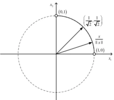
happen), but this form of condition is not easy to extend to higher dimension. Consider the normalized vector x

||x||, which has exactly the same properties as

xin terms of sign-wise convergence. This vector lies on the unit circle as shown in Fig. 4. Observe that any

1 x 1 1 , 2 2 § · ¨ ¸ © ¹  1, 0 2 x  0,1 || || x x

Fig. 4. Sign-wise convergence condition in 2-dimension

u.i.s. vector lies on the solid line, and the vector_√1 2⃗1 at

its center. We call this standard vector. It is easy to see that if the inner product of standard vector and x

||x|| is greater than certain value, then x is u.i.s. That value can be easily computed as _√1

2, hence the condition is

written as 1 √ 2⃗1· x ||x|| > 1 √ 2. (26)

Expanding and rearranging the above condition yields x1x2 > 0. In this case, this is a necessary and

sufficient condition (given that x1≤ 0 & x2≤ 0 cannot

happen).

For higher dimension, we take similar approach. First, the standard vector _√1

N⃗1 will lie at the center of the space where all the u.i.s. vectors exist. Similarly to the 2-dimensional case, it is obvious that any u.i.s. vector can be described as

1 √ N⃗1· x ||x|| > α √ N ⇒ α||x|| < ∑ i xi. (27) Notice that this a natural generalization of (26), except for α. For N = 2, α was 1. However, we can show that

αshould be greater than 1 as below.

Lemma 11 ( [31]): Assume N ≥ 3. In order for the

condition (27) to describe u.i.s vectors, it should be 1 < α <√N.

Squaring both side of the inequality (27) and using the condition∑ixi= N ¯X yields

||x||2 _< N2_X¯2 α2 ||x − ¯X⃗1|| < √N ¯X(N α2 − 1 )1/2 .

This proves the lemma since the vector xdif(k)satisfies all the conditions assumed on x here.

Since the same matching is used for averaging new and old values in COMPARE, xdif(k), defined by

xnew(k)− xold(k), will be updated in the same way as xnew_{(k)and x}old_{(k). Further, dividing both side of}

(25) by||xdif_{(0)||, we obtain} ||xdif_{(k)− ¯X} dif⃗1|| ||xdif_(0)|| < √ N ¯X_dif ||xdif_(0)|| ( N α2 − 1 )1/2 , (28) In comparison with the condition in (20), the only dif-ference is the right hand side (RHS) of the inequality. The RHS constant ϵ in (20) is obviously some value between 0 and 1. Moreover, the RHS value in (28)