Intercomparison of stratospheric ozone profiles for the assessment of the upgraded GROMOS radiometer at Bern

(1)

HAL Id: hal-00908466

https://hal.archives-ouvertes.fr/hal-00908466

Submitted on 5 May 2016

HAL is a multi-disciplinary open access

archive for the deposit and dissemination of sci-entific research documents, whether they are pub-lished or not. The documents may come from teaching and research institutions in France or abroad, or from public or private research centers.

L’archive ouverte pluridisciplinaire HAL, est destinée au dépôt et à la diffusion de documents scientifiques de niveau recherche, publiés ou non, émanant des établissements d’enseignement et de recherche français ou étrangers, des laboratoires publics ou privés.

Intercomparison of stratospheric ozone profiles for the

assessment of the upgraded GROMOS radiometer at

Bern

S. Studer, K. Hocke, Maud Pastel, Sophie Godin-Beekmann, N. Kämpfer

To cite this version:

S. Studer, K. Hocke, Maud Pastel, Sophie Godin-Beekmann, N. Kämpfer. Intercomparison of strato-spheric ozone profiles for the assessment of the upgraded GROMOS radiometer at Bern. Atmostrato-spheric Measurement Techniques, European Geosciences Union, 2013, 6 (4), pp.6097-6146. �10.5194/amtd-6-6097-2013�. �hal-00908466�

(2)

AMTD

6, 6097–6146, 2013 Intercomparison of stratospheric ozone profiles S. Studer et al. Title Page Abstract Introduction Conclusions References Tables Figures J I J I Back Close

Full Screen / Esc

Printer-friendly Version Interactive Discussion Discussion P a per | D iscussion P a per | Discussion P a per | Discuss ion P a per |

Atmos. Meas. Tech. Discuss., 6, 6097–6146, 2013 www.atmos-meas-tech-discuss.net/6/6097/2013/ doi:10.5194/amtd-6-6097-2013

EGU Journal Logos (RGB)

Advances in Geosciences

Open Access

Natural Hazards and Earth System Sciences Open Access Annales Geophysicae Open Access Nonlinear Processes in Geophysics Open Access Atmospheric Chemistry and Physics Open Access Atmospheric Chemistry and Physics Open Access Discussions Atmospheric Measurement Techniques Open Access Atmospheric Measurement Techniques Open Access Discussions Biogeosciences

Open Access Open Access

Biogeosciences

Discussions

Climate of the Past

Discussions

Earth System Dynamics

Earth System Dynamics Discussions Geoscientific Instrumentation Methods and Data Systems

Open Access _{Geoscientific}

Instrumentation Methods and Data Systems Open Access Discussions Geoscientific Model Development

Geoscientific Model Development Discussions Hydrology and Earth System Sciences Open Access Hydrology and Earth System Sciences Open Access Discussions Ocean Science

Ocean Science

Discussions

Solid Earth

Discussions

The Cryosphere

Natural Hazards and Earth System Sciences

Open Access

Discussions

This discussion paper is/has been under review for the journal Atmospheric Measurement Techniques (AMT). Please refer to the corresponding final paper in AMT if available.

Intercomparison of stratospheric ozone

profiles for the assessment of the

upgraded GROMOS radiometer at Bern

S. Studer1,2, K. Hocke1,2, M. Pastel3, S. Godin-Beekmann3, and N. Kämpfer1,2

1

Institute of Applied Physics (IAP), University of Bern, Bern, Switzerland

2

Oeschger Center for Climate Change Research (OCCR), University of Bern, Bern, Switzerland

3

Laboratoire Atmosphères, Milieux, Observations Spatiales (LATMOS), Université de Versailles, Saint-Quentin-en-Yvelines, Guyancourt, France

Received: 28 May 2013 – Accepted: 25 June 2013 – Published: 4 July 2013 Correspondence to: S. Studer (simone.studer@iap.unibe.ch)

Published by Copernicus Publications on behalf of the European Geosciences Union.

(3)

AMTD

Full Screen / Esc

Printer-friendly Version Interactive Discussion Discussion P a per | D iscussion P a per | Discussion P a per | Discuss ion P a per | Abstract

Since November 1994, the GROund-based Millimeter-wave Ozone Spectrometer (GROMOS) measures stratospheric and lower mesospheric ozone in Bern, Switzer-land (47.95◦N, 7.44◦E). GROMOS is part of the Network for the Detection of Atmo-spheric Composition Change (NDACC). In July 2009, a Fast-Fourier-Transform spec-5

trometer (FFTS) has been added as backend to GROMOS. The new FFTS and the original filter bench (FB) measured parallel for over two years. In October 2011, the FB has been turned off and the FFTS is now used to continue the ozone time series. For a consolidated ozone time series in the frame of NDACC, the quality of the stratospheric ozone profiles obtained with the FFTS has to be assessed. The FFTS results from July 10

2009 to December 2011 are compared to ozone profiles retrieved by the FB. FFTS and FB of the GROMOS microwave radiometer agree within 5 % above 20 hPa. A later harmonization of both time series will be realized by taking the FFTS as benchmark for the FB. Ozone profiles from the FFTS are also compared to coinciding lidar mea-surements from the Observatoire Haute Provence (OHP), France. For the time period 15

studied a maximum mean difference (lidar – GROMOS FFTS) of +3.8 % at 3.1 hPa and a minimum mean difference of +1.4 % at 8 hPa is found. Further, intercomparisons with ozone profiles from other independent instruments are performed: satellite mea-surements include MIPAS onboard ENVISAT, SABER onboard TIMED, MLS onboard EOS Aura and ACE-FTS onboard SCISAT-1. Additionally, ozonesondes launched from 20

Payerne, Switzerland, are used in the lower stratosphere. Mean relative differences of GROMOS FFTS and these independent instruments are less than 10 % between 50 and 0.1 hPa.

1 Introduction

The stratospheric ozone layer protects life on Earth since ozone is the major absorber 25

(4)

AMTD

Full Screen / Esc

radiative balance and the dynamics of the Earth’s atmosphere. Severe ozone deple-tion in form of the ozone hole was first recognized in 1983 over Antarctica (Chubachi, 1985; Farman et al., 1985). Stratospheric ozone depletion was attributed to anthro-pogenic emission of chlorofluorocarbons (CFCs) and in 1987, in the form of the Mon-treal protocol, a global treaty was achieved to reduce the production of ozone depleting 5

substances.

Today, 25 yr after the Montreal protocol, prediction of the future ozone distribution re-mains a demanding task since the global ozone distribution depends on many factors such as the Brewer-Dobson circulation, the future evolution of man-made CO₂ emis-sion, abundances of other trace gases and polar stratospheric clouds (PSCs) (Reinsel 10

et al., 2002; Randel and Wu, 2007; Harris et al., 2008; McLinden and Fioletov, 2011). Recently, Nair et al. (2013) analyzed the long-term evolution of ozone at the Haute-Provence Observatory (OHP). They find ozone profile trends in the stratosphere are in the order of 0.3 and 0.1 % yr−1 for the 1997–2010 period. Gebhardt et al. (2013) report also on a moderately positive trend of around 0.5 % yr−1between 40 and 45 km 15

at northern midlatitudes.

Thus, continuous long-term ozone data sets are essential for the assessment of ozone recovery. Data sets of high quality and global coverage include the Total Ozone Mapping Spectrometer (TOMS) data record from NASA satellites (Antón et al., 2009) and the Solar Backscatter Ultraviolet (SBUV) data sets from NOAA weather satellites 20

(Kramarova et al., 2013). To fulfill the requirements of accuracy, long-term stability and global coverage, the satellite network is supported by a ground station network. The Network for the Detection of Atmospheric Composition Change (NDACC) is a set of high quality, remote-sensing research stations for cross-validation and calibration of satellite missions.

25

Measurements of NDACC microwave radiometers are well suited for ozone monitor-ing in the stratosphere and lower mesosphere. They are operated nearly independent of weather conditions and measure day- and nighttime ozone profiles with the same

(5)

AMTD

Full Screen / Esc

accuracy. Therefore, continuous time series of ozone volume mixing ratio profiles can be recorded.

At the University of Bern, Switzerland (47.95◦N, 7.44◦E), the ozone radiometer GROMOS retrieves ozone profiles since November 1994 within the NDACC frame-work. The backend in its original configuration is a filter bench (FB). A Fast-Fourier 5

Transform spectrometer (FFTS) has been added in July 2009. In October 2011 the FB has been removed. Here, we show for the first time stratospheric ozone profiles as measured by the new FFTS for the period from July 2009 to December 2011. Data quality is addressed by comparing the FFTS results to ozone profiles obtained with the FB of the GROMOS radiometer. To ensure a harmonization of the ozone time series 10

in the future, the FB and the FFTS have been measuring in parallel over the course of more than two years. We further compare the GROMOS results to other, independent instruments such as satellites, lidar and ozonesondes.

Section 2 describes the GROMOS instrument and the GROMOS data set used in this comparison. All further data used for the comparison study are presented in Sect. 3. 15

Methods for the intercomparison are given in Sect. 4. In Sect. 5, annual and seasonal mean profiles of all used data sets and mean differences of coincident profile pairs are compared. Section 6 shows the seasonal and intraseasonal behavior of the different ozone time series from July 2009 to December 2011. Possible seasonal effects are investigated by means of time series of mean relative differences.

20

2 GROMOS

2.1 Instrument

The GROund-based Millimeter-wave Ozone Spectrometer GROMOS is an ozone ra-diometer, situated at the University of Bern (47.95◦N, 7.44◦E), Switzerland. GROMOS is operated indoors continuously since November 1994 in the framework of the Net-25

(6)

AMTD

Full Screen / Esc

used for cross-validation of satellite experiments, studies of ozone-climate interactions and middle atmospheric dynamics, as well as for long-term monitoring of the ozone layer in the stratosphere (Peter and Kämpfer, 1995; Peter et al., 1996; Calisesi et al., 2001; Dumitru et al., 2006; Hocke et al., 2006, 2007, 2013; Steinbrecht et al., 2006, 2009; Flury et al., 2009; Studer et al., 2012).

5

GROMOS is a triple switched, total power radiometer. It measures the thermal mi-crowave emission of the pressure-broadened ozone line at 142.175 GHz and observes the middle atmosphere in north-east direction at an elevation angle of 40◦. The de-tected radiation is reflected by a planar mirror and led through quasi optics, of which the most important element is the Martin-Puplett interferometer (MPI). The optical path 10

lengths of the MPI are adjusted for constructive interference at 142.175 GHz and de-structive interference at 149.575 GHz. After passing the MPI, the radiation is collected by a horn antenna. The signal is then mixed with the 145.875 GHz wave of a local oscillator for down conversion to an intermediate frequency of 3.7 GHz.

A filterbench (FB) has been used for spectral analysis from November 1994 to Oc-15

tober 2011. In July 2009, GROMOS has been upgraded and an Acqiris Fast-Fourier-Transfom spectrometer (FFTS), described in Müller et al. (2009), is used additionally as backend. The 45-channel filter bench had a bandwidth of 1.2 GHz with a frequency resolution varying from 200 kHz at the line center to 100 MHz at the wings. The Ac-qiris FFTS covers a total bandwidth of 1 GHz with 32 768 channels, giving a frequency 20

resolution of approximately ∆ν = 30 kHz. Calibration of the received intensity is per-formed by comparison with a hot load at 313 K and a liquid nitrogen cold load at 80 K. The rotatable plane mirror is pointed to the radiation sources hot load, sky and cold load, alternating with a time step of about 8 s. The receiver is operated in a stable ther-mal environment at room temperature and the system temperature is roughly 2500 K. 25

GROMOS instrument specifications are summarized in Table 1.

A tropospheric correction for the tropospheric attenuation (mainly due to water vapor) is applied to the calibrated spectra by assuming an isothermal troposphere (Lobsiger et al., 1984; Lobsiger, 1987; Ingold et al., 1998). The transmission factor e−τ, where τ

(7)

AMTD

Full Screen / Esc

is the opacity, is estimated from the off-resonance emission at the wings of the ozone line. Tropospheric opacity is a spin-off of the tropospheric correction.

2.2 Retrieval

The pressure-broadened ozone line spectra can be inverted into ozone profiles from approximately 20 to 70 km. The retrieval of an ozone profile from the calibrated spec-5

trum is known as the inverse problem. For the ozone profile retrieval of GROMOS, the Atmospheric Radiative Transfer Simulator ARTS (Eriksson et al., 2011) and the accompanying Matlab package Qpack (Eriksson et al., 2005) are used.

ARTS is a modular program simulating atmospheric radiative transfer. It calculates an ozone line spectrum for a model atmosphere through radiative transfer calculations 10

using an a priori ozone profile. Qpack takes advantage of ARTS and compares the modelled ozone spectrum with the observed ozone spectrum at 142 GHz. Using the optimal estimation method (OEM), as formulated by Rodgers (1976), Qpack derives the best estimate of the vertical profile of ozone volume mixing ratio with consideration of the uncertainties of the measured ozone spectrum and the a priori profile. OEM 15

further provides a characterization and formal error analysis (Rodgers, 1990).

An estimate of the a priori contribution to the retrieval can be obtained by the area of the averaging kernels (AVK). For GROMOS, ozone volume mixing ratio (VMR) profiles are retrieved with less than 20 % a priori contribution from 30 to 0.3 hPa (altitudes from about 25 to 57 km).

20

The vertical resolution depends on altitude and can be deduced from the full width at half maximum (FWHM) of the AVK. In the case of GROMOS, the vertical resolution lies generally within 8–12 km in the stratosphere and increases with altitude to 20–25 km in the lower mesosphere. The averaging time required for a sufficient information content from the measurement in the retrieved profile can be as low as a few minutes. In the 25

standard retrieval, the time resolution is 30 min, where the integrated spectra have a signal-to-noise ratio of approximately 30 (measurement noise is around 0.7 K and brightness temperature at the ozone line peak is around 20 K).

(8)

AMTD

Full Screen / Esc

The a priori ozone profiles used in the GROMOS retrieval consists of monthly varying climatologies from ECMWF until available (70 km), extended by an Aura/MLS climatol-ogy (2004 to 2010) above. Figure 1 shows mean ozone profiles from GROMOS FFTS for January 2011 (blue) and July 2011 (magenta), together with the a priori profiles (dashed lines) used in the retrieval for these two months. In the middle and right panel, 5

one finds the meanAVK matrix for January 2011 and July 2011 respectively.

The line shape used in the retrieval is the representation of the Voigt line profile from Kuntz (1997). Spectroscopic parameters to calculate the ozone absorption coefficients were taken from the JPL catalogue (Pickett et al., 1998) and the HITRAN spectro-scopic database (Rothman et al., 1998). For correction of a low bias in ozone found 10

in the lower stratosphere, the line intensity and pressure broadening parameters have been reduced to 90 % of the values given in the catalogues. The modified spectral line parameters are kept constant for the whole retrieval of the ozone time series. In difference to the 110 GHz ozone line, the spectral parameters of the 142 GHz ozone line have not been measured in a laboratory yet. The spectroscopic modification may 15

reduce a systematic error in the line parameters or it renders an unknown baseline perturbation of the ozone line spectrum.

The atmospheric temperature profiles are taken from 6 hourly ECMWF Operational Analysis data and are extended above 80 km by monthly mean temperatures of the CIRA-86 Atmosphere Model. The continuum is fitted by a straight line. No ozone pro-20

files are retrieved for cases when the tropospheric opacity τ is larger than 1.6.

The total error includes systematic error and random error as well as the smoothing term. The systematic error originates from the tropospheric correction, calibration er-ror due to systematic erer-rors in the load temperatures, erer-rors due to baseline features, wrong spectral parameters, etc. The random error includes e.g. the thermal noise on 25

the spectra. An error analysis has been performed by Peter (1997). The uncertainty resulting from the tropospheric correction was estimated by Ingold et al. (1998) and is smaller than 5 %. Thermal noise reduces with increasing integration time t_int propor-tionally to_t1

(9)

AMTD

Full Screen / Esc

of 7 % in the stratosphere (35 km ±10 km). The total error increases toward the lower and upper altitude limit: up to 20 % at 20 km and up to 30 % at 70 km. The smoothing term is due to the limited altitude resolution.

Further information can be found in the microwave chapter of the data user guide of the NORS project (Demonstration Network Of ground-based Remote Sensing Obser-5

vations in support of the Copernicus Atmospheric Service (http://nors.aeronomie.be/).

3 Correlative data

3.1 Lidar at the Haute-Provence Observatory (OHP)

Ozone profiles have been measured since 1985 at the Observatoire de Haute-Provence (OHP, 44◦N, 5.7◦E) by the LIght Detection And Ranging (LIDAR) instrument. 10

The lidar is an active remote sensing instrument: laser pulses of specific wavelengths are emitted into the atmosphere and interact with atmospheric particles and molecules. A small part of the radiation is reflected back by those objects and this backscattered radiation is collected by a telescope and transmitted to the detector. The ozone lidar measurements at OHP are performed according to the Differential Absorption Lidar 15

(DIAL) technique, which requires the emission of two laser wavelengths (308 nm and 355 nm) with different ozone absorption cross sections. One wavelength is in the region of high absorption (308 nm) and the other wavelength is less absorbed and considered as the reference wavelength (355 nm). Details of the derivation of the ozone number density from the OHP lidar measurements are described in Godin-Beekmann et al. 20

(2003). Measurements are performed during night-time under clear sky conditions. The typical integration time of a stratospheric ozone profile is 4 h. The altitude range of measurements is between the tropopause and 45–50 km. The vertical resolution ranges from 0.5 km at 20 km to about 2 km at 30 km, and it increases to 4.5 km at 45 km. The accuracy of the lidar ozone measurement depends partly on the accu-25

(10)

tem-AMTD

Full Screen / Esc

perature (Godin-Beekmann and Nair, 2012). As in Nair et al. (2011), a composite of temperature profiles, made from nearby radiosonde data (in the lower stratosphere), the National Center for Environmental Prediction (NCEP) (from 25 to 50 km) and the COSPAR International Reference Atmosphere 1985 (CIRA-85) climatology (in the up-per stratosphere) is used to compute the ozone cross section. These composites are 5

also used for both the conversion of ozone number densities to the volume mixing ratio and geometric altitude to pressure vertical scale.

Typical accuracy estimates range from 3 to 7 % from 15 to 40 km. At 40–45 km and above, due to the rapid decrease in signal to noise ratio, the error bars increase and significant bias reaching 10 % may exist (Godin et al., 1999). Further details about the 10

instrument can be found in Godin-Beekmann et al. (2003).

3.2 Satellite instruments

3.2.1 MIPAS onboard ENVISAT

The Michelson Interferometer for Passive Atmospheric Sounding (MIPAS) is a Fourier transform spectrometer for the detection of limb emission spectra in the middle and 15

upper atmosphere. It was launched onboard the sun-synchronous polar-orbiting Euro-pean ENVIronmental SATellite (ENVISAT) in 2002 and was operational until April 2012. Details on the MIPAS instrument are described in Fischer et al. (2008).

In our comparison, we use the reduced spectral resolution ozone data product V5R_O3_221 (V5R) provided by the Karlsruhe Institute of Technology (KIT) and In-20

stituto de Astrofísica de Andalucía (IAA) (Takele Kenea et al., 2013). MIPAS ozone (version V4O_O3_202) was validated by Stiller et al. (2012). MIPAS ozone profiles show excellent agreement with Aura/MLS, lidar, ozonesondes and ACE-FTS. Except for a positive bias of around 10 % at 37 km, the percentage mean difference between MIPAS and the comparison instruments does not exceed 5 %. The improved version 25

V5R of MIPAS ozone profiles is in the process of being validated. First results of the comprehensive validation program are given in Laeng et al. (2012).

(11)

AMTD

Full Screen / Esc

3.2.2 SABER onboard TIMED

SABER (Sounding of the Atmosphere using Broadband Emission Radiometry) is one of four instruments on NASA’s TIMED (Thermosphere Ionosphere Mesosphere Ener-getics and Dynamics) mission. Its goal is to explore the mesosphere and lower ther-mosphere globally (Russell et al., 1999; Remsberg et al., 2008). The TIMED satellite 5

was launched in 2001 and is in a non-sun-synchronous orbit at 628 km mean altitude. Due to its drifting orbit, TIMED spans nearly all local times every 60 days.

The data used in this publication comprise ozone profiles from version 1.07 retrieved from the infrared emission of the 9.6 µm band of ozone. In their validation, Rong et al. (2009) found a SABER positive bias in all regions other than the lower stratosphere. 10

They note that biases in the stratosphere vary from 5 to 17 % with the largest bias found in equatorial to middle latitudes and between 30 and 50 km. However, TIMED/SABER is focused on the mesosphere/lower thermosphere region where it already provided a large number of scientific discoveries.

3.2.3 MLS onboard Aura

15

The Earth Observing System (EOS) Microwave Limb Sounder (MLS) is a millimeter-wave radiometer onboard the Aura satellite. Aura is in a near-polar orbit at an altitude of 705 km and is part of NASA’s A-train group. The Aura satellite was launched in 2004. Among other constituents it observes the ozone rotational emission near 240 GHz. Due to its sun-synchronous near-polar orbit, there are two overpasses per day for a given 20

geographic location. For this comparison, ozone profiles from version 2.2 are used. Details about the Aura mission can be found in Waters et al. (2006) and Schoeberl et al. (2006) and the ozone measurements from version 2.2 have been validated by Jiang et al. (2007) and Froidevaux et al. (2008).

Jiang et al. (2007) note that in their comparison MLS ozone has a bias within 7 % in 25

the middle stratosphere compared to ozonesonde measurements. Their comparison to three sets of lidar measurements show agreement within about 5 % in the stratosphere.

(12)

AMTD

Full Screen / Esc

Hocke et al. (2006) compared ozone profiles of Aura/MLS and SOMORA at Payerne (Switzerland) and found mean differences less then 10 % at altitudes from 25 to 45 km. SOMORA is a 142 GHz microwave radiometer and its measurement technique and design are similar to the GROMOS radiometer at Bern. SOMORA is operated by Me-teoSwiss and also contributes to the NDACC network (Calisesi, 2003; Maillard Barras 5

et al., 2009).

3.2.4 ACE-FTS onboard SCISAT-1

The Atmospheric Chemistry Experiment Fourier Transform Spectrometer (ACE-FTS) is the primary instrument on the Canadian satellite SCISAT-1 which was launched in 2003. ACE-FTS is a solar occultation instrument and SCISAT-1’s near-polar orbit at 10

an altitude of 650 km is optimized for measurement of ozone profiles at high latitudes. ACE-FTS measures in the infrared (IR) region of the spectrum. It covers 85 % S–85 % N and the altitude range of the ozone retrievals extend from 10 to 95 km. A mission overview is given by Bernath et al. (2005).

Validation of stratospheric ozone profiles from ACE-FTS version 2.2 was done by 15

Dupuy et al. (2009). From 16 to 44 km, they find mean relative differences within 1–8 % when compared to satellite-borne, airborne, balloonborne and ground-based instru-ments. They note a persistent high bias of ACE-FTS in the mesosphere (45–60 km) with mean relative differences of up to 40 %. Ozone profiles from the new version 3.0 of the ACE-FTS retrieval software, used in this comparison, are in the process of being 20

validated (Adams et al., 2012).

3.3 ERA-Interim

ERA-Interim reanalysis data is the latest global atmospheric reanalysis data set of the European Center for Medium-range Weather Forecast (ECMWF) and provides 6 hourly ozone profiles. It uses 60 vertical levels between the surface and 0.1 hPa. ERA-Interim 25

(13)

AMTD

Full Screen / Esc

Dragani (2011) compared ERA-Interim ozone analyses with ozone profiles from a number of satellite instruments (SAGE, HALOE, UARS/MLS, Aura/MLS and POAM) for different latitudinal bands. They selected four pressure levels in the stratosphere (at 65, 30, 10 and 5 hPa) for comparison: at 65 hPa, they find relative differences between ERA-Interim with satellite measurements up to around 20 %. Between 10 and 5 hPa, 5

the comparisons show good agreement and the relative differences are mostly within ±5 % at all latitudinal bands.

3.4 Ozonesondes

For the comparison, ozone profiles measured by ozonesondes launched from the Pay-erne Aerological station (46.80◦N, 6.95◦E) are taken. A profile is obtained up to the 10

point where the ballon bursts, which is mostly at a pressure level around 10 hPa (or an altitude of approximately 30 km). Ozonesondes are launched three times a week on Monday, Wednesday and Friday noon (12:00 UT) and ozone is measured with an electrochemical concentration cell (ECC). A summary of the ozonesonde systems and their performances can be found in Stübi et al. (2008) or Calisesi et al. (1998). The 15

measurement uncertainty is about 5 % in the stratosphere (below 10 hPa) and up to 25 % between 10 and 3 hPa (Smit et al., 2007).

4 Method of intercomparison

4.1 Collocation and coincidence

For the satellite-GROMOS intercomparison, the selected criterion for coincident profile 20

pairs are differences less than 1.80◦ in latitude, 10.50◦ in longitude (corresponding to ±200 km in latitude and ±800 km in longitude) and 15 min in time with respect to the location and time of the GROMOS observation.

The Observatoire Haute Provence (OHP) lidar is situated 260 km from the location of the GROMOS radiometer in Bern. The line-of-sight distance from Payerne to Bern is 25

(14)

AMTD

Full Screen / Esc

42 km and Bleisch et al. (2011) showed through simulation with a trajectory model that most sondes launched in Payerne are driven towards Bern.

GROMOS provides ozone profiles with a time step of 30 min. The percentage of missing ozone profiles due to high tropospheric opacity or instrument operation prob-lems was 22 % in the time interval from 2009 to 2011. Thus, the probability is 88 % 5

to find for a satellite overpass above Bern a coincident ozone profile in the GROMOS database.

For the annual, seasonal and monthly mean profiles, all profiles that satisfied the spatial collocation criteria were averaged. For the mean difference profiles, additionally to the collocation criteria, only GROMOS FFTS profiles that satisfied the following tem-10

poral coincidence were taken into account:∆t_max= ±15 min. The number of collocated and coinciding pairs used in determining the average difference profiles of Sect. 5 is summarized in Table 2.

It has to be noted that in the (lower) mesosphere, the diurnal cycle in ozone has a strong amplitude (up to 30 %) and one has to be careful of including day- and night-15

time measurements for all instruments when averaging to mean profiles is performed. Day- and nighttime data were available for all instruments except for ozonesonde and lidar measurements.

Ozonesondes are always launched at 12:00 UT and only daytime profiles are avail-able. In the case of comparison with lidar in Sect. 5, only coincident GROMOS profiles 20

between 5 and 9 p.m. in winter and between 7 and 11 p.m. in summer have been taken into account, which amount to 308 profiles over the July 2009 to December 2011 pe-riod. For the annual, seasonal and monthly mean profiles in Sect. 6, the arithmetic averages of ENVISAT/MIPAS, TIMED/SABER, Aura/MLS, ERA-Interim and ozoneson-des are taken. Only few ACE-FTS ozone profiles were found to satisfy the spatial and 25

temporal selection critera between July 2009 and December 2011 (number of profiles: 14). Therefore, no averaging was possible and single profile values are shown in the monthly mean time series for ACE-FTS of Sect. 6.

(15)

AMTD

Full Screen / Esc

The mean numbers of matching measurements per month available during the time period of July 2009 to December 2011 are: lidar= 11 (only nighttime), GRO-MOS FB= 483 (241 day- and 242 nighttime), MIPAS = 27 (14 day- and 13 night-time), SABER= 24 (12 day- and 12 nighttime), MLS = 40 (20 day- and 20 nighttime), ozonesondes= 11 (only daytime) and ERA-Interim = 102 (61 day- and 61 nighttime). 5

4.2 Averaging kernel smoothing

To perform a comparison between two different instruments, one has to take into ac-count the different vertical resolution and a priori data contribution. For this purpose, the vertical resolution of measurements from lidar, satellites and ozonesondes is re-duced to the effective GROMOS altitude resolution. This is realized by convolving each 10

profile with the corresponding averaging kernel matrix of GROMOS (Tsou et al., 1995). The convolved profile is expressed as:

x_low= x_a+ AVK · (x_high− x_a), (1)

where x_low is the convolved profile from lidar or satellite, x_a is the microwave a priori profile,AVK is the matrix of GROMOS averaging kernel and x_highis the measured lidar, 15

satellite or ozonesonde profile interpolated to the GROMOS retrieval grid.

For the comparison, all profiles were further interpolated to a reference pressure grid p as a function of log(p).

The mean relative difference profile ∆O_3,rel was calculated in percent and with re-spect to GROMOS FFTS as

20

∆O3,rel= 100 ·

O_3(Instr.)− O_3(FFTS)

(16)

AMTD

Full Screen / Esc

5 Intercomparison results for annual and seasonal mean ozone profiles

5.1 Lidar

5.1.1 Annual mean

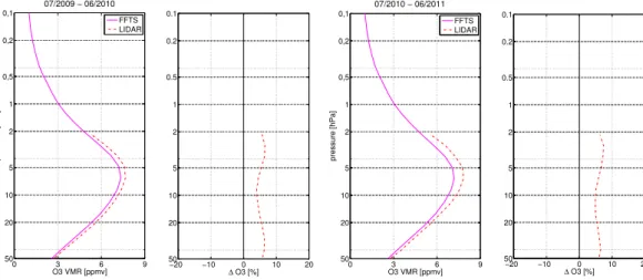
Annual mean ozone profiles from GROMOS FFTS and OHP lidar are presented in Fig. 2. The averaged time period is July 2009 to June 2010 (left-hand side) and July 5

2010 to June 2011 (right-hand side). Two annual means are shown to see if there is a possible difference between the years. Volume mixing ratios are plotted against at-mospheric pressure. Lidar profiles have been convolved with the averaging kernels of GROMOS (Eq. 1). The averaged ozone profiles of GROMOS FFTS are shown in ma-genta and lidar profiles are given by the red dashed-dotted curves. The lidar measures 10

up to ∼ 2 hPa. Also given to the right of the mean profiles in Fig. 2 are the mean relative difference profiles ∆O_3,rel as defined by Eq. (2).

In both annual mean profiles, GROMOS FFTS and lidar show good agreement with GROMOS FFTS measuring slightly less ozone values compared to the lidar. The an-nual mean relative differences ∆O_3,rel for both time periods are between+3 and +8 % 15

in the 50 to 2 hPa region (about 22 to 44 km). Note that the two annual mean difference profiles show a similar structure and no large differences are evident between the two years.

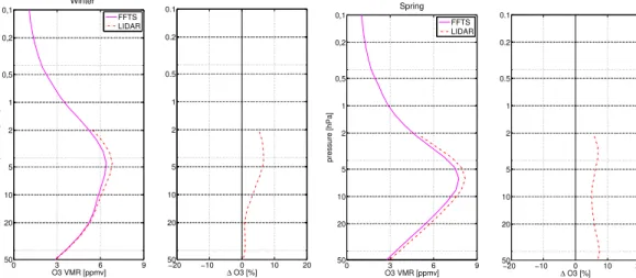
5.1.2 Seasonal mean

Seasonal differences between GROMOS FFTS and lidar could have been smoothed 20

out when calculating the annual mean profiles. Therefore, we investigate the existence of possible seasonal biases by looking at the mean seasonal profiles. Figures 3 and 4 show the mean profiles as well as the mean difference profiles from two years (2010 and 2011) for winter (December to February), spring (March to May), summer (June to August) and autumn (September to November). Clearly visible are the higher ozone 25

(17)

AMTD

Full Screen / Esc

values of both instruments in summer compared to winter (8 ppm, respectively 6 ppm). Looking at the mean difference profiles of spring and autumn, we find them to be quite constant with altitude. While for summer, relative mean differences ∆O_3,rel are largest below 20 hPa, the largest difference in winter is found around ozone peak height at 5 hPa. This larger difference in the middle stratosphere of winter can be due to the 5

different measurement locations. The stratospheric ozone layer in winter is more dis-turbed than in summer due to high wave activity. In addition, strong horizontal gradients of ozone are present during winter when Bern and OHP are close to the polar vortex edge.

Overall, no seasonal biases are evident and relative mean differences ∆O_3,rel be-10

tween GROMOS FFTS and lidar are below 8 %.

5.2 Satellites, ERA-interim and ozonesondes

5.2.1 Annual mean

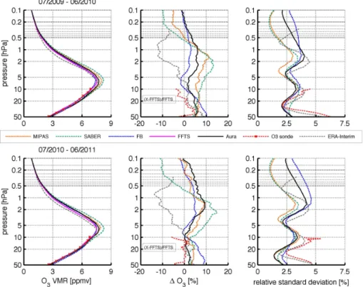
A comparison of annual mean profiles between GROMOS FFTS, GROMOS FB, satel-lites, ozonesondes and ERA-Interim is shown in Fig. 5. Again, two annual averages 15

are calculated: top panels shows the time period July 2009 to June 2010 and bottom panels show July 2010 to June 2011. The left panels give annual mean volume mixing ratio profiles. The mean relative difference profiles ∆O_3,rel(Eq. 2) are shown in the mid-dle panels and the relative standard deviations can be found in the right panels. The data from satellite-borne instruments, ozonesonde and ERA-Interim profiles have been 20

convolved with AVK from GROMOS FFTS to account for their higher vertical resolu-tion (see Sect. 4.2). No AVK smoothing has been applied to the GROMOS FB profiles which have a vertical resolution comparable to GROMOS FFTS and similar a priori ozone profiles.

MIPAS is given by the orange lines, SABER in green dashed, GROMOS FB is given 25

(18)

AMTD

Full Screen / Esc

black line, ozonesondes in red dashed and finally ERA-Interim can be found in grey dashed.

The general agreement is within 10 % between 50 and 0.1 hPa. Exceptions are SABER around 2 hPa and ERA-Interim above 3 hPa. The large difference between GROMOS FFTS and SABER can be explained by a previously reported, systematic 5

high bias of 10–20 % for SABER’s ozone values from the middle stratosphere to the lower mesosphere (Rong et al., 2009).

ERA-Interim and GROMOS FFTS agree well up to 3 hPa and the mean relative dif-ference ∆O_3,rel is ±5 %, while above ERA-Interim has about 10 % less ozone. The oscillatory nature of the relative standard deviations is a noticeable feature and visible 10

in all data sets. Generally, GROMOS FFTS ozone profiles shows a slight negative bias of a few percent compared to the other data in the 50 to 0.1 hPa region. The two annual means show a consistent picture and no large differences can be found between the annual means of July 2009–June 2010 and July 2010–June 2011.

5.2.2 Seasonal mean

15

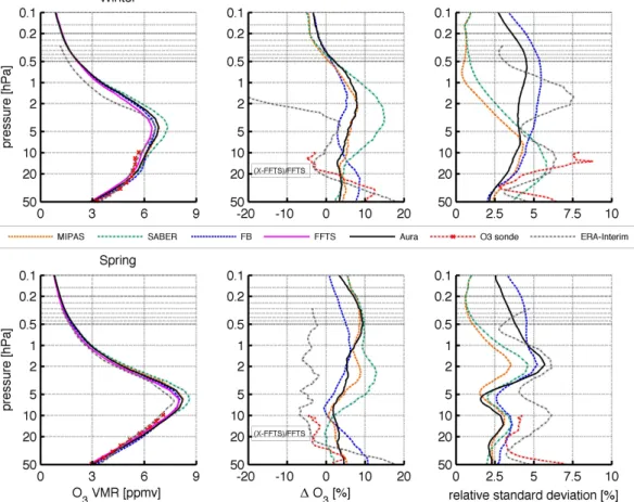
To detect a possible seasonal bias, we look again at the seasonal mean profiles of the years 2010 and 2011 by summing the months of December to February (winter), the months of March to May (spring), the months of June to August (summer) and the months of September to November (autumn). The results can be found in Fig. 6a (winter and spring) and Fig. 6b (summer and autumn). The mean ozone profiles are 20

given in the left panels. The mean relative differences can be found in the middle panels and the right panels show the relative standard deviations of all data sets. The color code is the same as in the comparison of annual mean profiles of Fig. 5. For winter, we find indication for a double peak structure in all ozone profiles. The comparisons confirm the results of the previous Sect. 5.1. Namely, that ozone values from GROMOS 25

FFTS are slightly lower than those from the external instruments. Looking at the mean relative differences of Fig. 6a and b, we find a consistent picture with similar difference profiles for all seasons. An exception is ERA-Interim: in the winter upper stratosphere,

(19)

AMTD

Full Screen / Esc

mean relative differences are up to −25 %, while they are mostly within ±10 % for the other seasons. This strong winter deviation may be partly explained since accurate modelling of the stratospheric ERA-Interim ozone field at high latitudes is difficult during winter (Dragani, 2011).

Please note the larger standard deviations in the winter stratosphere (around 5 %) 5

compared to summer (around 2 %). In winter, the stratosphere is more disturbed due to higher planetary wave activity than in summer, when the atmosphere is more stable. This can also be seen in the mean relative difference profile ∆O_3,relof GROMOS FFTS and ozonesonde. We find that the agreement for summer is better (around 4 %) than for winter (up to 12 %). As mentioned in Sect. 5.1.2, in winter, collocation might be more 10

critical than in summer, since during winter months the polar vortex is often shifted toward midlatitudes and strong horizontal ozone gradients occur.

6 Comparison of ozone time series

6.1 GROMOS and lidar

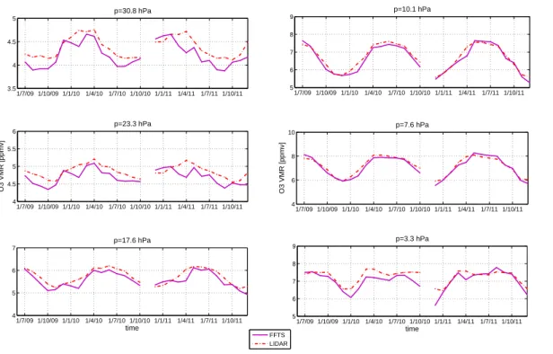
Figure 7 displays the monthly mean time series of coinciding GROMOS FFTS (ma-15

genta line) and lidar (red dashed-dotted line) measurements for six pressure levels. Lidar profiles have been convolved with GROMOS FFTS averaging kernels. The data gap in November 2010 is due to missing lidar data during that month. GROMOS FFTS and lidar generally agree well at all pressure levels. Clearly visible is the strong annual variation in the stratosphere with maximal ozone values during summer months. The 20

largest difference between GROMOS FFTS and lidar is found in the lower stratosphere at 31 hPa.

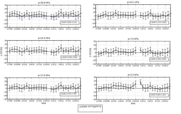
Monthly mean relative differences ((LIDAR-FFTS)/FFTS) are depicted in Fig. 8. Pres-sure levels are the same as in Fig. 7. Error bars are standard deviation of the averaged data. The mean relative difference is less than 10 % for all pressure levels shown. The 25

(20)

AMTD

Full Screen / Esc

in the lower right corner for each pressure level. A maximum value of+3.8 % at 31 hPa and a minimum value of+1.4 % at 7.6 hPa is found.

6.2 GROMOS, satellites and ERA-Interim

The time series of GROMOS and ozone data from satellite-borne instruments as well as ERA-Interim are shown in Fig. 9a to c. They display the monthly mean ozone val-5

ues of collocated measurements on fixed pressure levels for the time period July 2009 to December 2011. Figure 9a shows lower mesospheric ozone, while Fig. 9b depicts middle stratospheric ozone and Fig. 9c the lower stratospheric ozone. Colors are the same as in the mean profiles of Sect. 5.2. MIPAS time series are only shown for alti-tudes at 1.1 hPa and below. Since only a few ACE-FTS profiles have been found for the 10

selection criteria applied, no averaging could be performed and single profile values for the given pressure levels are shown as grey squares.

The time series agree well at all altitudes. Some features are pointed out: (1) at 0.1 hPa, GROMOS FFTS values are larger than the other instruments during sum-mer and smaller during winter, (2) ERA-Interim ozone clearly is underestimating ozone 15

above 3.3 hPa and has no annual cycle in contrast to all other instruments, (3) at 23 hPa, the largest differences can be found for GROMOS FFTS and GROMOS FB, while the satellite instruments cover the ozone VMR range in between.

Generally, GROMOS FFTS always measures at the lower edge of the range of ozone values in all time series. This slight low bias of a few percent was already seen when 20

looking at the mean profiles in Sect. 5. The bias of GROMOS FFTS in the stratosphere, Fig. 9b and c, appears to slightly improve with time and might be due to instrumental issues after adding the new FFTS backend in July 2009. Please also note the clear annual cycle, which shifts from winter maximum in the lower mesosphere to summer maximum in the stratosphere. The strongest annual variation is observed at 10 hPa 25

(21)

AMTD

Full Screen / Esc

6.3 A closer look on GROMOS and Aura/MLS

Time series of percent differences between collocated GROMOS FFTS and Aura/MLS ozone profiles are displayed in Fig. 10a to c. The relative differences are calculated according to Eq. (2) and shown are the same pressure levels as used in Sect. 6.2. The shaded grey area gives the relative mean standard deviation. The agreement is 5

generally within 10 % and improves with time.

In the stratosphere, the largest difference between GROMOS and Aura/MLS can be found in winter 2009/2010. A minor sudden stratospheric warming (SSW) occurred in December 2009, followed by major SSW event in January 2010 (Kuttippurath and Nikulin, 2012). The larger variability associated with the disturbed winter stratosphere 10

is also indicated by the larger standard deviation.

The mean relative difference for the whole time period is given in the lower right cor-ners at each pressure level. The maximum is found at 0.6 hPa with a mean difference of +6.9 %, while the minimum is found around at 17.6 hPa (around ozone volume mixing ratio peak height) with a value of+3.2 %.

15

A scatter plot of coincident ozone measurements of Aura/MLS and GROMOS FFTS for fixed pressure levels is given in Fig. 11. The black dashed-dotted line indicates 1-1, representing ideal agreement. The magenta line is the best fit straight line. The lines agree well for for pressure levels from 30.8 to 0.6 hPa. The correlation coefficients are given in the lower right corner for each pressure level. Good correlation is found for 20

all altitudes. A maximum correlation of R= 0.95 is found at 10 hPa. At 0.1 hPa, the correlation is minimal with R= 0.64.

6.4 Dynamics in the stratosphere

Daily mean time series of ozone between 100 and 0.1 hPa and from July 2009 to December 2011 are shown in Fig. 12. Top to bottom shows GROMOS FFTS, GROMOS 25

FB, and collocated MLS, MIPAS, SABER and ERA-Interim reanalysis. No smoothing with GROMOS AVK has been applied to the satellite and ERA-Interim ozone profiles.

(22)

AMTD

Full Screen / Esc

The annual cycle can be clearly seen in all ozone data sets with stratospheric ozone values around 8 ppm (red) in summer and around 6 ppm (yellow) in winter. Similar structures in ozone variability are found in all time series, particularly when one looks at the winter periods of 2009/2010 and 2010/2011. The winter stratosphere is strongly disturbed since wave activity is larger in winter than in summer (Tsuda et al., 2000; 5

Alexander and Shepherd, 2010). All ozone time series show strong decrease and in-crease of ozone values over the course of a few weeks and exhibit signatures of atmo-spheric waves. These wave-like perturbation in ozone occur simultaneously and with similar amplitudes in all six time series. A major sudden stratospheric warming (SSW) occurred in the Northern Hemisphere in January 2010 and led to a depletion of ozone. 10

More details on the ozone distribution during SSW events can be found e.g. in Flury et al. (2009), Scheiben et al. (2012) and Goncharenko et al. (2012)

7 Conclusions

The GROund-based Millimeter-wave Ozone Spectrometer GROMOS is a 142 GHz ground-based radiometer which has been upgraded in July 2009 by a new Fast-Fourier 15

Transform spectrometer (FFTS). To assess the quality of the ozone profiles retrieved from the high-resolution ozone line spectra of the FFTS, we compare ozone profiles from the FFTS with results from the original filter bench (FB) backend. The time period studied is July 2009 to December 2011.

Further, an intercomparison for the same time period is carried out by using 20

other, independent data sets. These include collocated satellite data (MIPAS/ENVISAT, MLS/Aura, SABER/TIMED, ACE-FTS/SCISAT-1), lidar measurements from the Obser-vatoire Haute Provence (OHP), ozonesondes profiles from Payerne and the ERA-Interim ozone data product.

We find that GROMOS FFTS and GROMOS FB ozone profiles agree within 5 % 25

between 20 and 0.1 hPa. A homogenization between the GROMOS FB and GROMOS FFTS time series will be realized by taking the FFTS as benchmark for the FB. The

(23)

AMTD

Full Screen / Esc

mean difference between external instruments (satellite and lidar) and GROMOS FFTS was found to be within 10 % for the 50 to 0.1 hPa region. Over the whole time period July 2009 to December 2011, the average mean difference between GROMOS FFTS and lidar was maximal with+3.8 % at 31 hPa and minimal with +1.4 % at 7.6 hPa. A closer look at the time series from GROMOS FFTS and Aura/MLS show very good correlation 5

on all pressure levels. Correlation coefficients range from R = 0.64 at 0.1 hPa (lowest correlation) to R= 0.95 at 10 hPa (highest correlation). The overall agreement between GROMOS FFTS and Aura/MLS is within 5 % in the stratosphere.

GROMOS is thus well suited to provide local information about ozone changes on intraseasonal and seasonal time scales. Due to the high time resolution of 30 min, the 10

data set of GROMOS enables us to study short-term ozone variations in the atmo-sphere such as e.g. the diurnal cycle in stratospheric ozone. After merging GROMOS FB and FFTS, we will be able to address changes in the ozone distribution above Switzerland over nearly two decades.

Acknowledgements. Simone Studer is funded by the Swiss National Science Foundation SNF

15

under grant no. 200020-134613. The work was further supported by the EU project NORS (FP7-SPACE-2011-284421) and the International Space Science Institute (http://www.issibern. ch/teams/ozonetrend/). We thank the MLS- and SABER-team for the ozone data used in this study which was retrieved from the NASA Goddard Space Flight Center, the MIPAS-team from Karlsruhe Institute of Technology (KIT) for provision of MIPAS ozone data. The

ACE-20

FTS/SCISAT-1 ozone profiles are mainly supported by the Canadian Space Agency and the Natural Sciences and Engineering Research Council of Canada. The author would further like to thank MeteoSwiss for providing us with ozonesonde data from Payerne.

(24)

AMTD

Full Screen / Esc

Printer-friendly Version Interactive Discussion Discussion P a per | D iscussion P a per | Discussion P a per | Discuss ion P a per | References

Adams, C., Strong, K., Batchelor, R. L., Bernath, P. F., Brohede, S., Boone, C., Degenstein, D., Daffer, W. H., Drummond, J. R., Fogal, P. F., Farahani, E., Fayt, C., Fraser, A., Goutail, F., Hendrick, F., Kolonjari, F., Lindenmaier, R., Manney, G., McElroy, C. T., McLinden, C. A., Mendonca, J., Park, J.-H., Pavlovic, B., Pazmino, A., Roth, C., Savastiouk, V., Walker, K. A.,

5

Weaver, D., and Zhao, X.: Validation of ACE and OSIRIS ozone and NO₂ measurements

using ground-based instruments at 80◦N, Atmos. Meas. Tech., 5, 927–953,

doi:10.5194/amt-5-927-2012, 2012. 6107

Alexander, S. P. and Shepherd, M. G.: Planetary wave activity in the polar lower stratosphere, Atmos. Chem. Phys., 10, 707–718, doi:10.5194/acp-10-707-2010, 2010. 6117

10

Antón, M., López, M., Vilaplana, J. M., Kroon, M., McPeters, R., Bañón, M., and Ser-rano, A.: Validation of OMI-TOMS and OMI-DOAS total ozone column using five Brewer spectroradiometers at the Iberian peninsula, J. Geophys. Res.-Atmos., 114, D14307, doi:10.1029/2009JD012003, 2009. 6099

Bernath, P. F., McElroy, C. T., Abrams, M. C., Boone, C. D., Butler, M., Camy-Peyret, C.,

Car-15

leer, M., Clerbaux, C., Coheur, P.-F., Colin, R., DeCola, P., DeMaziBernath, P. F., McEl-roy, C. T., Abrams, M. C., Boone, C. D., Butler, M., Camy-Peyret, C., Carleer, M., Cler-baux, C., Coheur, P.-F., Colin, R., DeCola, P., DeMaziere, M., Drummond, J. R., Dufour, D., Evans, W. F. J., Fast, H., Fussen, D., Gilbert, K., Jennings, D. E., Llewellyn, E. J., Lowe, R. P., Mahieu, E., McConnell, J. C., McHugh, M., McLeod, S. D., Michaud, R., Midwinter, C.,

20

Nassar, R., Nichitiu, F., Nowlan, C., Rinsland, C. P., Rochon, Y. J., Rowlands, N., Seme-niuk, K., Simon, P., Skelton, R., Sloan, J. J., Soucy, M.-A., Strong, K., Tremblay, P., Turn-bull, D., Walker, K. A., Walkty, I., Wardle, D. A., Wehrle, V., Zander, R., and Zou, J.: Atmo-spheric Chemistry Experiment (ACE): mission overview, Geophys. Res. Lett., 32, L15S01, doi:10.1029/2005GL022386, 2005. 6107

25

Bleisch, R., Kämpfer, N., and Haefele, A.: Retrieval of tropospheric water vapour by using spec-tra of a 22 GHz radiometer, Atmos. Meas. Tech., 4, 1891–1903, doi:10.5194/amt-4-1891-2011, 2011. 6109

Calisesi, Y.: The Stratospheric Ozone MOnitoring RAdiometer SOMORA: NDSC Appli-cation Document, IAP Research report, University of Bern, Bern, Switzerland, 11,

30

(25)

AMTD

Full Screen / Esc

Calisesi, Y., Peter, R., Kaempfer, N., and Stuebli, R.: Intercomparison of ozone profiles by radiosoundings over Payerne and microwave measurements in Bern: updated report, Re-search Report 98-9, Institut für angewandte Physik, Universität Bern, Bern, Switzerland, 1998. 6108

Calisesi, Y., Werli, H., and Kaempfer, N.: Midstratospheric ozone variability over Bern related to

5

planetary wave activity during the winters 1994–1995 to 1998–1999, J. Geophys. Res., 106, 7903–7916, 2001. 6101

Chubachi, S.: A special ozone observation at syowa station, antarctica from February 1982 to January 1983, in: Atmospheric Ozone, edited by: Zerefos, C. and Ghazi, A., Springer Netherlands, 10.1007/978-94-009-5313-0_58, 285–289, 1985. 6099

10

Dee, D. P., Uppala, S. M., Simmons, A. J., Berrisford, P., Poli, P., Kobayashi, S., Andrae, U., Balmaseda, M. A., Balsamo, G., Bauer, P., Bechtold, P., Beljaars, A. C. M., van de Berg, L., Bidlot, J., Bormann, N., Delsol, C., Dragani, R., Fuentes, M., Geer, A. J., Haimberger, L., Healy, S. B., Hersbach, H., Hólm, E. V., Isaksen, L., Kållberg, P., Köhler, M., Matricardi, M., McNally, A. P., Monge-Sanz, B. M., Morcrette, J.-J., Park, B.-K., Peubey, C., de Rosnay, P.,

15

Tavolato, C., Thépaut, J.-N., and Vitart, F.: The ERA-Interim reanalysis: configuration and performance of the data assimilation system, Q. J. Roy. Meteorol. Soc., 137, 553–597, doi:10.1002/qj.828, 2011. 6107

Dragani, R.: On the quality of the ERA-Interim ozone reanalyses: comparison with satellite data, Q. J. Roy. Meteorol. Soc., 137, 1312–1326, doi:10.5194/amt-5-927-2012, 2011. 6107,

20

6114

Dumitru, M. C., Hocke, K., Kaempfer, N., and Calisesi, Y.: Comparison and validation studies related to ground-based microwave observations of ozone in the stratosphere and meso-sphere, J. Atmos. Sol.-Terr. Phy., 68, 745–756, 2006. 6101, 6115

Dupuy, E., Walker, K. A., Kar, J., Boone, C. D., McElroy, C. T., Bernath, P. F., Drummond, J. R.,

25

Skelton, R., McLeod, S. D., Hughes, R. C., Nowlan, C. R., Dufour, D. G., Zou, J., Nichitiu, F., Strong, K., Baron, P., Bevilacqua, R. M., Blumenstock, T., Bodeker, G. E., Borsdorff, T., Bourassa, A. E., Bovensmann, H., Boyd, I. S., Bracher, A., Brogniez, C., Burrows, J. P., Catoire, V., Ceccherini, S., Chabrillat, S., Christensen, T., Coffey, M. T., Cortesi, U., Davies, J., De Clercq, C., Degenstein, D. A., De Mazière, M., Demoulin, P., Dodion, J., Firanski, B.,

Fis-30

cher, H., Forbes, G., Froidevaux, L., Fussen, D., Gerard, P., Godin-Beekmann, S., Goutail, F., Granville, J., Griffith, D., Haley, C. S., Hannigan, J. W., Höpfner, M., Jin, J. J., Jones, A., Jones, N. B., Jucks, K., Kagawa, A., Kasai, Y., Kerzenmacher, T. E., Kleinböhl, A.,

(26)

Kleko-AMTD

Full Screen / Esc

ciuk, A. R., Kramer, I., Küllmann, H., Kuttippurath, J., Kyrölä, E., Lambert, J.-C., Livesey, N. J., Llewellyn, E. J., Lloyd, N. D., Mahieu, E., Manney, G. L., Marshall, B. T., McConnell, J. C., Mc-Cormick, M. P., McDermid, I. S., McHugh, M., McLinden, C. A., Mellqvist, J., Mizutani, K., Mu-rayama, Y., Murtagh, D. P., Oelhaf, H., Parrish, A., Petelina, S. V., Piccolo, C., Pommereau, J.-P., Randall, C. E., Robert, C., Roth, C., Schneider, M., Senten, C., Steck, T., Strandberg, A.,

5

Strawbridge, K. B., Sussmann, R., Swart, D. P. J., Tarasick, D. W., Taylor, J. R., Tétard, C., Thomason, L. W., Thompson, A. M., Tully, M. B., Urban, J., Vanhellemont, F., Vigouroux, C.,

von Clarmann, T., von der Gathen, P., von Savigny, C., Waters, J. W., Witte, J. C., Wolff, M.,

and Zawodny, J. M.: Validation of ozone measurements from the Atmospheric Chemistry Experiment (ACE), Atmos. Chem. Phys., 9, 287–343, doi:10.5194/acp-9-287-2009, 2009.

10

6107

Eriksson, P., Jiménez, C., and Buehler, S. A.: Qpack, a general tool for instrument simula-tion and retrieval work, J. Quant. Spectrosc. Ra., 91, 47–64, doi:10.1016/j.jqsrt.2004.05.050, 2005. 6102

Eriksson, P., Buehler, S. A., Davis, C. P., Emde, C., and Lemke, O.: ARTS, the

atmo-15

spheric radiative transfer simulator, Version 2, J. Quant. Spectrosc. Ra., 112, 1551–1558, doi:10.1016/j.jqsrt.2011.03.001, 2011. 6102

Farman, J. C., Gardiner, B. G., and Shanklin, J. D.: Large losses of total ozone in Antarctica

reveal seasonal ClO_x/NO_x interaction, Nature, 315, 207–210, doi:10.1038/315207a0, 1985.

6099

20

Fischer, H., Birk, M., Blom, C., Carli, B., Carlotti, M., von Clarmann, T., Delbouille, L., Dud-hia, A., Ehhalt, D., Endemann, M., Flaud, J. M., Gessner, R., Kleinert, A., Koopman, R., Langen, J., López-Puertas, M., Mosner, P., Nett, H., Oelhaf, H., Perron, G., Remedios, J., Ridolfi, M., Stiller, G., and Zander, R.: MIPAS: an instrument for atmospheric and climate research, Atmos. Chem. Phys., 8, 2151–2188, doi:10.5194/acp-8-2151-2008, 2008. 6105

25

Flury, T., Hocke, K., Haefele, A., Kämpfer, N., and Lehmann, R.: Ozone depletion, water vapor increase, and PSC generation at midlatitudes by the 2008 major stratospheric warming, J. Geophys. Res., 114, D18302, doi:10.1029/2009JD011940, 2009. 6101, 6117

Froidevaux, L., Jiang, Y. B., Lambert, A., Livesey, N. J., Read, W. G., Waters, J. W., Brow-ell, E. V., Hair, J. W., Avery, M. A., McGee, T. J., Twigg, L. W., Sumnicht, G. K., Jucks, K. W.,

30

Margitan, J. J., Sen, B., Stachnik, R. A., Toon, G. C., Bernath, P. F., Boone, C. D., Walker, K. A., Filipiak, M. J., Harwood, R. S., Fuller, R. A., Manney, G. L., Schwartz, M. J.,

(27)

Pe-AMTD

Full Screen / Esc

run, V. S., Snyder, W. V., Stek, P. C., Thurstans, R. P., and Wagner, P. A.: Validation of Aura Mi-crowave Limb Sounder stratospheric ozone measurements, J. Geophys. Res.-Atmos., 113, D15S20, doi:10.1029/2007JD008771, 2008. 6106

Gebhardt, C., Rozanov, A., Hommel, R., Weber, M., Bovensmann, H., Burrows, J. P., Degen-stein, D., Froidevaux, L., and Thompson, A. M.: Stratospheric ozone trends and variability

5

as seen by SCIAMACHY during the last decade, Atmos. Chem. Phys. Discuss., 13, 11269– 11313, doi:10.5194/acpd-13-11269-2013, 2013. 6099

Godin, S., Carswell, A. I., Donovan, D. P., Claude, H., Steinbrecht, W., McDermid, I. S.,

McGee, T. J., Gross, M. R., Nakane, H., Swart, D. P. J., Bergwerff, H. B., Uchino, O., von der

Gathen, P., and Neuber, R.: Ozone Differential Absorption Lidar Algorithm Intercomparison,

10

Appl. Optics, 38, 6225–6236, doi:10.1364/AO.38.006225, 1999. 6105

Godin-Beekmann, S. and Nair, P. J.: Sensitivity of stratospheric ozone lidar measurements to a change in ozone absorption cross-sections, J. Quant. Spectrosc. Ra., 113, 1317–1321, doi:10.1016/j.jqsrt.2012.03.002, 2012. 6105

Godin-Beekmann, S., Porteneuve, J., and Garnier, A.: Systematic DIAL lidar monitoring of

15

the stratospheric ozone vertical distribution at Observatoire de Haute-Provence (43.92◦N,

5.71◦E), J. Environ. Monitor., 5, 57–67, 2003. 6104, 6105

Goncharenko, L. P., Coster, A. J., Plumb, R. A., and Domeisen, D. I. V.: The potential role of stratospheric ozone in the stratosphere-ionosphere coupling during stratospheric warmings, Geophys. Res. Lett., 39, L08101, doi:10.1029/2012GL051261, 2012. 6117

20

Harris, N. R. P., Kyrö, E., Staehelin, J., Brunner, D., Andersen, S.-B., Godin-Beekmann, S., Dhomse, S., Hadjinicolaou, P., Hansen, G., Isaksen, I., Jrrar, A., Karpetchko, A., Kivi, R., Knudsen, B., Krizan, P., Lastovicka, J., Maeder, J., Orsolini, Y., Pyle, J. A., Rex, M., Van-icek, K., Weber, M., Wohltmann, I., Zanis, P., and Zerefos, C.: Ozone trends at north-ern mid- and high latitudes – a European perspective, Ann. Geophys., 26, 1207–1220,

25

doi:10.5194/angeo-26-1207-2008, 2008. 6099

Hocke, K., Kämpfer, N., Feist, D. G., Calisesi, Y., Jiang, J. H., and Chabrillat, S.: Temporal variance of lower mesospheric ozone over Switzerland during winter 2000/2001, Geophys. Res. Lett., 33, L09801, doi:10.1029/2005GL025496, 2006. 6101, 6107

Hocke, K., Kämpfer, N., Ruffieux, D., Froidevaux, L., Parrish, A., Boyd, I., von Clarmann, T.,

30

Steck, T., Timofeyev, Y. M., Polyakov, A. V., and Kyrölä, E.: Comparison and synergy of strato-spheric ozone measurements by satellite limb sounders and the ground-based microwave

(28)

AMTD

Full Screen / Esc

radiometer SOMORA, Atmos. Chem. Phys., 7, 4117–4131, doi:10.5194/acp-7-4117-2007, 2007. 6101

Hocke, K., Studer, S., Martius, O., Scheiben, D., and Kämpfer, N.: A 20-day period standing oscillation in the northern winter stratosphere, Ann. Geophys., 31, 755–764, doi:10.5194/angeo-31-755-2013, 2013. 6101

5

Ingold, T., Peter, R., and Kämpfer, N.: Weighted mean tropospheric temperature and transmit-tance determination at milimeter-wave frequencies for ground-based application, Radio Sci., 33, 905–918, 1998. 6101, 6103

Jiang, Y. B., Froidevaux, L., Lambert, A., Livesey, N. J., Read, W. G., Waters, J. W., Bo-jkov, B., Leblanc, T., McDermid, I. S., Godin-Beekmann, S., Filipiak, M. J., Harwood, R. S.,

10

Fuller, R. A., Daffer, W. H., Drouin, B. J., Cofield, R. E., Cuddy, D. T., Jarnot, R. F., Knosp, B. W., Perun, V. S., Schwartz, M. J., Snyder, W. V., Stek, P. C., Thurstans, R. P., Wagner, P. A., Allaart, M., Andersen, S. B., Bodeker, G., Calpini, B., Claude, H., Coetzee, G., Davies, J., De Backer, H., Dier, H., Fujiwara, M., Johnson, B., Kelder, H., Leme, N. P., König-Langlo, G., Kyro, E., Laneve, G., Fook, L. S., Merrill, J., Morris, G., Newchurch, M.,

15

Oltmans, S., Parrondos, M. C., Posny, F., Schmidlin, F., Skrivankova, P., Stubi, R., Tara-sick, D., Thompson, A., Thouret, V., Viatte, P., Vömel, H., von Der Gathen, P., Yela, M., and Zablocki, G.: Validation of Aura Microwave Limb Sounder Ozone by ozonesonde and lidar measurements, J. Geophys. Res.-Atmos., 112, D24S34, doi:10.1029/2007JD008776, 2007. 6106

20

Kramarova, N. A., Frith, S. M., Bhartia, P. K., McPeters, R. D., Taylor, S. L., Fisher, B. L., Labow, G. J., and DeLand, M. T.: Validation of ozone monthly zonal mean profiles obtained from the Version 8.6 Solar Backscatter Ultraviolet algorithm, Atmos. Chem. Phys. Discuss., 13, 2549–2597, doi:10.5194/acpd-13-2549-2013, 2013. 6099

Kuntz, M.: A new implementation of the Humlicek algorithm for the calculation of the Voigt

25

profile function, J. Quant. Spectrosc. Ra., 57, 819–824, doi:10.1016/S0022-4073(96)00162-8, 1997. 6103

Kuttippurath, J. and Nikulin, G.: A comparative study of the major sudden stratospheric warm-ings in the Arctic winters 2003/2004–2009/2010, Atmos. Chem. Phys., 12, 8115–8129, doi:10.5194/acp-12-8115-2012, 2012. 6116

30

Laeng, A., Grabowski, U., Clarmann, T. V., Stiller, G., Kellmann, S., Kiefer, M., Linden, A., Los-sow, S., Bathgate, T., Bernath, P., Boone, C. D., Clerbaux, C., Degenstein, D., Fritz, S., Froide-vaux, L., Hervig, M., Hoppel, K., Lumpe, J., McHugh, M., Sano, T., Sofieva, V., Suzuki, M.,

(29)

AMTD

Full Screen / Esc

Tamminen, J., Urban, J., Walker, K., Weber, M., and Zawodny, J.: Validation of MIPAS IMK/IAA ozone profiles, in: Quadrennial Ozone Symposium, Toronto, 2012. 6105

Lobsiger, E.: Ground-based microwave radiometry to determine stratospheric and mesospheric ozone profiles, J. Atmos. Terr. Phys., 49, 493–501, 1987. 6101

Lobsiger, E., Künzi, K. F., and Dütsch, H. U.: Comparison of stratospheric ozone profiles

re-5

trieved from microwave-radiometer and Dobson-spectrometer data, J. Atmos. Terr. Phys., 46, 799–806, 1984. 6101

Maillard Barras, E., Ruffieux, D., and Hocke, K.: Stratospheric ozone profiles over Switzerland

measured by SOMORA, ozonesonde and MLS/AURA satellite, Int. J. Remote Sens., 30, 4033–4041, 2009. 6107

10

McLinden, C. A. and Fioletov, V.: Quantifying stratospheric ozone trends: complications due to stratospheric cooling, Geophys. Res. Lett., 38, L03808, doi:10.1029/2010GL046012, 2011. 6099

Müller, S., Murk, A., Monstein, C., and Kämpfer, N.: Intercomparison of digital fast fourier trans-form and acoustooptical spectrometers for microwave radiometry of the atmosphere, IEEE

15

T. Geosci. Remote, 47, 2233–2239, doi:10.1109/TGRS.2009.2013695, 2009. 6101

Nair, P. J., Godin-Beekmann, S., Pazmiño, A., Hauchecorne, A., Ancellet, G.,

Petropavlovskikh, I., Flynn, L. E., and Froidevaux, L.: Coherence of long-term stratospheric ozone vertical distribution time series used for the study of ozone recovery at a northern mid-latitude station, Atmos. Chem. Phys., 11, 4957–4975, doi:10.5194/acp-11-4957-2011,

20

2011. 6105

Nair, P. J., Godin-Beekmann, S., Kuttippurath, J., Ancellet, G., Goutail, F., Pazmiño, A., Froide-vaux, L., Zawodny, J. M., Evans, R. D., and Pastel, M.: Ozone trends derived from the total column and vertical profiles at a northern mid-latitude station, Atmos. Chem. Phys. Discuss., 13, 7081–7112, doi:10.5194/acpd-13-7081-2013, 2013. 6099

25

Peter, R.: The ground-based millimeter-wave ozone spectrometer-GROMOS, IAP Research Report, University of Bern, Bern, Switzerland, 13, 1997. 6103

Peter, R. and Kämpfer, N.: Short-term variations of mid-latitude ozone profiles during the winter

1994/95, in: Proc. Third Europ. Symp. on Polar O₃Res., Air Pollution Res. Rep. No. 56 of the

EC, September 1995, Schliersee, Germany, 484–487, 1995. 6101

30

Peter, R., Caliseri, Y., and Kämpfer, N.: Variability of middle atmospheric ozone abundances derived from continuous ground-based millimeter wave measurements, in: Proceedings of the XVIII Quadrennial Ozone Symposium, 12–21 September 1996, L’Aquila, Italy, edited by: