ENERGY LABORATORY DATA AND MODEL DIRECTORY
S. Lahiri Editors: J. Carson
MIT Energy Laboratory Report No. MIT-EL 81-025 July 1981
MITLibraries
Document Services Room 14-0551 77 Massachusetts Avenue Cambridge, MA 02139 Ph: 617.253.5668 Fax: 617.253.1690 Email: docs@mit.edu http://libraries.mit.edu/docsDISCLAIMER OF QUALITY
Due to the condition of the original material, there are unavoidable flaws in this reproduction. We have made every effort possible to
provide you with the best copy available. If you are dissatisfied with this product and find it unusable, please contact Document Services as
soon as possible. Thank you.
Pgs. 113,150, 151,
&
159 are missing from the archival
copy. This is the most complete version available.
Table of Contents
Page
I. COMPLETED RESEARCH MODELS AND ASSOCIATED DATA COLLECTIONS
1. Regionalized Electricity Model 1
2. Econometric Policy Model of Natural Gas 24
3. Coal Policy Model 43
II. CURRENT-ACTIVE MODELS AND ASSOCIATED DATA COLLECTIONS
1. Industrial Energy Demand Model 56
2. M.I.T. Energy Laboratory Energy Macro Model 60
3. Integrated Coal Analysis Model 62
4. Electric Utility System Generation 70
5. Analytical Models of the World Oil Market 73 III. DEVELOPING MODELS AND ASSOCIATED DATA COLLECTIONS
1. Electricity Generation Expansion Analysis System 111
2. Residential Energy Demand Model 118
3. Optional Energy System Simulator 130
4. Probabilistic Oil Discovery Model 135
5. Macro-Economic Model of Venezuela 138
6. Solar Energy Flux Computation 139
7. Utility Financial/Regulatory Analysis Model 146 8. Electricity Rate-Setting Model (ERATES) 148
9. Photovoltaic 1 151
IV. FREE-STANDING DATA COLLECTIONS
1. Energy Macro Data Base 157
2. Interfuel Substitution 160
3. SOLOPS 161
4. SOLMET (National Climatic Center) 164
5. Energy Model Data Base (Brookhaven National Laboratory) 166
V. APPENDIX: RESPONSE FORM "lc--- - -1=wMll wM1l--3
FOREWORD
Over the past several years M.I.T. faculty, staff, and students have produced a substantial body of research and analysis relating to the production, conversion, and use of energy in domestic and inter-national markets. Much of this research takes the form of models and associated data bases that have enduring value in policy studies
(models) and in supporting related research and modeling efforts (data). For such models and data it is important to ensure that the useful life cycle does not end with the conclusion of the research project.
In an effort to develop a mechanism for supporting the maintenance and appropriate access to Energy Laboratory associated models and data, the Laboratory's Center for Energy Policy Research (CEPR) has sponsored a project to prepare this Energy Laboratory Data and Model Directory, edited by Dr. Supriya Lahiri and Ms. Jacqueline Carson. The Directory provides a survey of selected models and data bases and includes
descriptive information, current status, mode of access, and contact persons. This directory represents the conclusion of this project.
This directory is an important step in extending the usefulness of models and data bases available here at the M.I.T. Energy Laboratory. It will be updated from time to time to include new models and data bases that have been developed, or significant changes that have occurred in the entries included here. You suggestions and comments are welcome.
David 0. Wood Program Director
1.1. MODEL HISTORY a. Name: b. Developers: c. Duration:* d. Location: e. Sponsors:
Regionalized Electricity Model (REM)
Martin L. Baughman, Massachusetts Institute of Technology, Cambridge, Massachusetts, currently at The University of Texas, Austin
Paul L. Joskow, Massachusetts Institute of Technology, Cambridge, Massachusetts
1972 to 1976
MIT Energy Laboratory, Cambridge, Massachusetts; University of Texas, Austin
Development of the model began at MIT under the auspices of the MIT Energy Laboratory under grants from NSF. This work has continued at MIT and Texas at Austin under grants from the NSF, the FEA, the Energy Research and Development Administration, the Electric Power Research
Institute, and the Ford Foundation.
1.2 MODEL DESCRIPTION a. Summary
The Baughman-Joskow Regionalized Electricity Model (REM) is a comprehensive engineering econometric model of the U.S. electric power
sector. It combines a behavioral model of the demand for electricity and competing fuels with a process engineering approach to determine supply response, all conditioned by the fact that the industry is regulated. The model combines these three components into a single integrated system. As such, it provides a useful framework for the analysis of policy-related issues affecting the industry and electric consumers.
Some key features of REM are:
(1) The overriding objective of REM is analysis of policy issues affecting the electric utility industry. The model is intended to assist in the decision-making processes of electricity producers, users, and regulators;
(2) REM is designed to simulate or replicate the behavioral processes observed in the electric utility industry. It is not designed as an optimization model except to the extent that decision makers themse'ves follow optimization rules;
*Throughout this directory, "duration" refers to that period of time in which the modelers were actively engaged in working on the model.
(3) REM deals with the supply, demand, and regulatory aspects of the electric utility industry in a simultaneous integrated fashion; and
(4) REM operates on a regional level of disaggregation; it does not separately address the decision-making processes in the individual electric utilities. A primary function of the regionalization is to improve the model's applicability to national issues.
The completed model has been used to develop a set of "policy studies." The model has been used to examine alternative courses of future electricity consumption and fuel utilization for the electric utility industry as a whole, as well as for the nine census regions. Specifically, the sensitivity of electricity demand and fuel utilization to changes in the expected costs of coal, uranium, coal-powered plants, nuclear-powered plants, and economic growth trends over the time period to the year 2000 have been examined. The authors have also examined in detail the requirements for nuclear-powered plants and nuclear fuel-cycle requirements based on alternative economic and institutional developments. Finally, the capital requirements and financial prospects of the U.S. electric utility industry within the context of existing regulatory institutions, as well as in response to a variety of possible changes in the methods of determining electricity prices, have been examined.
The Regionalized Electricity Model is a dynamic model of the electricity market. As such, it is composed of quantitative descriptions of both the supply and demand sides of the market, which interact through the price of electricity. Common to both the supply and demand sides of
the market are sets of decision rules that govern the dynamic change. Suppliers choose a mix and amount of production plants--generation, transmission, and distribution equipment--to supply electricity reliably, and at least cost to their consumers. Consumers choose among a set of energy input possibilities--coal, oil, natural gas, and electricity-- to meet their functional needs and maximize their personal satisfaction within their budget constraints. In both cases decisions are made based upon a set of stimuli, expectations, and goals. The Regionalized Electricity Model represents the authors' attempt to capture the more important of these rules in a mathematical description. In some cases, the description has been derived from experiencing and viewing the industry's behavior. In other cases, it has been deduced using standard statistical techniques.
The link between the supply and demand sides of the market for electricity is the price of electricity. The price of electricity is computed in REM accounting according to the rate-setting practices of state public utility commissions where the price of electricity is set to yield a predetermined rate of return on the utilities' rate base.
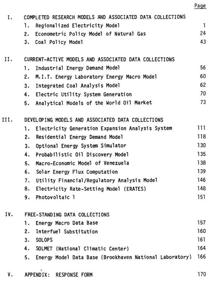
The Regionalized Electricity model (REM) is organized into three major components or submodels, including the demand, supply, and financial regulatory submodels. Figure 1 (see page 19) provides a
the total cost of this financing, the financial/regulatory submodel passes back an estimate of the capital charge rate to the supply submodel. This is used in the generation expansion model as one of the factors determining the amount and type of capital investments in future time periods.
Finally, the financial/regulatory submodel determines the price of electricity and passes this on to the demand submodel. It is assumed that the regulatory process uses data from the current period to set the price for the coming period. Reflecting this, the price information that is given to the demand submodel is used to start the REM simulation for the next time period.
In addition to the information flows among submodels, there are a number of important exogenous inputs to REM. Some of the key exogenous factors are outlined in the ovals of Figure 1.
Thus, the REM model is composed of a mathematically expressed set of behavioral, accounting, and optimization rules. REM is descriptive, not normative, and thus not cast in the mathematically programming mold of many widely known energy modeling efforts. REM contains optimization concepts in parts of its structural detail, but overall it is formulated as a simulation tool with both engineering and economic detail.
In developing the REM model the primary goal was to develop an analytical tool that could be utilized to examine the effects of major national energy policy proposals on electricity prices, electricity demand, and fuel utilization by the electric utility industry.
Thus, the REM fully develops important methodological and analytical issues surrounding the structure and use of the model, as well as shedding some light on a number of important energy policy issues.
b. Data Base
The data collection that supports the REM submodels consists of several sections: U.S. energy demand and fuel prices for the residential commercial and industrial sectors, by state; transmission and
distribution equipment and costs for electric power plants by type of generator and by region; generator characteristics and fuel prices; and regulatory financial parameters. The submodels then contribute a set of input parameters to develop a base case for the simulation.
Scope of the Data Collection
The model treats the U.S. as nine geographic regions: New England, Middle Atlantic, East North Central, West North Central, South Atlantic, East South Central, West South Central, Mountain, Pacific. Some of the data are developed by state for the period 1960-1974 to support the estimation of equations for the demand submodel. Some variables are point estimates, or forecasted values, by region, for the simulation.
schematic overview of the structural components of REM, the linkages among submodels, and the major exogenous variables required to operate the model.
The function of the demand submodel is to estimate the amount of electricity demand in the current time period. Demand for electricity and competing fuels are broken into two major user categories, residential/commercial and industrial, since each consuming sector has different behavioral characteristics, and because the demand for electricity by each sector imposes different requirements on the supply system, particularly regarding transmission and distribution facilities. Demand for electricity and directly competing fuels are estimated for each consuming sector by state. The functional forms for equations and parameter values used are presented in Tables 1 and 2, respectively (see pages 21-22).
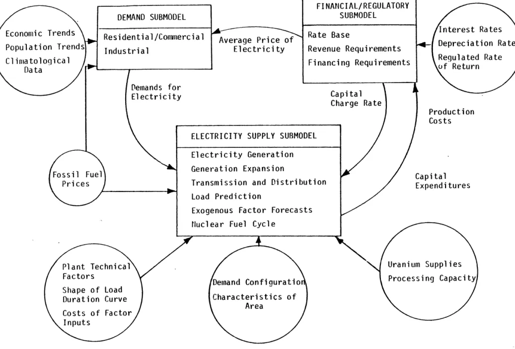
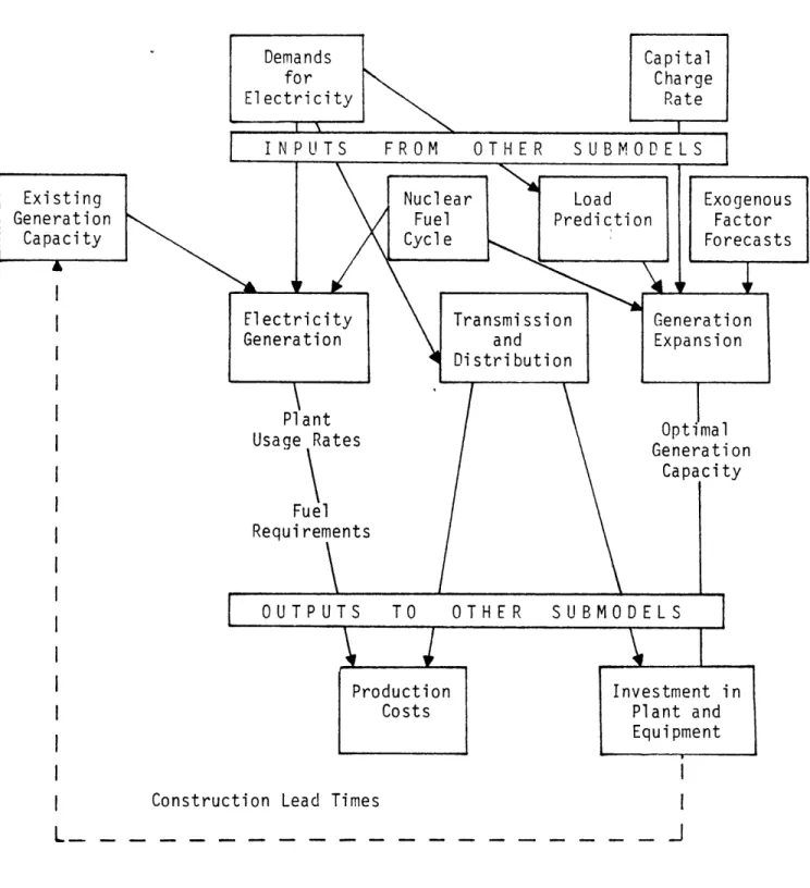
The major behavioral processes in the supply submodel are simulated in three components: electricity generation, generation expansion, and transmission and distribution. In addition, the supply submodel contains three modules that process the input data required by the generation expansion model. These modules deal with load prediction, exogenous factor forecasts, and the nuclear fuel cycle. A schematic outline of the relationship among these components is given in Figure 2.
The financial-regulatory submodel serves two functions. First it applies the tax, accounting, and regulatory rules of the industry to
investment and operating costs of the supply system to determine the price of electricity, and thus closes the supply and demand portions of the model. Second, it simulates the financing of future expansion within the normal guidelines of prudent financial management while maintaining consistency with the income and cash flow accounts and the exogenously supplied costs of alternative forms of capital. By including a regulatory component, REM explicitly recognises that the price of electricity is not set in competetive markets; rather, it is determined by state and federal regulatory authorities using fairly well-established administrative procedures.
The four principal linkages among the REM submodels are indicated by the curved arrows in Figure 1. The demand submodel provides the supply submodel with estimates of the residential/commercial and industrial demands for electricity, the sum of which is the total electricity that must be produced during the current period. Current electricity demand is also an input to the load-prediction component of the supply submodel, where it is combined with previous demands to forecast future demands for
electricity.
The supply submodel provides the financial/regulatory submodel with two primary inputs: production costs and current capital expenditures. These cost estimates are used in the financial/regulatory submodel to determine the revenue requirements of electric utilities and the rate base on which the regulated rate of return is to be calculated. The estimates of capital expenditures are also used to determine the total amount of financing required in the current period. After calculating
The data were converted from kWh into Btus. The range of years available is 1960-1974. Maryland and D.C. sales are combined in the publication, and this figure was split by assigning half to each district. The source used for the residential/commercial sectors' consumption of oil was the Bureau of Mines Mineral Industry Survey's table on "Shipments of Fuel Oil and Kerosine." The data are reported by grade of fuel oil; grades 1-4 were considered assignable to the residential sector and grades 5 and 6 assignable to the commercial sector. The data, reported in barrels, were converted to Btus according to the appropriate fuel grade conversion factor.
Other Variables
A data file was constructed for the average temperature of the three coldest months and the three warmest months, by state. An annual average of the normal monthly average was also calculated. The source of this data is National Oceanic and Atmospheric Administration
publications, for the period 1941-1970.
A consumer price index for all items was constructed. The "Anderson" index for 1970, by state, was used to convert the Bureau of Labor Statistics nationwide CPI. The Anderson index is based on the relative living cost within the SMSAs, available from the Bureau of Labor Statistics, then adjusts this to account for non-metropolitan areas. This deflator assumes uniform inflation rates over all states.
Industrial Sector
In the industrial sector portion of the demand submodel, value-added in manufacturing, price of capital services, and an average energy price were required to estimate total national energy demand. A state's share of the national total is a function of relative state energy costs and population. State fuel demand is divided into the four fuels--coal, gas, oil, and electricity--as a function of relative prices. The data collection that supports this estimation is described below. The cross-sectional time series now stored usually cover the years 1962-1974.
Fuel Prices
The industrial price of natural gas was calculated from data in the Bureau of Mines Minerals Yearbook. The "value and consumption" table does not break out electric utilities through 1967; therefore (total -(residential and commercial)) was used to derive the prices. The descriptive comments for all the data files indicate that the data were converted from MCF to $/Btu by using conversion factors for electric utilities from EEI. The industrial price of oil was constructed using the 1962 average value of the industrial (residual and distillate) oil
price from the Census of Manufacturers, by state. This price was then extended through 1972, using the yearly percentage increases in number 2 fuel oil from the AGA's House-Heating Survey, by state gas utility (see the residential/commercial sector). Data for 1969 were not available and were constructed by interpolation. The units are dollars/Btu. The price of electricity was derived from the EEI's Statistical Yearbook
5
Public sources were used when adequate, and public utility representatives were interviewed when published information was not available.
Demand Submodel Data Collection
The demand submodel focuses on two sectors: the residential/
commercial and the industrial. For both sectors, energy demand and prices were required, in addition to some economic indicators and temperature data. The actual estimates were derived from the 1968-1972 period.
Residential Commercial Sector
For the residential/commercial sector of the demand submodel, consumption per capita was required as a function of a weighted energy price. Fuel-split equations were also estimated, as functions of the relevant fuel prices and temperature.
Fuel Prices
The price of natural gas by state was obtained from the U.S. Bureau of Mines' Mineral Yearbook for the years 1962-1974. The price is derived from value/quantity as reported for the residential and commercial sectors. Where the data are aggregated for some states, the values are equally split and apportioned to the states. A weighted average price is then obtained with each sector's consumption used as weights. The price of electricity was derived from revenues and sales data, available in EEI's Statistical Yearbook for the years 1962-1974. Although there is a specific category for "residential," there is none for the commercial sector. Therefore, the category "small light and power" was assumed to be a comparable definition of the commercial sector. A weighted average price was calculated, using each sector's usage share of the fuel as weights. The final data files are in units of current dollars/Btu. An average oil price appropriate for the residential/commercial sector was not available to the researchers. The American Gas Association's price for number 2 fuel oil, by state, for the years 1962-1974, was used. The data are reported in the source in cents/gallon, and were converted to current dollars/million Btus.
Fuel Consumption
Data for the consumption of natural gas by residential and commercial sectors were obtained from the annual quantities by state tables in the Bureau of Mines Minerals Yearbook. The units were converted from million cubic feet to Btus using state-specific conversion factors in the EEI Statistical Yearbook of the Electric Utility Industry. Where the reported data were not completely disaggregated by state, the total was split and equally apportioned to the states. Annual sales data by state from the EEI Statistical Yearbook were used to derive electricity consumption. As described in the price data section, the commercial sector is not explicitly defined and the "small power and light" category was assumed to be comparable.
tables on revenue and sales, by state, for large light and power. This category includes some of the commercial sector and excludes some small industrial. Where states are aggregated, the quantity was equally split and apportioned to the states. The data were converted to dollars/Btu from kWh. The 1962 value for the industrial price of coal was obtained from the Census of Manufacturers. This was then extended to 1972 using the increases in the price of coal to electric utilities from the EEl's Statistical Yearbook. Where prices for states were unavailable, gaps in the data series were filled by adding transportation costs to the fuel prices of neighboring states. These transportation costs are all listed in the stored data files.
An average weighted price, by state, was calculated using consumption of each fuel as weights. This average state fuel price was then used to calculate a weighted average U.S. price, using each state's total industrial fuel consumption as weights.
Other Variables
Total resident population (including military) was obtained for all states for the period 1960-1974 from the Bureau of the Census. Data are
published in thousands, and were converted to singular units. Land area for each state from the U.S. Statistical Abstract was also collected and stored and a data series for population/square mile/state was created.
Value-added, by state, for the years 1962-1972, was obtained from the Census of Manufacturers and the Annual Survey of Manufacturers. Data for the SIC codes 20-39 for all states are stored in separate data files for each year. These are then combined to form a file of the total for each state, years 1962-1972. There is also a file for total national value-added, years 1947-1971, but no source is indicated.
A price index with base year 1967 was used to deflate currency data. The data series range for the WPI is 1947 to 1974. There are
separate series for an industrial price index, an industrial coal price index, and a refined oil products price index, but the source of these last three indices or the application to deflate specific prices series
is not indicated.
Supply Submodel
Within the supply submodel, the nine regions each have five plant types plus the exogenously specified hydro available as supply alternatives. Each plant is characterized by a set of economic and technical data as a function of time; specifically, a capital cost, a fuel cost, an operation and maintenance cost, and a conversion efficiency. Each plant type is further assigned a forced outage rate, a duty cycle, and a lead time.
The relationship of transmission and distribution equipment to demand and the operation and maintenance cost have been estimated from historical data, while a structured analytical treatment was used for
generation planning and electricity production. The data that supports the empirical work will be described in a separate section, because it is cross-sectional, time-series data, obtained for the most part from published sources. This portion of the supply submodel also interfaces with the demand submodel. The variables for generation and expansion are the results of simple expectation formation relationships based on point estimates.
Data Developed for the Purpose of Estimation
Operation and Maintenance Costs: Transmission and Distribution
The data collection ranges from 1967-1973, from three-year published averages. The components of cost are interactive in nature, and it is difficult to obtain accurate cost data; therefore, aggregate expenditures and equipment additions were used as average costs. Costs of transmission lines were obtained for the previously defined nine U.S. regions. This cost was defined as the ratio of the sum of undefined capital expenditures to the sum of new structure miles (or cable miles for underground) energized. Overhead and underground are divided into two categories: high volt and low volt. The source of these data is the "Annual Statistical Report" of Electrical World. The cost of primary distribution lines is derived in the same manner as cost of transmission lines and from the same source. The researchers report that the size of the sample for distribution lines is much larger than that for transmission lines; therefore, there is less variability and this series is more reliable. Three-year aggregate averages for transmission substation costs for the period 1953-1973 were obtained from the "Annual Statistical Report" of Electrical World. The units are dollars/kilowatt ampere of installed capa-city.
Other Costs: Distribution Substations, Line Transformers, and Meters There is no comprehensive source of data for these items. They are, however, not considered to be a major component of the cost of delivered electricity, and therefore not as important for the estimation. For these variables, point estimates were obtained from New England electric utility company representatives and other private sources.
Transmission and Distribution Equipment
This section of the supply submodel relates demand and other characteristics of a service area to the following six equipment items: transmission lines (in structure miles), transmission substations (in kilowatt amperes capacity), primary distribution lines (in circuit miles), distribution substations (in kilowatt amperes capacity), line transformers (in kilovolt amperes capacity), and meters (in number). These data were obtained for the period 1965-1972 from the Federal Power Commission's Statistics of Privately Owned Utilities. Privately owned
utilities' data were deemed sufficient since they account for 80% of the entire electric utility industry and the data are more consistently reported. The equations derived from this estimation are preserved in
Generation Planning and Electricity Production Fuel Costs
Fossil Fuel Prices
For the input base case, fossil fuel price start values are required. These data points, obtained for 1975 for fossil fuels, are an approximation of an historical price, derived in the following manner: A price at the minemouth or wellhead, as a national average, is the base, to which a transportation cost for each of the nine regions is added to
derive a regional price. The source used for the price at the wellhead or minemouth is not cited, and the derivation of the transportation costs also is not described. However, all of the values used are presented in tables in Appendix D of Electric Power in the U.S. Escalation rates are used for the future years.
Although the source and derivation of the prices were not available at this writing, we are told that coal prices should be considered a composite price because the cost of coal scrubbers was incorporated where appropriate (for certain regions). The oil price for 1975 is an average of the three-tier domestic oil price and the imported price. Costs of transporting and refining are added to obtain regional prices.
Light Water Reactor Fuel Cycle
Nuclear fuel cycle costs that are used to determine nuclear fuel direct costs and carrying charges are exogenous to the model. The basic data from which the flow rates and total fuel cycle costs were calculated were obtained from ERDA. The 1975 unit costs obtained for Uranium Oxide feed, conversion enrichment/fabrication, shipping fresh and spent fuel, waste disposal, reprocessing, U credit and Pu credit, and carrying
charges are presented in Appendix D of Electric Power in the U.S. Capital Costs
A survey of a large number of utility companies throughout the U.S. and a review of estimates within the literature were undertaken to obtain capital costs for New England plants. The components of capital cost are the cost of the base plant, cost of the cooling plant system, cost of air pollution equipment, and interest during construction. Multipliers were used to convert the New England values to capital costs for each of the nine regions. These were obtained from the Atomic Energy Commission's publication, Power Plant Capital Costs, Current Trends and Sensitivity to Economic Parameters. Load factors by region were obtained from the Edison Electric Institute, the 55th Annual Election Power Survey, 1974.
Financial-Regulatory Submodel
The parameters used for the financial-regulatory submodel were the regulated return on equity, the cost of debt, the cost of preferred stock, the debt limit, the minimum interest coverage ratio, the preferred stock fraction, and the cost of SBB financing.
The regulated rate of return on equity is based on the rate base plus allowance for working capital. The valuation of the rate base chosen for this model was cost less accumulated depreciation, based on a 40-year lifetime. The allowance for working capital was calculated using the FPC formula for monthly billing companies. The source for the valuation of the rate base is not cited.
Operation and maintenance cost and fuel cost are from the output of the supply submodel. Taxes, depreciation, deferred taxes, allowances for interest during construction, investment tax credits, and preferred and common stock dividends are computed within the financial submodel.
c. Computer Aspects
The model is in the form of a source program (written in FORTRAN) and a number of data sets. The source program consists of the MAIN program along with certain subroutines and functions. The data sets are stored in the FORTRAN files, which are referred to within the source program by their numbers.
A simulation involves creating a load module from the source program and executing it using the data inputs in the FORTRAN file.
A detailed documentation of the REM model that describes the different capabilities of the model and enables users to use the model for various policy analysis purposes is available in mimeo form under the title "Documentation of the Regionalized Electricity Model" by Dilip P. Kamat, University of Texas at Austin, June 1976.
The original model was designed to be run in FORTRAN on an IBM 360. All the results documented in the original articles were obtained through this system. All recent work on the demand submodel has been done through TROLL, operating on the IBM VM/370, referred to as CMS
(Conversational Monitor System).
Most of the data developed for the model are stored on magnetic tape. The demand data collection is stored in TROLL format, through the TROLL computer system of the Massachusetts Institute of Technology in both one-and two-dimensional data files.
The supply data collection and the financial submodel input parameters are stored on magnetic tape in FORTRAN compatible format. No technical tape descriptor is available, but the tapes can be read with CMS tape default values.
The transmission and distribution equipment data is not available at the M.I.T. Energy Laboratory, but a copy of the data is being used by researchers at the University of Austin, Texas.
A detailed description of the different data sources and a description of the input data for base case simulation are described in the Appendices of Electric Power in the U.S. by Martin Baughman, Paul Joskow, and Dilip Kamat.
1.3 APPLICATIONS AND PLANNED FUTURE DEVELOPMENT
REM is now being. utilized by a number of researchers around the country.
Martin Zimmerman at MIT is incorporating specific regional coal supply functions into the model. Dale Jorgenson at Harvard is integrating the model with an aggregate model of the economy that will eventually capture inportant interrelationships between the electricity sector and the economy as a whole.
The ERDA Light Water Reactor (LWR) Program Strategy Analysis and Evaluation Project conducted by the Energy Laboratory at MIT has also applied the REM model framework to evaluate the technical advances in the construction and operation of LWRs in terms of their potential for decreasing construction and operating costs associated with delivering electricity.
The MIT model assessment group has compiled a list of potential policy applications, as shown in Table 3 (see page 30).
Martin Baughman and Dilip Kamat at the University of Texas are currently working with a modified version of the REM model.
Keith David Brown at The University of Texas, Austin, has come up with a monthly production simulator for the REM that presents a method of simulating the process of bulk power production that improves on the method used in the REM developed by M.L. Baughman and P.L. Joskow.
1.4 LIST OF WORKING PAPERS, ARTICLES, AND BOOKS (generated by the REM Project): Baughman, M.L. and Joskow, P.L., "A Regionalized Electricity Model," MIT
Energy Laboratory Report No. MIT-EL 75-005, Cambridge, MA., Dec. 1974. This document reports on research in progress. In Chapter 1, the authors review the economic principles of electric utility behavior, both in the operations and planning spheres. In Chapter 2, the authors discuss how these principles have been combined into the specification and development of an engineering-econometric simulation model for electric utility behavior. Finally, in Chapter 3, the results of some sample simulations done with the substitution possibilities inherent in the model structure exemplify how it can be used. Since this is a report on work in progress, the simulations discussed are not to be reviewed as forecasts but rather as examples of model use.
Baughman, M.L. "Documentation and User's Manual for Interfuel Competition Model V.3 FORTRAN," Sept. 1973, mimeo.
The Interfuel Competition Model (V.3) is basically an engineering/economic simulation program for the medium to long-range
(3-30 year) interactions of the major primary fuels and secondary energy sources (coal, oil, natural gas, nuclear fuels, and electricity) in the U.S. energy consuming markets. The purpose of the model is to match the consuming sector demands with the energy supplies in a way that is consistent with consumer preferences and relative fuel prices. The purpose of this document is to acquaint potential users and interested parties with some of the capabilities of this model.
Baughman, M.L. and Joskow, P.L., in association with F.S. Zerhoot, "Interfuel Substitution in the Consumption of Energy in the United States," MIT Energy Laboratory Report No. MIT-EL 76-002, Cambridge, MA., May 1974.
The effects of alternative public policies on the consumption and prices of various forms of energy in the United States depends critically on the nature of consumer demands for fuels and the supply characteristics of these fuels. Previous work on energy demand has tended to concentrate on the demand for particular fuel as determined by
standard economic variables such as the price of the fuel, income levels, sometimes the price of alternative fuels, and other demographic characteristics of the consuming population. In this work the consumer decision-making process is viewed as being composed of two steps. First, the consumer decides that he wants a particular service and, second,
seeks to find the fuel that will provide this service most cheaply. This view leads the authors to concentrate on substitution possibilities among
fuels for particular. services rather than own-pric3 elasticities for a particular fuel.
This paper presents results for the determinants of energy consumption in the residential and commercial sector in the United States. First, a discussion of the conceptual model used for fuel choice decisions is presented. Then, empirical results are given for appliance choices in the residential sector for four selected appliances and for the "fuel-split" of aggregate energy consumption among the three fuels used in the residential and commercial sector. The own-price and cross-price elasticities are estimated and discussed.
Next, the paper discusses the determinants of total energy demand in the residential and commercial sector and presents empirical results for a simple flow adjustment model. The long-run price elasticity of total demand in this sector is estimated to be about -0.5, while the short-run
(one-year) value is -0.15. Finally, the estimated relationships are used to make projections to 1980 for alternative price scenarios. These results show that significant consumption responses to changing fuel prices can be expected and, further, that some states are much more dramatically impacted than others.
Baughman, M.L. and Joskow, P.L., "Energy Consumption and Fuel Choice by Residential and Commercial Consumers in the United States," Energy
Systems and Policy, Crane, Russak and Company, Inc., 1975.
The purpose of this paper is to report the conceptual design and estimation results of models for total demand and aggregate fuel choice decisions in the residential and commercial sectors. The authors started with the view that fuel utilization decisions can be separated into a two-level decision process. First, the consumer decides on the level of energy-using services he/she desires to meet his/her functional needs,
then seeks to find the combination of fuels that will provide these services most cheaply. This dichotomy formed the basis for the models actually adopted.
The model used to explain total demand for energy in the residential and commercial sectors is a simple flow adjustment model. The long-run price and income elasticities of demand in this sector were estimated to be about -0.50 (after adjustments of fuel mix) and 0.6, respectively. The short-run (one-year) elasticities were about 16% of these values.
A set of simulations were performed using alternative scenarios about the evolution of future prices. The results show that much conservation can be expected to take place in the residential and commercial sectors as a result of past and expected future price increases. When comparing the model behavior with that used by the FEA in its Project Independence analyses, the differences indicated that the FEA overestimated future energy consumption trends for the residential and commercial sector. Also, in response to President Ford's proposed taxes on oil, the model exhibits little additional shift away from that fuel above that expected purely in response to the existing increase of oil prices to $11 per barrel.
Baughman, M.L. and Joskow, P.L., "The Effects of Fuel Prices on Residential Appliance Choice in the United States," Land Economics, February 1975.
In this paper the authors seek to estimate the effects of fuel prices on the fuel choice decisions by residential consumers for four important energy usage categories for which consumers face two or more fuel alternatives: space heating, water heating, cooking, and clothes drying. These usage categories account for approximately 80% of residential energy consumption in the United States. Explicit specifications and empirical results for the application of the logit model of fuel choice to the appliance decisions of residential consumers for four types of appliances are presented in this paper.
Kamat, D.P., "A Financial/Cost of Service Model for the Privately Owned Electric Utility Industry in the United States," Master of Science Thesis, Alfred P. Sloan School of Management, Massachusetts Institute of Technology, Cambridge, MA., June 1975.
In the recent past, electric utilities have faced serious financial problems. Operating and capital costs have been rising due to increased fuel costs, interest rates, and tightened environmental constraints. This has resulted in reduced profits for the utilities; hence, they are attracting less capital. Many solutions have been suggested to solve this problem of capital shortage, all of which have varied impacts on the future of electric utilities. The purpose of this thesis was to build a financial model that could analyze the effects of these policy changes suggested to relieve the capital shortage. This model was then hooked up with a regionalized electricity model at the Energy Laboratory, MIT, and it was possible to get elaborate scenario simulations of the electric utility industry for the various policy alternatives. The study concludes that many of the suggested changes, such as increased
investment tax credits, are not as effective as publicized, whereas others, such as inclusion of construction work in progress in the rate
base, have a major impact.
Joskow, P.L. and MacAvoy, P.W., "Regulation and the Financial Condition of the Electric Power Companies in the 1970s," American Economic Review, 65, May 1975.
The purpose of this paper is to assess the financial prospects of the nation's electric utility industry, given existing regulatory institutions and continued high rates of growth of demand in the late 1970s.
Bottaro, D.J. and Baughman, M.L., "Estimation of Transmission and Distribution Equipment Needs," MIT Energy Laboratory Working Paper, MIT-EL 75-001WP, Jan. 1975.
This paper is the first in a series estimating the capital equipment needs, capital costs, and operation and maintenance expenses of the transmission and distribution systems in the electric power sector.
Sequeira, S.G. and Baughman, M.L., "Engineering Estimates of Transmission and Distribution Equipment Costs," MIT Energy Laboratory Working Paper MIT-EL 75-002WP, Cambridge, MA., March 1975.
This paper is the second in a series estimating the capital equipment needs, capital costs, and operation and maintenance expenses of
the transmission and distribution systems in the electric power sector. The paper reviews data on the costs of distribution transformers (for
both overhead and underground systems), distribution substations, transmission and distribution lines, transmission substations, and the cost of metering systems, both for residential and large commercial and industrial consumers.
Baughman, M.L. and Bottaro, D.J., "Electric Power Transmission and Distribution Systems: Costs and Their Allocation," IEEE Transactions on Power Apparatus and Systems, P.A.S.-95, May/June 1976.
The costs derived from installing, operating, and maintaining the transmission and distribution system have historically comprised about 2/3 the total costs of producing and delivering electricity to residential/commercial customers, and over 1/3 the total costs of
supplying electricity to large industrial customers. This paper estimates the cost of transmission and distribution for nine regions of the United States for the above two customer classes. These costs are
detailed for six categories of equipment used in the transmission and distribution system and the contribution to the total cost of each equipment category is determined.
Joskow, P.L., "The Future of the U.S. Nuclear Energy Industry," Bell Journal of Economics and Management Science, Spring 1976.
This paper examines the demands for nuclear reactors, raw uranium, and fuel-cycle requirements by the U.S. electric utility industry over the next 20 years, under a number of different possible states of the world. The analysis is performed by using the MIT Regional Electricity Model (REM) developed by the authors. This model is an engineering-econometric-financial simulation model of the electric utility industry in the United States. It includes a supply submodel, a demand submodel, and a regulatory financial submodel. The analysis indicates that demands for reactors, raw uranium, and uranium enrichment, will be substantially below the projections made by such government
agencies as the Atomic Energy Commission. These demands are shown to be very sensitive to the costs of air pollution control affecting coal
utilization, the costs of uranium and uranium enrichment, the price of oil, and electric utility regulatory practices. It appears that in almost all cases existing-plus-planned expansion of government-owned enrichment facilities will be sufficient to meet domestic needs until the mid-1980s. However, the continued financial viability of the five reactor vendors serving the domestic market is doubtful. Two or three of these vendors will either have to drop out of the market or obtain increased nuclear steam supply system orders from foreign countries.
Joskow, P.L. and Rozanski, G., "Utilization by the Electric Utility Industry in the United States, 1975-1995," MIT Energy Laboratory Working Paper No. MIT-EL 76-006WP, May 1976.
In this paper the authors make use of the MIT Regionalized Electricity Model (REM) to examine the course of future electricity consumption and fuel utilization by the electric utility industry for the U.S. as a whole as well as for each of the nine census regions in the U.S.
Baughman, M.L., Joskow, P.L., and Kamat, D., Electric Power in the United States: Models and Policy Analysis, MIT Press, Cambridge, MA., 1979.
This book reports the results of several years of research aimed at the development and application of an engineering-economic model of the electric power industry in the United States. This model is known as the Regionalized Electricity Model (REM).
In this book the authors have attempted to do two things. First, they have presented a. detailed discussion of the structure and behavior of the Regional Electricity Model (REM), a computer simulation model
developed over the past few years to facilitate understanding the effects of a variety of public policies on the electric utility industry in the United States. Second, the model has been used to examine the likely effects of public policies that appear to have some prospect of being
implemented in the next few years.
The REM Model reflects the authors' perceptions of the need for a computer-based simulation model of the electric power sector in the United States, to be used as an aid in formulating and evaluating alternative public policies as they affect the supply and demand for electricity.
Kamat, D.P., "A Documentation of the Regional Electricity Model," mimeo. The purpose of this document is to acquaint potential users and other interested parties with the multifaceted capabilities of this model and enable them to use it for various policy analyses.
Joskow, P. and Mishkin, F., "Electric Utility Fuel Choice Behavior in the United States," International Economic Review, October 1977.
This paper attempts to depart from the traditional (differentiable aggregate production function) specification of electricity production, using instead conditional logit analysis. The fuel choice of an electric utility for a new fossil-fuel based, load steam-electric plant is analyzed to explicitly account for the discreteness of fuel-burning techniques available to the firm. For this purpose a probability model
of the conditional logit form is specified and estimated using maximum likelihood techniques.
MIT Model Assessment Group. "Independent Assessment of Energy Policy Models: Two Case Studies," EPRI EA-1071, Final Report, MIT Energy Laboratory, Cambridge, MA., May 1979.
Energy policy models are playing an increasingly important and visible role in supporting both private and public energy policy research and decision making. As their importance has increased so too has the need for model review and assessment to assist in establishing model credibility for users and those affected by model-based policy research. Toward this end EPRI had sponsored the MIT Energy Laboratory in a one-year project to assess two important energy system models, the Baughman-Joskow Regionalized Electricity Model and the Wharton Annual Energy Model , and to identify and analyze organizational and procedural issues in the model assessment process.
Mostafa, M., "Regional Analysis of Transmission and Distribution Needs and Costs in the United States," Master of Science Thesis, Center for Energy Studies, The University of Texas at Austin.
Regression analysis is used to estimate equations for six major equipment items and the three types of operation and maintenance expenses
for transmission and distribution of electricity. The United States is divided into nine census regions, and equations are estimated for a pooled national aggregate and each census region. A ten-year time. series
of cross-sectional data for privately owned utilities are used to perform the regressions using ordinary least-squares technique.
Also, a survey of the capital costs of the six equipment items, which contribute significantly to the total cost of transmission and distribution system, is presented.
Finally, the contribution of the cost of each transmission and distribution equipment item and the operation and maintenance expenses of these systems to the total cost of electricity for residential, small light and power, and large light and power customers are computed.
White, D.E., "Extensions and Revisions of the MIT Regional Electricity Model," MIT Energy Laboratory Working Paper MIT-EL 78-018WP, Cambridge, MA., July 1978.
This paper reviews some of the changes made in the MIT Regional Electricity Model (REM) from September 1976 to May 1978. These changes were made either to better evaluate some energy policy questions or to better represent energy sector behavior.
Brown, K.D., "Implementing a Monthly Production Regional Electricity Model," Working Paper, Center The University of Texas at Austin, June 1979.
This paper electric power This production Baughman-Joskow method previousl Simulator for Energy
presents a method of simulating the process of production on a regional basis for the United Sta
simulation method is designed for implementation in Regionalized Electricity Model (REM) and improves on y used in REM.
Improvements in the new production simulation model in comparision with the previous one include:
a. incorporation of 17 types of generation plants instead of 9; b. simulation of production on a monthly basis, rather than
annually;
c. scheduling plant capacity monthly basis, rather than are met during annual offpeak
for maintenance on assuming maintenance
periods; and
a levelized requirements d. modeling pumped storage generation for peak sharing, and
pump-lack load for monthly off-peak demand.
for the Studies, bulk tes. the the
4 4 Economic Trends Population Trends Climatological Data DEMAND SUBMODEL Residential/Commnercial Industrial Demands fo Electricit Fossil Fuel Prices Average Price of Electricity r y Capital Charge Rate
j
FINANCIAL/REGULATORY SUBMODEL Rate Base Revenue Requirements Financing RequirementsUranium Supplies
Processing Capacity Plant Technical Factors Shape of Load Duration Curve Costs of Factor Inputs Demand Configuratio Characteristics of AreaFIGURE 1. SCHEMATIC OVERVIEW OF THE STRUCTURE OF THE BAUGHMAN-JOSKOW MODEL
Interest Rates Depreciation Rates Regulated Rate of Return Production Costs Capital Expenditures ELECTRICITY SUPPLY SUBMODEL
Electricity Generation Generation Expansion
Transmission and Distribution Load Prediction
Exogenous Factor Forecasts Nuclear Fuel Cycle
Electricity Transmission Gen(
Generation and Ex p
Distribution
Plant Opt
Usage Rates GenE
CaF Fuel
Requirements
I
OUTPUTS Production TO OTHER SUBMODELSInvestmE
Costs Plant
Equipn
I Construction Lead Times
L
FIGURE 2. SCHEMATIC OUTLINE OF THE COMPONENTS OF THE REM SUPPLY SUBMODEL al tion ity
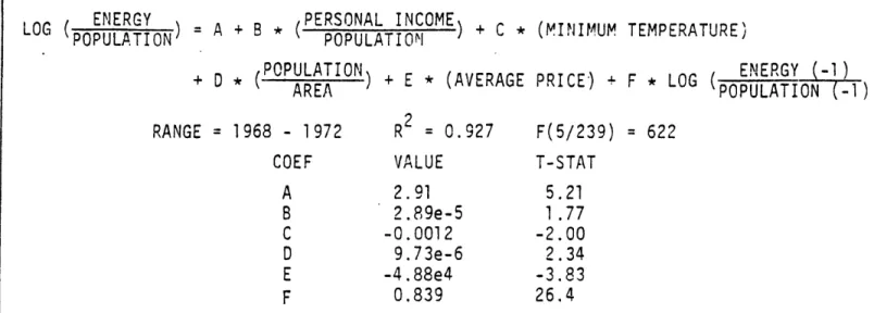
LOG ( NERGY = A + B (POPULATIO ) + C * (MINIMUM TEMPERATURE)
POPULATION POPULATION
+ D * POPULATION ENERGY (-1)
AREAD ( E * (AVERAGE PRICE) + F * LOG (POPULATION -)
AREA POPULATION (-1) RANGE = 1968 - 1972 COEF A B C D E F R2 = 0.927 VALUE 2.91 2.89e-5 -0.0012 9.73e-6 -4.88e4 0.839 F(5/239) = 622 T-STAT 5.21 1.77 -2.00 2.34 -3.83 26.4
GAS GAS PRICE
LOG GAS ) = A + C * LOG (ELECTRICITY PRICE
ELECTRICITY ELECTRICITY PICE
+ D * (MAXIMUM TEMPERATURE)
GAS
+ F * (MINIMUM TEMPERATURE) + H * LOG (ELECTRICITY (-1)
OIL OIL PRICE
LOG (ELECTRICITY + C * LO (ELECTRICITY PRICE + E * (MAXIMUM TEMPERATURE)
+ G * (MINIMUM TEMPERATURE) + H * LOG (ELECTRICITY (-1)OIL (-1) RANGE = 1968 - 1972 COEF A B C D F G R2 = 0.954 VALUE 0.07 0.208 -0.137 -0.0015 -0.0022 -0.0022 -0.0063 0.897 F(7/482) = 1462 T-STAT 0.56 1.65 -3.29 -1 .O -1.58 -1.74 -3.19 66.0
TABLE 1. RESIDENTIAL AND COMMERCIAL DEMAND PELATIONSHIPS I a
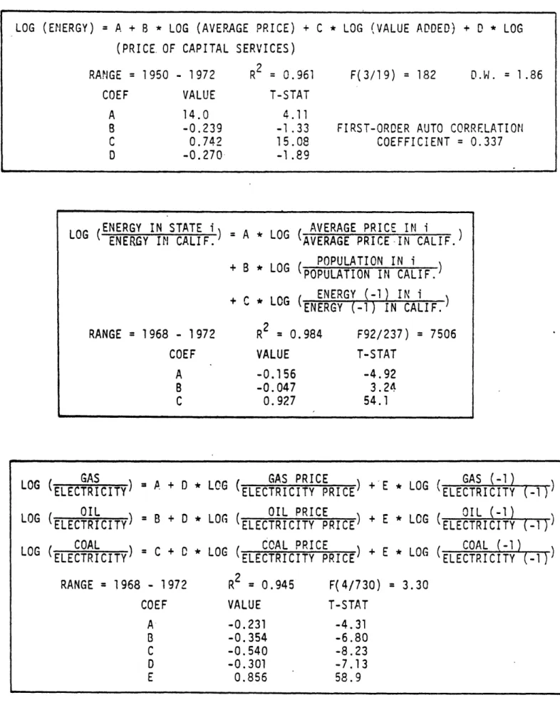
LOG (ENERGY) = A + B * LOG (AVERAGE PRICE) + C * LOG (VALUE ADDED) + D * LOG (PRICE. OF CAPITAL SERVICES)
RANGE = 1950 - 1972 COEF VALUE 14.0 -0.239 0.742 -0.270 R2 = 0.961 T-STAT 4.11 -1.33 15.08 -1 .89 F(3/19) = 182 D.W. = 1.86
FIRST-ORDER AUTO CORRELATION COEFFICIENT = 0.337
ENERGY IN STATE i ENERGY IN CALIF.)
AVERAGE PRICE IN i
- A . LOG (AVERAGE PRICE IN CALIF.)
POPULATION IN i POPULATION IN CALIF. ENERGY (-1) IN i +C OG (ENERGY (-1) IN CALIF. RANGE = 1968 - 1972 COEF A B C R2 = 0.984 VALUE -0.156 -0.047 0.927 F92/237) = 7506 T-STAT -4.92 3.24 54.1 GAS LOG ( LOG ELECTRICITY)GAS
OIL
LOG ( ELECTRICITY)OI COAL ELECTRICITY
GAS PRICE LOG
A + D LPG (ELECTRICITY PRICE
A + D * LOG ( ) + E * LOG
ELECTRICITY PRICE
= C + LOG PRICE ) + E * LOG ELECTRICITY PRICE RANGE = 1968 - 1972 COEF A B C D E R2 = 0.945 VALUE -0.231 -0.354 -0.540 -0.301 0.856 GAS (-1) ELECTRICITY -1 OIL (-1) (ELECTRICITY (-1) COAL (-1) ELECTRICITY (-1) F(4/730) = 3.30 T-STAT -4.31 -6.80 -8.23 -7.13 58.9
TABLE 2. INDUSTRIAL DEMAND RELATIONSHIPS
-Table 3: Potential Policy Applications 1. Changes in factors affecting electricity demand growth paths
- economic/demographic trends - conservation policies 2. Load management - peak-load pricing* - cogeneration - seasonal pricing
3. Impacts of changes in cost factors - capital costs for new plants - fuel prices*
- wage rates
- taxes (possibly a Btu tax)
4. Changes in resource supply conditions - resource constraints*
- increasing cost supply schedules 5. Costs of financing*
6. Industry responses to capital "shortage" - state financing*
- less capital-intensive technologies - reduce growth
- reduction in plant reserve margin 7. Regulatory policies
- regulated rate of return*
- inclusion of work in progress in rate base* - exclusion of noneconomic plants from rate base* - regulatory lag
8. Alternative lead times for capacity expansion* 9. Environmental constraints
- siting restrictions
- capital equipment requirements* - increased operating costs* 10. Technology assessment
- advanced generation technologies: centralized and distributed conventional and nonconventional cogeneration fuel conversion - nuclear: non-LWR, breeder, etc.
- storage - T and D
2.1 MODEL HISTORY
a. Name: An Econometric Policy Model of Natural Gas
b. Developers: Paul W. MacAvoy, Department of Economics, Massachusetts Institute of Technology, Cambridge, Massachusetts; currently at Yale University, New Haven, Connecticut
Robert S. Pindyck, Sloan School of Managment, Massachusetts Institute of Technology, Cambridge, Massachusetts
c. Duration: 1972 to 1974 1977 to 1978
d. Location: MIT Energy Laboratory, Cambridge, Massachusetts e. Sponsor: National Science Foundation
1.2 MODEL DESCRIPTION a. Summary
The economic model of natural gas markets with explicit policy controls is built and simulated to predict and analyze the effects of alternative regulatory policies. The model consists of a set of econometric relations among several policy-related variables. It provides a vehicle for performing simulations into the future using different policy options, so as to indicate the effects of the options on the levels of prices and the size of the shortages. Thus, its formulation stresses price, reserve quantities, production quantities, and associated demands for production.
The econometric model has the important characteristics of:
a. simultaneously describing the behavior of both reserves and production markets;
b. describing the regional organization of the industry at a disaggregated level; and
c. accounting for the time-dynamics inherent in the various activities of the industry.
The natural gas industry is viewed as a complete system. Most previous econometric studies of natural gas (e.g., Balestra) have investigated either supply or demand but have neglected the simultaneous interactions of the two. The present model accounts for the simultaneous interaction of output and demand of both field and wholesale levels of the industry.
Regulation has been in effect for both field sales and transportation of gas. Consequently two distinct sets of markets are accounted for in modeling the gas industry. Production and demand are described in both the market for reserve additions and the market for wholesale deliveries. These markets are reiona in nature; reserve additions are contracted for in regional field markets and gas production is delivered by pipelines to regional wholesale markets. These regional markets are interconnected through the network of natural gas pipelines across the country. The spatial organizations of these markets have been accounted for in the model.
The time dynamics of different stages of reserve accumulation, production, and demand are an important aspect of the model. Attempts
have therefore been made to include appropriate time lags in all the relationships in the model.
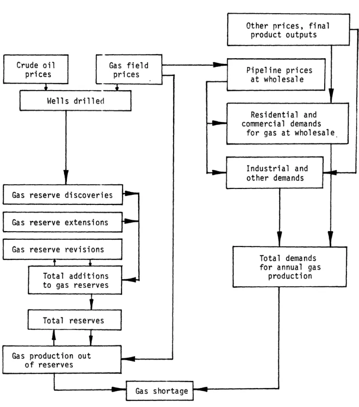
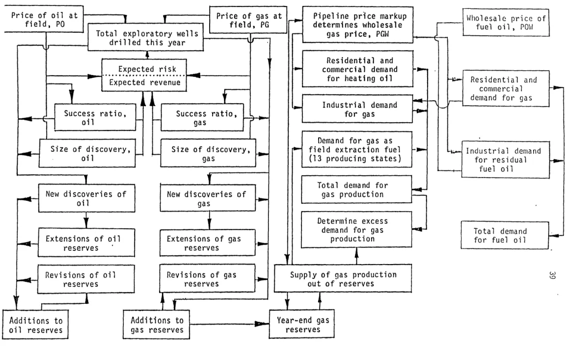
A simplified diagram of the econometric model is shown in Figure 1 (see page 38) and a block diagram of the model is presented in Figure 2 (see page 39). The block diagram provides an overview of both the model's organization and the relationship between field and wholesale markets.
This block diagram provides a good starting point for understanding the model's structure.
The producer, in the gas and oil reserves market, engaged in exploratory activity has, at any point in time, a portfolio of drilling options available on both extensive and intensive margins. In deciding whether or not to drill, producers make a trade-off between expected risk and expected return, and thereby decide whether additional drilling will be extensive or intensive. This choice is influenced by changes
(or expected changes) in economic variables such as field prices of oil and gas and drilling costs. The model developed here has an equation for wells drilled that is based on a rational pattern of producers' responses to economic incentives in forming their portfolios of
intensive and extensive drilling. Drilling alone does not establish discoveries in the model. Equations are specified to determine the fractions of wells drilled that will be successful in finding gas, and the fraction successful in finding oil. The "success" ratios depend on whether economic incentives (e.g., price increases) result in drilling on the extensive or intensive margin (and this must be determined empirically). Two equations determine the size of discovery per
successful well for gas and oil respectively. Discovery size is related to the number of successful wells drilled previously and to the volume of previous discoveries in that region, as well as to gas and oil prices.
Finally, the model generates forecasts of new discoveries from this set of equations. Total new discoveries (calculated for gas and oil) separately are the product of number of wells, success ratio, and size of find per successful well. This level of detail permits explicit consideration of the process of long-term geological depletion as well
Addition to reserves also occurs as a result of extensions and revisions of existing reserves. These extensions and revisions for both gas and oil depend on (1) price incentives; (2) past discoveries of gas and oil; (3) existing reserve levels for both gas and oil; and (4) the cumulative effect of past drilling.
Thus, additions to gas reserves are the sum of new discoveries, extensions, and revisions. Aside from changes in underground storage, subtraction from gas reserves occurs as a result of production. Similarly, additions to oil reserves are the sum of new discoveries of oil, extensions, and revisions. Since the model does not explain the production of oil from reserves, year-end oil reserves are not determined. These partly engineering, partly economic equations determine addition to reserves made by petroleum companies.
The level of natural gas production out of reserves depends not only on the size of the reserve base, but also on prices that buyers are willing to pay. The formulation of production supply in this model has the marginal cost of developing existing reserves determine a particular level of annual flow. Marginal production costs are dependent on reserve levels relative to production, so as the reserve-to-production ratio becomes smaller, marginal costs rise sharply. Thus, as can be seen in the block diagram, the level of gas production out of reserves is a function of both the field price of gas and quantity of year-end reserves in any one production district.
The wholesale demand for natural gas production is a function not of the wellhead price of gas but rather of the wholesale price. Average wholesale prices for gas are computed in the model for each consumption region in the country through a series of pipeline price markup equations. The price markups are based on operating costs, capital costs, and regulated rates of profit for the pipeline companies.
Of course, wholesale gas prices are not the only determinants of wholesale gas demand. Residential and commercial demand, and industrial
demand, depend as well on the prices of alternative fuels (including the wholesale prices of oil) and "market-size" variables such as population,
income, and investment, which help determine the number of potential consumers. Separate residential-commercial and industrial equations are formulated for each of five regions of the country. A third category of natural gas demand formulated within the model is the demand for gas as field extraction fuel.
Natural gas is competitive with fuel oil both in industrial and residential/commercial markets. The model therefore contains a set of wholesale demand equations for fuel oil. The fuel oil demand equations have the same structural form as do the natural gas demand equations, thus making it possible to compare changes in oil and gas demand in a consistent manner. As can be seen from the block diagram, these demands
for oil depend on the wholesale prices for both oil and natural gas, and also on the same "market size" variables as gas demand.