HAL Id: hal-00626172
https://hal.archives-ouvertes.fr/hal-00626172
Submitted on 27 Aug 2020
HAL is a multi-disciplinary open access
archive for the deposit and dissemination of
sci-entific research documents, whether they are
pub-lished or not. The documents may come from
teaching and research institutions in France or
abroad, or from public or private research centers.
L’archive ouverte pluridisciplinaire HAL, est
destinée au dépôt et à la diffusion de documents
scientifiques de niveau recherche, publiés ou non,
émanant des établissements d’enseignement et de
recherche français ou étrangers, des laboratoires
publics ou privés.
Multispectral imaging the sun in the ultraviolet
Thierry Dudok de Wit, Saïd Moussaoui, Pierre-Olivier Amblard, Jean
Aboudarham, Frédéric Auchère, Matthieu Kretzschmar, Jean Lilensten
To cite this version:
Thierry Dudok de Wit, Saïd Moussaoui, Pierre-Olivier Amblard, Jean Aboudarham, Frédéric Auchère,
et al.. Multispectral imaging the sun in the ultraviolet. WHISPERS 2009 - 1st IEEE Workshop
on Hyperspectral Image and Signal Processing: Evolution in Remote Sensing, Aug 2009, Grenoble,
France. pp.CDROM, �10.1109/WHISPERS.2009.5288994�. �hal-00626172�
MULTISPECTRAL IMAGING THE SUN IN THE ULTRAVIOLET
T.Dudok de
wu' ,
S. Moussaoui',P.-Q.Amblard',J.Aboudarham", F.Auchere" ,M.Kretzschmar" ,J.Lilensteri'1LPC2E, Orleans, France, 2IRCCYN, Nantes, France, 3GIPSA-Lab, Grenoble, France,
40 bservatoire de Paris, Meudon, France, 5IAS, Orsay, France, 6LPG, Grenoble , France
ABSTRACT
Solar images in the ultraviolet (UV) are the key to the un-derstanding of the highly dynamic and energetic solar atmo-sphere. Nowadays, several missions provide simultaneous observations in multiple wavelengths. Such multispectral images have traditionally been used as inputs to physical models. However, as the number of wavelengths steadily increases, empirical approaches such as hyperspectral anal-ysis and blind source separation , become of interest. Two examples are presented, based respectively on spatial and on spectral mixtures of UV data.
Index Terms- solar imaging, UV, multispectral imag-ing, blind source separation
1. INTRODUCTION
The Sun is our closest star and yet, more distant objects have received considerably more attention in terms of image pro-cessing applications. Indeed , until the space age, most solar images were taken in visible light only, in which many solar features have a low contrast. More recent images taken from space in the UV band (typical wavelengths of 10-200 nm) in comparison reveal a much more complex, highly dynamic and structured picture [1], whose importance for understand-ing solar activity has stimulated the quest for new image pro-cessing techniques.
Each spectral emission line in the UV provides informa-tion on important parameters such as the temperature, the den-sity and the chemical composition. Multi-wavelength solar images therefore are the key to the understanding of the solar atmosphere. For instrumental reasons, however, such images are usually taken by different instruments (or different satel-lites), and rarely simultaneously. Not surprisingly, image fu-sion is a major challenge and the wordhyperspectral imaging
is not appropriate yet. More recent telescopes, however, such as EUVI onboard STEREO and soon AlA onboard SDO, can provide 4k x 4k images in up to 10 wavelengths, with a ca-dence of 10 sec. This unprecedented high flow of informa-tion stresses the need for automated extracinforma-tion of informainforma-tion from multispectral images. Some attention has already been given to feature recognition [2] but the concept of multispec-tral analysis still remains largely unknown to the solar physics
978-1-4244-4687-2/09/$25.00 ©2009 IEEE
community.
Here we focus on two typical examples: a) spatial mix-tures with low spectral resolution solar images (14 wave-lengths), and b) spectral mixtures with high resolution spectra (1546 wavelengths) versus time.
2. FIRST EXAMPLE: SPATIAL MIXTURES
t
•
..
r
,
t
,.-
,..
,.
Hel 33.378 nm~
0111 34.676 nm OV 35.363 nm&
j
,..
..
I
Ne VI 35.644 nm CaX 36.079 nm Mg IX 36.447 nmFig. 1. Images of an active region at the solar limb taken on March 23, 1998 by the CDS instrument onboard the SoHO spacecraft; 6 emission lines out of 14 are shown. The char-acteristic temperatures of the lines increases logarithmically from top left (20,000 K) to bottom right (2.5 MK). The spec-tral lines are indicated on each image. A linear vertical scale is used for all images.
Figure 1 shows a series of 2D images of the solar limb, taken by the Coronal Diagnostic Spectrometer (CDS) on-board the SoHO satellite. In this example, CDS was used to measure the intensity of 14 spectral lines. The intensity of each spectral line depends on various plasma parameters, foremost being the temperature. A quantitative picture of the temperature distribution, however, can only be obtained by time-consuming comparisons with simulations from radiation transfer models, and at the price of strong assumptions. An important issue therefore is to find new and more empirical means for rapidly inferring pertinent physical properties from such data cubes.
~ 101 :::::: 0 ••••••.•.•.•..
Fig. 2. Amount of variance (in %) explained by the compo-nents of the SVD.
is no firm justification, however, for the independence of the components and the lack of positivity remains a problem.
A more realistic prior is the positivity of both the spatial components fk (X) and their mixture coefficients gk(A). A natural approach for this is Bayesian Positive Source Separa-tion (BPSS), which is described in [5]. The same method was recently compared against the ICA in the frame of hyperspec-tral imaging of Mars [6]. We assume thatf (x )
=
U k(X)}and g(A)
=
{gk(A)} are random matrices whose elements are independent and distributed according to Gamma proba-bility density functions. The sources!k(x) are normalised to have unit norm.We apply the BPSS to the CDS data after normalising each image to its mean value. No Anscombe transform was applied beforehand since we assume the each pixel intensity is a linear mixture ofdifferent sources. A key question is: how
many sources are there ?From the analysis of the root mean squared error of the difference between the original data and the reconstructed intensities, this number should be between 3 and 5. An inspection ofthe sources shows that for 4 sources and more, 3 of them remain almost unchanged, whereas the other ones are smaller (when the mixing coefficients are nor-malised to unit norm) and vary significantly with the number of sources. We therefore consider in the following 3 sources.
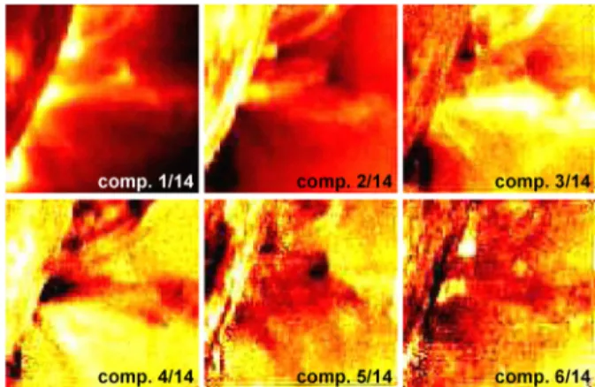
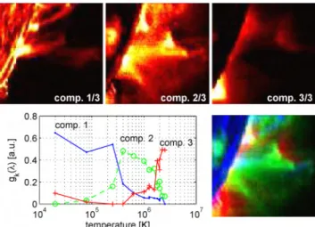
The 3 sources obtained by BPSS and their mixing co-efficients are shown in Fig. 4. In contrast to the SVD and the ICA, the BPSS identifies sources that can be linked to known processes in the solar atmosphere. Interestingly, the mixing coefficient reveal a clear temperature ordering , with the 3 components capturing emissions that respectively origi-nate from the coolest layers (1), the medium hot ones (2) and the hot corona (3). The cold component is associated with the lowest layers of the solar atmosphere, in which the solar surface comes out as a bright disk. The small loops that stand out against the dark horizon are structured by the solar mag-Fig. 3. The 6 first spatial componentsjj,(x)obtained by SVD of the data. The same colour scaling is used for all images. Except for component I, intensities are both negative and pos-itive. 14 12 6 8 10 co mponent k 4 . .. . . . ···· 0·· 2 "T L,
p"
P" ():. 0.·.:. '.'.0·' '. '.0·' ... . :0 :0:: 10-2 ,-.-~-~-~-~-~-~--'---'o
Figure 2 shows the distribution of the relative variance
Ek
=
100AU
Li
A;
of each component. The strong order-ing confirms the redundancy of the data and suggests that the salient features are expressed by 2 to 5 components only. Sim-ilar results are obtained when no Anscombe transform is ap-plied, but the ordering ofthe components then is less strong.The 6 first spatial components are shown in Fig. 3. They are not realistic because the intensities are non-positive. A deeper inspection reveals that most components actually mix different types of solar structures. A more appropriate prior would be the statistical independence of the components. Independent Component Analysis (lCA) indeed reveals a clearer picture with a better temperature ordering [4]. There A conspicuous feature in Fig. I is the high correlation be-tween the different images. There are two reasons for this. First, the same line of sight (i.e. pixel) may capture contribu-tions coming from regions with different temperatures. Sec-ond, the temperature response associated with each spectral line is generally wide, and sometimes not even unimodal.
One can reasonably assume that the intensity of each pixel is a linear mixture of a large set of pure component spectra. The number of pure spectra is much too large to extract them individually, even using a supervised method. Blind source separation, however, in which both the spectra and their mix-ture coefficients are unknown, may provide a realistic descrip-tion of the solar atmosphere.
As a first step of data processing, we compute the Singu-lar Value Decomposition (SVD) ofthe images. Each image is 85 x 87 pixels in size. We unfold the 85 x 87 x 14 data cube into a 7395 x 14 matrix by lexicographically ordering each image. In doing so, we implicitly assume that the pixel in-tensities I(x,A)
=
Lk~l Ak fk(X) gk(A) are expressed as a separable set of orthonormal spatial and wavelength com-ponents.The CDS spectrometer counts photons , and for each pixel the noise obeys a mixture of Poisson and normal laws. The variance can then be stabilised by applying the generalised Anscombe transform [3], which is equivalent here to taking the square root of the intensity. Each image is subsequently normalised to its mean value.
netic field. Particle acceleration processes can locally heat the plasma to several million degrees, leading to the hot diffuse structures that appear in component 3. An important result is that all 14 spectral lines, in spite of their differences, can be classified in 3 temperature bands only, whose properties can be inferred from the data without imposing a physical model. Our results are robust, in the sense that the same temperature ordering is obtained for other regions or events, provided all three layers are represented in the data.
...,. 0.6 OJ ~ 0.4 3:.l<: CD 0.2 105 106 temperature [K]
Fig. 4. Spatial components obtained by BPSS of the data, us-ing 3 sources (top) and their associated mixus-ing coefficients, plotted versus the characteristic emission temperature of each spectral line (bottom). Also shown (bottom right) is a mul-tispectral representation of the Sun in which component I is assigned to the blue channel, component 2 to the green chan-nel and component 3 to the red chanchan-nel. This colour figure can only be properly interpreted in the online version of the article.
A useful outcome is the possibility to condense the salient features of all 14 spectra into a single three-temperature rep-resentation of the Sun. We do so by assigning the blue, green and red channels respectively to the cold, intermediate and hot components. This multichannel repres entation of the Sun is shown in Fig. 4. We are currently adapting this representa-tion for delivering in real-time approximate temperature maps ofthe Sun based on high resolution (4kx4k) images from the future SDO satellite.
3. SECOND EXAMPLE: SPECTRAL MIXTURES Let us now consider the Sun as a point source, with high resolution UV spectra. Such spectra are important for space weather applications since different wavelengths are absorbed at different altitudes of the Earth's atmosphere. Variations in the UV flux can affect radio communications, satellite orbits (through increased air drag) and positioning by GPS.
We concentrate here on 6 years of daily measurements
made since Feb. 2002 by the SEE spectrometer onboard the TIMED satellite. This data set has been described in detail in [7]. SEE continuously measures the UV spectrum from 27 to 192.5 nm with 0.1 nm spectral bins; the instrumental resolution is 0.4 nm. Each spectral bin integrates emissions that are emitted by various spectral lines and come from all parts of the Sun. All these contributions are mixed in a linear way, so blind source separation is again justified. As in the previous section, we assume that the spectral irradiance ma-trix1(>",t)
=
LkAk f k(t ) gk(>") can be decomposed into a series of elementary spectragk(>")
with their associated mix-ing coefficients f k(t). The data are stored in a 2142 x 1546 matrix, in which columns correspond to spectral bins.140.3nm Si I
2002 2003 2004 2005 2006 2007 2008 2009 2010
year
Fig. 5. Time evolution of 4 characteristic spectral lines. The intensities have been renormalized and shifted vertically to ease comparison.
Fig. 5 shows the time evolution of 4 typical spectral lines and reveals the remarkable coherency of the solar spectrum. All spectral bins exhibit the same downward trend, which co-incides with the decaying solar cycle. On smaller time scales, however, significant differences arise. Note the conspicuous 27-day modulation that is caused by solar rotation. In a pre-vious study [7], based on SVD and multidimensional scaling, we showed that very few degrees of freedom are at play in the spectral variability.
The elementary spectra associated with the solar irradi-ance have to be positive, so we again consider BPSS. As in the previous example, there is no crisp criterion for determin-ing the number of sources. By runndetermin-ing the BPSS with dif-ferent numbers of sources, however, we find that with more than 3 sources, the method starts using instrumental artefacts to separate different contributions. That is, the signal-to-noise ratio is insufficient to allow more than 3 sources to be properly identified. Incidentally, we discovered that wayan instrumen-tal artefact that had been insufficiently corrected in the data.
The mixing coefficients fk (t )are shown in Fig. 6. The first two components and their spectra tum out to be directly associated with known solar contributions, and are further dis-cussed in [8]. The third component, however, is enigmatic as it increases while all spectral lines are decaying. Its
as-o
L-_----'_ _----L_ _---'-_ _---'-_ _--'-'---L:....l2002 2003 2004 2005 2006 2007 2008
year
Fig. 6. Time evolution of mixing coefficients obtained by ap-plying BPSS to TIMED/SEE spectra. The vertical scale is arbitrary.
sociated spectrum (not shown here) is also puzzling, since it captures emissions coming from coolest layers of the solar atmosphere. This component probably does not represent a true physical contribution to the spectra as it is sensitive to the preprocessing; it should rather be considered as a differ-ential correction.
4. CONCLUSIONS
The central result is the existence of 3 sources only for adequately describing the salient features of spectral- and spatially-resolved UV emissions from the solar atmosphere. This finding contrasts with the complexity of the underlying physical processes and confirms the remarkable structuring of the atmosphere by the solar magnetic field. The existence of three characteristic sources only had already been suggested by some [9, 10] but the BPSS for the first time provides direct quantitative evidence for it.
The sources we identify in spatial and in spectral linear mixtures are similar but not identical. Both reveal a clear tem-perature ordering, and confirm the importance of the latter. The two sets of sources, however, are not fully comparable since they are estimated from different spectral ranges.
The major advantage of such empirical methods over ex-isting physical models is the ability to perform fast data reduc-tion and deliver inputs for segmentareduc-tion schemes. They also ease the comparison between observations and the outcome of physical models. We are presently investigating whether the sources from complementary data-sets (one with spatial and one with spectral mixtures) can help improve improve the spatial or spectral resolution where it is lowest. Another field of study is the association of source separation tech-niques with multiscale analysis for improving the separation. Hot coronal regions, for example, are often diffuse, thereby providing additional leverage for the source separation proce-dure.
Acknowledgements: We gratefully thank the SoHO/CDS and the TIMED/SEE teams for delivering the excellent data that were used in this study.
5. REFERENCES
[I] M. J. Aschwanden, Physics of the Solar Corona . An
Introduction with Problems and Solutions (2nd edition),
Praxis Publishing Ltd., Chichester, UK, Dec. 2005. [2] V. Zharkova, S. Ipson, A. Benkhalil, and S. Zharkov,
"Feature recognition in solar images," Artificial
Intelli-gence Review,vol. 23, no. 3, pp. 209-266, 2005. [3] J.-L. Starck and F. Murtagh, Astronomical Image and
Data Analysis, Springer, Berlin, 2nd edition, 2006. [4] T.Dudok de Wit and F.Auchere, "Inferring
Tempera-ture from Morphology in Solar EUV Images,"
Astron-omy and Astrophysics,vol. 466, pp. 347-355,2007. [5] S. Moussaoui , D. Brie, A. Mohammad-Djafari, and
C. Carteret, "Separation negative mixture ofnon-negative sources using a bayesian approach and mcmc sampling," IEEE Transactions on Signal Processing, vol. 11, pp. 4133--4145,2006.
[6] S. Moussaoui , H. Hauksdottir, F. Schmidt, C. Jutten, J. Chanussot, D. Brie, S. Doute, and J. A. Benedikts-son, "On the decomposition of Mars hyperspectral data by ICA and Bayesian positive source separation,"
Neu-rocomputing,vol. 71, no. 10-12, pp. 2194-2208, 2008. [7] T.Dudok de Wit, J. Lilensten, J. Aboudarham, P.-o.
Amblard , and M. Kretzschmar, "Retrieving the solar EUV spectrum from a reduced set of spectral lines,"
An-nales Geophysicae,vol. 23, pp. 3055-3069, Nov. 2005. [8] P.-O. Amblard, S. Moussaoui, T. Dudok de Wit, J. Aboudarham, M. Kretzschmar, J. Lilensten, and
F.Auchere , "The EUV Sun as the superposition of ele-mentary Suns," Astron. Astroph. , vol. 487, pp. L13-L 16, Aug. 2008.
[9] J. L. Lean, W. C. Livingston, D.F.Heath, R. F. Don-nelly, A. Skumanich , and o. R. White, "A three-component model of the variability of the solar ultra-violet flux 145-200 nm," 1.Geophys. Res., vol. 87, pp. 10307-10317, Dec. 1982.
[10] U. Feldman and E. Landi, "The temperature structure of solar coronal plasmas," Physics ofPlasmas, vol. 15, no. 5, pp. 056501, May 2008.