Quantification of the specific yield in a two-layer hard-rock aquifer model

HAL Id: hal-01537837

https://hal.sorbonne-universite.fr/hal-01537837

Submitted on 13 Jun 2017

HAL is a multi-disciplinary open access archive for the deposit and dissemination of sci-entific research documents, whether they are pub-lished or not. The documents may come from teaching and research institutions in France or abroad, or from public or private research centers.

L’archive ouverte pluridisciplinaire HAL, est destinée au dépôt et à la diffusion de documents scientifiques de niveau recherche, publiés ou non, émanant des établissements d’enseignement et de recherche français ou étrangers, des laboratoires publics ou privés.

hard-rock aquifer model

Véronique Durand, Véronique Léonardi, Ghislain de Marsily, Patrick

Lachassagne

To cite this version:

Véronique Durand, Véronique Léonardi, Ghislain de Marsily, Patrick Lachassagne. Quantification of the specific yield in a two-layer hard-rock aquifer model. Journal of Hydrology, Elsevier, 2017, 551, pp.328-339. �10.1016/j.jhydrol.2017.05.013�. �hal-01537837�

Quantification of the specific yield in a two-layer hard-rock

1

aquifer model

2

Véronique Durand

(1)

, Véronique Léonardi

(2)

, Ghislain de Marsily

(3)

, Patrick

3

Lachassagne

(4) 4

(1) Laboratoire GEOPS; Univ. Paris-Sud; CNRS, UMR 8148; Bât. 504, 91405 Orsay Cedex, France; 5

veronique.durand@u-psud.fr 6

(2) Laboratoire Hydrosciences; Université de Montpellier; CNRS, UMR 5569; CC57, 163 rue Auguste 7

Broussonet, 34090 Montpellier, France; veronique.leonardi@umontpellier.fr 8

(3) Laboratoire Metis; Sorbonne Universités, UPMC Univ. Paris 06; CNRS, UMR 7619; EPHE; 4 place 9

Jussieu, 75005 Paris, France; gdemarsily@aol.com 10

(4) Water Institute by Evian, Danone Waters, Evian-Volvic World, BP 87, 74500 Evian-les-Bains Cedex, 11

France; patrick.lachassagne@danone.com 12

Abstract

13

Hard Rock Aquifers (HRA) have long been considered to be two-layer systems, with a mostly 14

capacitive layer just below the surface, the saprolite layer and a mainly transmissive layer 15

underneath, the fractured layer. Although this hydrogeological conceptual model is widely accepted 16

today within the scientific community, it is difficult to quantify the respective storage properties of 17

each layer with an equivalent porous medium model. Based on an HRA field site, this paper attempts 18

to quantify in a distinct manner the respective values of the specific yield (Sy) in the saprolite and the 19

fractured layer, with the help of a deterministic hydrogeological model. The study site is the 20

Plancoët migmatitic aquifer located in north-western Brittany, France, with piezometric data from 36 21

observation wells surveyed every two weeks for eight years. Whereas most of the piezometers (26) 22

are located where the water table lies within the saprolite, thus representing the specific yield of the 23

unconfined layer (Sy1), 10 of them are representative of the unconfined fractured layer (Sy2), due to 24

their position where the saprolite is eroded or unsaturated. The two-layer model, based on field 25

observations of the layer geometry, runs with the MODFLOW code. 81 values of the Sy1/Sy2 26

parameter sets were tested manually, as an inverse calibration was not able to calibrate these 27

parameters. In order to calibrate the storage properties, a new quality-of-fit criterion called "AdVar" 28

was also developed, equal to the mean squared deviation of the seasonal piezometric amplitude 29

variation. Contrary to the variance, AdVar is able to select the best values for the specific yield in 30

each layer. It is demonstrated that the saprolite layer is about 2.5 times more capacitive than the 31

fractured layer, with Sy1=10% (7%<Sy1<15%) against Sy2=4% (3%<Sy2<5%), in this particular 32

example. 33

Keywords

34

Hard-rock aquifer; Specific yield; Two-layer numerical model; Quality-of-fit criterion 35

Highlights

36

- Quantitative evidence that the saprolite layer is more capacitive than the fractured one 37

- New quality-of-fit criterion, AdVar, based on the piezometric amplitude variations 38

1

Introduction

39

Hard-Rock aquifers (HRA) have long been considered to be two-layer systems, with (i) a weakly 40

transmissive but rather capacitive layer (with a high specific yield) just below the surface, the 41

unconsolidated weathered layer (also called the saprolite here, or the regolith) and (ii) a more 42

transmissive but less capacitive layer underneath, the fractured layer. This hydrogeological 43

conceptual model is now widely accepted in the scientific community (see for instance Chilton and 44

Foster, 1995; Cho et al., 2003; Dewandel et al., 2006; Dewandel et al., 2011; Lachassagne et al., 2011; 45

McFarlane, 1992; Taylor and Howard, 1999, 2000; Wright, 1992). These two layers belong to the 46

HRA weathering profile and reach, in general, a thickness that may exceed 100 m (Lachassagne et al., 47

2011). At the watershed scale, the hydrodynamic storage and flow properties of the underlying 48

unfractured rocks (basement) are negligible. The capacitive (or storage) properties of this two-layer 49

system, namely its storativity, or specific yield Sy where the aquifer is unconfined, were first studied 50

and characterized to gain a better estimate of the long-term groundwater storage available in HRAs. 51

It was established early on that the fractures in HRAs are well connected (Lenck, 1977) and later, that 52

this fractured layer could be considered a continuous aquifer (Guihéneuf et al., 2014; Lachassagne et 53

al., 2001). Some studies have focused on the specific yield of the saprolite layer, and consequently

54

on the capacitive role it can play during withdrawals (Detay et al., 1989; Howard and Karundu, 1992; 55

Rushton and Weller, 1985). The processes controlling the development of these two layers are 56

increasingly well understood and the ways to define their respective geometry and thickness are 57

more precise (Dewandel et al., 2006; Lachassagne et al., 2011; Wyns et al., 2004); moreover, 58

pumping test methods to characterize their hydrodynamic properties at the borehole scale have 59

been improved (Maréchal et al., 2004). However, the precise determination of the respective 60

storage properties of each layer remains an issue, particularly at the watershed scale (Dewandel et 61

al., 2012).

62

A number of authors have modelled these systems as equivalent porous media, but none of them 63

has managed to calibrate the specific yield of both layers simultaneously. Gupta et al. (1985) used a 64

single-layer model, considering that both layers were interconnected. Ahmed et al. (2008) presented 65

a two-layer model calibrated on an Indian site, but unfortunatly the saprolite layer was always 66

unsaturated, which made it impossible to calibrate its specific yield. An interesting specific yield 67

calibration for a two-layer model of an HRA is presented in Lubczynski and Gurwin (2005), but the 68

paper did not focus on this parameter, so that the specific yield values were not presented, nor the 69

potential differences between the saprolite and the fractured layer. The authors point out the 70

difficulty in calibrating the specific yield with an automatic inverse method like PEST, and prefer a 71

trial-and-error calibration, in order to "have the best fit of the pattern of rises and recessions of the 72

groundwater table". The same kind of difficulty was also highlighted by Mazi et al. (2004), where to

73

calibrate the specific yield, the authors needed the help of an expert as a complement to the 74

automatic calibration. In fact, automatic calibration methods are mainly focused on the hydraulic 75

conductivities, adjusted with the help of a quality-of-fit criterion based on the differences between 76

the modelled and observed hydraulic heads (Carrera et al., 2005; de Marsily et al., 2000; Zhou et al., 77

2014). For aquifer management purposes, a correct quantification of the distinct specific yields of 78

the two layers is important, as a potentially highly capacitive layer represented by the saprolite may 79

sustain the exploited water resources in the fractured layer. 80

In this context, the main objective here is to calibrate the specific yield in each of the two layers of a 81

finite-difference hydrogeological model, at the watershed scale. This parameter, representative of 82

the storage properties, is crucial in groundwater management purposes. Because of the difficulties 83

mentioned above, this calibration required the development of a new quality-of- fit criterion. This 84

study uses field data from an HRA in Brittany, France, described in the following section. The model 85

is then presented, followed by the calibration (approach and results). The results are discussed, and 86

a conclusion summarizes the main results of the study. 87

2

Geology and hydrogeology of the study site

88

2.1 General presentation 89

The studied site (Durand et al., 2006) is located in north-eastern Brittany, France, 10 km from the 90

English Channel shoreline (Figure 1), in a landscape of grass-land, forest and farmland, with a smooth 91

relief. In the middle of the studied site stands a 90 m ASL hill, surrounded by the Arguenon River at 92

10 m ASL flowing toward the English Channel (Figure 1). The migmatites that constitute the rocks in 93

this area belong to the Saint-Malo dome, exhumed at the end of the Cadomian Orogeny (540 Ma). 94

These partially melted rocks originated from detrital sediments interbedded with graphitic cherts, 95

composed of quartz. They now form a folded gneiss with relict bands of cherts. They were later 96

intruded by dolerite dykes during the Hercynian period (330 Ma). The associated hard-rock aquifer is 97

located mostly in the sub-surface stratiform weathered layers (Durand et al., 2006), which consist of: 98

(i) a cover of unconsolidated weathered rocks (saprolite), several tens of meters thick where it has 99

been preserved from erosion, consisting mainly of clay or sandy clay, that are the weakly permeable 100

transformation products of the initial minerals; (ii) beneath this layer, and above the unweathered 101

bedrock, a fractured layer, some 50 m thick or more, resulting from rock shattering under the 102

influence of stress generated by the swelling of certain minerals during the early stages of 103

weathering (Dewandel et al., 2006; Lachassagne et al., 2011; Wyns et al., 2004). Field surveys and 104

geophysical mapping of the two weathered-fractured layers and of the various geological 105

heterogeneities, such as graphitic cherts and dolerite dykes, are described in a previous study 106

(Durand et al., 2006). In an area covering only 4 km², six pumping wells and 36 piezometers (Error! 107

Reference source not found.), owned and monitored by the Nestlé Waters Company for bottled 108

natural mineral and spring water, provide an unusually rich set of hydrogeological data. While most 109

piezometers (26) are located where the saprolite is saturated, and will thus help to quantify the 110

storage in this layer, 10 of them are located where the saprolite is either eroded, or unsaturated, and 111

will consequently help the storage quantification in the fractured layer. 112

113

Figure 1. Location of the study area (within the grey-shaded polygon), the meteorological

114

stations (stars), and the only gauging station (square)

115

116

Figure 2. Geometry of the finite-difference model, boundary conditions, thickness of layer 1

117

(white: zero thickness) and location of the piezometers with their respective numbers

118

119

2.2 Recharge estimation 120

The daily rainfall was measured directly at the Plancoët bottling plant (Figure 1). The mean annual 121

rainfall (R) is on average 800 mm, with a typical oceanic climate. Around Plancoët, three weather 122

stations belonging to Météo France, located in Pleurtuit, Quinténic and Trémeur (Figure 1), also 123

provided data on rainfall and daily potential evapotranspiration (PET) estimated with Penman’s 124

relation (Penman, 1948). Daily river flow measurements were available at the Jugon-les-Lacs gauging 125

station (Figure 1) on the Arguenon River, which drains the studied area. Over the eight years of the 126

monitored period, a mean annual river discharge of 253 mm/y was found at the Jugon-les-Lacs 127

gauging station, for the area of its catchment (see Durand (2005) for more details). Thornthwaite’s 128

method (Castany, 1967; Maidment, 1993; Vittecoq et al., 2010) was used at a daily time step and 129

during the eight-year monitored period to compute the effective rainfall (EffR), equal to P minus Real

130

EvapoTranspiration (RET), or to the sum of the aquifer recharge plus the surface runoff over the 131

catchment. The computation used the rainfall data measured directly on the Plancoët site, and the 132

weighted average of PET data from the three Météo France weather stations calculated for the site. 133

The maximum soil storage capacity (MSC), the parameter used in Thornthwaite’s method to 134

temporarily store rainfall in the soil before it is taken up by RET and EffR, was calibrated so that the

135

EffR value would be as close as possible to the available annual catchment flow in the area. In this

136

hydrogeological context, both runoff and aquifer recharge reach the river in a year (Molénat et al., 137

1999). Rounding off the value, the best fit for MSC was obtained with 100 mm, leading to a mean 138

real evapotranspiration of 530 mm/y and an annual effective rainfall of 247 mm/y, quite close to the 139

average river discharge. Figure 3 presents the meteorological data (P, RET and EffR) averaged for

140

each model time step in mm/day. It shows that EffR is positive only during the winter season, when 141

RET is sufficiently low. Considering the landscape, smooth relief and grassy hills, the field 142

observations during the winter rainy season (no runoff observed even during the most intense rainy 143

periods), and for simplicity reasons, the recharge was fixed at 100% EffR. This will be discussed in the

144

final discussion part below. 145

146

Figure 3. Precipitation (P), calculated real evapotranspiration (RET) and effective rainfall

147

(Eff

R

) used for each model time-step

148

2.3 Water table variations 149

The piezometric signals in this type of aquifer, in a temperate climate, have a pseudo-sinusoidal 150

shape with an annual period, where the highest levels are observed at the end of winter and the 151

lowest at the end of summer. The amplitude of the head variations between the high and low levels 152

depends both on the time distribution of the recharge and on the Sy values (Maréchal et al., 2006). 153

As the specific yield plays an active role only for an unconfined layer, it is either Sy in the saprolite 154

layer 1 (Sy1) or Sy in the fractured layer 2 (Sy2) that is effective, depending on the piezometer 155

location: Sy1 is effective where layer 1 (saprolite layer) is present and saturated (26 piezometers), 156

and Sy2 will be effective where layer 1 has been eroded or is unsaturated (10 piezometers). In the 157

data set, both piezometer types are well represented, and it is interesting to compare the signals 158

obtained for each type. The piezometric head was measured manually in each observation hole from 159

1/1/1996 to 30/11/2003, with a time step of approximately 15 days. From these data, one can see 160

that the mean annual amplitude variation of the piezometric levels is higher in the piezometers 161

representing layer 2, the fractured layer (6.1 ± 2.3 m in average) than in those representing layer 1, 162

the saprolite (3.4 ± 1.3 m in average). An example is shown in Figure 4. 163

164 165

Figure 4. Measured water table in two types of piezometers: P17 in the fractured layer and

166

P26 in the saprolite

167

3

Model description

168

The finite-difference PMWIN model (Chiang and Kinzelbach, 2000) that uses the MODFLOW code 169

(Harbaugh and McDonald, 1996) was chosen for this work. The model was built with two parallel 170

layers in order to account for the assumed distinct hydrodynamic properties of the saprolite (layer 1), 171

and the underlying weathered fractured layer (layer 2). 172

The geometry of each of these layers (shape of top and bottom) was determined by extensive field 173

work over the entire 116 km² study area (Durand et al., 2006). The maximum thickness of layer 2, 174

where it is totally preserved from erosion, was found to be quite uniform across the studied area and 175

was estimated at 100 m, a thickness consistent with our experience of the Brittany geology and the 176

available borehole logs and geophysical data (Durand, 2005). Layer 2 is present over the whole 177

modelled area (116 km²), as it has never been totally eroded, whereas layer 1, with a maximum 178

thickness of 40 m, covers only 54 km², due to local patches of total erosion (Error! Reference source 179

not found.). 180

In the centre of the modelled area, owned by Nestlé Waters and including the bottled-water 181

exploitation zone, the accuracy of the structural map and the number of hydrogeological data are 182

much higher than in the other areas. The rectangular grid of the model (Error! Reference source not 183

found.) is therefore a compromise between good precision where the data are dense and relatively 184

fast calculations: consequently, the width of the rectangular model cells varies from 400 m on the 185

borders to 40 m in the exploitation zone. Each of the two layers is modelled vertically by a single cell 186

whose height is equal to the thickness of the corresponding layer. The layers are connected 187

vertically, as they are assumed to be in reality. Layer 1 is modelled as an unconfined aquifer and 188

layer 2 can be either confined or unconfined, depending on the potential lowering of the piezometric 189

head below the bottom of layer 1. 190

The simulations were performed in a transient flow regime which allowed the time-dependent 191

seasonal and yearly piezometric variations observed in the aquifer to be reproduced. The modelling 192

runs from 1/1/1996 to 30/11/2003, with a time step of 15 days, similar to the frequency of the 193

piezometric head measurements. 194

Six pumping wells in the exploitation zone (Error! Reference source not found.) are used for bottled-195

water production and their time-varying discharges are precisely recorded and used in the model. 196

No other significant pumping is known to occur in the whole modelled domain, except a few tens of 197

litres per day, in the summer, from shallow wells, not considered in this study. 198

The total modelled domain, chosen much larger than the area exploited by the bottling plant, is 199

limited by permanent rivers, considered to be prescribed-head boundaries, so no conductance 200

parameter was set for these cells (Error! Reference source not found.). The river elevations were 201

extracted from the 1/25 000 topographic map of the area (IGN, 2000) assuming a linear slope 202

between known points (contour lines every 5 m). In the exploitation zone, the topographic 203

depression due to a disused quarry of graphitic cherts located near the top of a hill is at the origin of 204

a small perennial lake (Error! Reference source not found.). The level of this lake, generally higher 205

than that of the observed nearby piezometric levels, shows that it functions as an infiltration zone. It 206

is modelled as a reservoir in the MODFLOW code (Error! Reference source not found.), with a 207

prescribed constant level, a water depth of 1 m, and an underlying 1 m-thick sediment layer with a 208

vertical hydraulic conductivity of 1.2 10-5 m/s. This value was calibrated so that the infiltration from 209

the lake is consistent with its hydrological balance. Two small temporary rivers (Error! Reference 210

source not found.) surrounding the hill are considered as drains in the model, because they drain the 211

aquifer during high-water periods and are dry during the rest of the year. A calibrated hydraulic 212

conductance of 5.8 10-4 m2/s was assigned to the contact area between the aquifer and these drains. 213

The initial value of the piezometric heads on January 1st_{, 1996 was estimated as follows: a}

214

preliminary run of the model over the whole 8-year period started with heads at the ground surface; 215

the calculated heads on November 3rd, 2003 at the end of this preliminary run were then taken as the 216

initial conditions for January 1st_{, 1996.}

217

4

Calibration

218

4.1 Homogeneous model calibration 219

In this type of aquifer, the hydraulic conductivity might be very heterogeneous; but the 220

heterogeneity does not depend primarily on the geometry of the two layers, but rather on the 221

location of fractures and other spatial discontinuities. As this type of heterogeneities was not the 222

main focus here, a homogeneous hydraulic conductivity was chosen for each layer, and the PEST 223

automatic calibration method in transient state (Doherty, 2004), within the PMWIN interface, was 224

used to provide the best possible average fit. In a first approximation, the hydraulic conductivity and 225

the specific yield, considered here to be uniform in space and identical for the two layers, were 226

calibrated simultaneously: the best calibrated hydraulic conductivity was 8.1 10-7 m/s, and the 227

specific yield was 6 %. An arbitrary value of the storage coefficient for the confined layer was set at 228

10-4. As the hydraulic conductivity is only roughly calibrated on the whole model, the simulated 229

heads are therefore shifted locally, as compared to the observed ones. It is considered that this shift 230

does not influence the further calibration of Sy1 and Sy2, based on a good amplitude variation fit. 231

This specific point is discussed in the final discussion part of the article. 232

4.2 Classical calibration of the specific yield using the variance criterion 233

In a second step, a model with distinct storage properties in the two layers was used to obtain a 234

better calibration of the specific yield (Sy). This hydraulic parameter may be considered the most 235

important one in the two-layer model. Contrary to the hydraulic conductivity, which influences the 236

average hydraulic heads, this parameter influences primarily the amplitude of the hydraulic-head 237

variations. We used PEST for an automatic calibration of Sy1 and Sy2, fixing the previously calibrated 238

value for the hydraulic conductivity. Sy1 was found to be optimum at 3%, but the Sy2 calibrated 239

values were always the maximum defined ones, even when amounting to 50%. This can be explained 240

by the fact that, due to the imperfect calibration of the hydraulic conductivity of the model, the 241

average simulated head values are shifted as compared to observed data, and that the quality-of-fit 242

criterion used in PEST is the least squares of the differences between modelled and observed heads. 243

As a high Sy tends to reduce the amplitude variation of the signal, the quality-of-fit criterion is better 244

with a "flat" signal than a varying one in the case where the general average is very different from 245

the true one. In order to understand the automatic calibration process, and to quantify the 246

performance of each model, various combinations of Sy parameters were tested manually. Nine 247

values of Sy1 and Sy2 were thus tested (1%, 2%, 3%, 4%, 5%, 6%, 7%, 10% and 15%), leading to 81 248

model runs. The classical head squared deviation variance (Var, Equation 1) between the calculated 249

(calcd) and observed heads (obsd) on each measurement day of the data set was calculated for all 36

250

piezometers and this variance was averaged over the whole data set for each model. 251

ar nd al d-o sd

n (1)

252

with n the number of data points for each piezometer. 253

Note that in PEST, the sum of squared deviation is used, but here we take into account the number 254

of measurements over periods of varying lengths in order to compare the results obtained for each 255

piezometer. Considering all piezometers, the best Var value was 97 m² for Sy1=3% and Sy2=15%. 256

Nevertheless, it appeared that these statistics might be biased by the fact that some simulated heads 257

concerned another layer than the one of the observed data (for instance, the observed piezometry is 258

in the saprolite while the computed one is in the fractured layer, or vice-versa). As the hydraulic 259

conductivity was not calibrated, this was observed on 7 piezometers representative of the saprolite, 260

and on 4 from the fractured layer. In order to avoid this specific bias and improve the results, we 261

chose to remove these piezometers and re-calculate the average Var values. The results obtained for 262

the various Sy values are given in matrix form (Table 1), the values of Var are shown with Sy1 values 263

in columns and Sy2 values in rows. The minimum Var values are highlighted (corresponding to the 264

better fit). Table 1 shows that the coloured cells are below the diagonal matrix, i.e. for Sy2>Sy1, and 265

that the maximum chosen Sy2 value (15% here) leads to the better Var value. This confirms that, for 266

the same reasons as explained above, the Var criterion, or any criterion based on squared head 267

deviations, as in PEST, is not appropriate for the calibration of Sy. It is therefore necessary to 268

develop another criterion better adapted to calibrate Sy in each layer. 269

270

Table 1. Var values (in m²) obtained for all Sy1 and Sy2 values. Yellow: minimum values;

271

orange, red and light brown respectively: classes around the minimum, with an increase of

272

Var of 5% of the total variation range between two successive classes

273

274

4.3 New calibration of the specific yield taking the amplitude variation into account 275

To better fit the specific yield, a new performance criterion, named "AdVar", was developed, based 276

on the seasonal piezometric amplitude variations. For each piezometer, and for each available 277

measurement on day d, a moving interval of one year after d was defined both for the observed and 278

the calculated heads. Then for that one-year interval, each piezometer amplitude-deviation variance 279

AdVar is defined as the average of the squared amplitude deviations, i.e.: 280 d ar ma al d-min al d - ma o sd-mino sd nday d nday (2) 281

with maxcalcd, mincalcd, maxobsd, minobsd respectively the maximum-minimum values of the calculated

282

and observed heads over the one-year interval after day d, and nday the number of measurement

283

dates d available, i.e. the total number of data points less those of the last year of data. Like the 284

variance, AdVar is always positive and the smaller values indicate a better fit. For a better 285

visualisation of the AdVar behaviour compared to Var, when quantifying the fit between theoretical 286

sinusoidal curves, please refer to Appendix 1. 287

Considering all piezometers, the best AdVar value was 9.7 m² for Sy1=10% and Sy2=4%. Removing 288

the biased piezometers as previously, and re-calculating the average AdVar values, the same matrix 289

form as for Var was used for AdVar in 2, with Sy1 values in columns and Sy2 values in rows. 2 shows 290

that the coloured cells are above the diagonal matrix, i.e. for Sy1>Sy2, with AdVar, which seems 291

more realistic from a hydrogeological viewpoint than the results obtained with Var. Following this 292

criterion, the specific yield is about 10% in the saprolite (Sy1) and 2% in the fractured layer (Sy2). The 293

uncertainty intervals are 7%<Sy1<15% and 1%<Sy2<3%. 294

295

Table 2. AdVar values (in m²) obtained for all Sy1 and Sy2 values. Yellow: minimum values;

296

orange, red and light brown respectively: classes around the minimum, with an increase of

297

AdVar of 0.5% of the total variation range between two successive classes

298

299 300

4.4 Comparison of the simulated water tables from the best adjustments of Var and AdVar 301

To give a better view of the results obtained in each of the two layers of the model, Figure 5 shows 302

the observed piezometric variations compared with two simulations in P26, a piezometer 303

representative of the saprolite layer, and in P17, representative of the fractured layer. The first 304

model, with Sy1=2% and Sy2=15%, corresponds to the best performance for the Var criterion, and 305

the second model, with Sy1=10% and Sy2=2%, to the best performance for the AdVar criterion. 306

Even if the hydraulic conductivity, and thus the mean value of the piezometric head is not perfectly 307

fitted, the second model with the lowest Sy2 and the highest Sy1 better mimics the observed 308

amplitude variations than the first one, with low Sy1 and high Sy2 values. 309

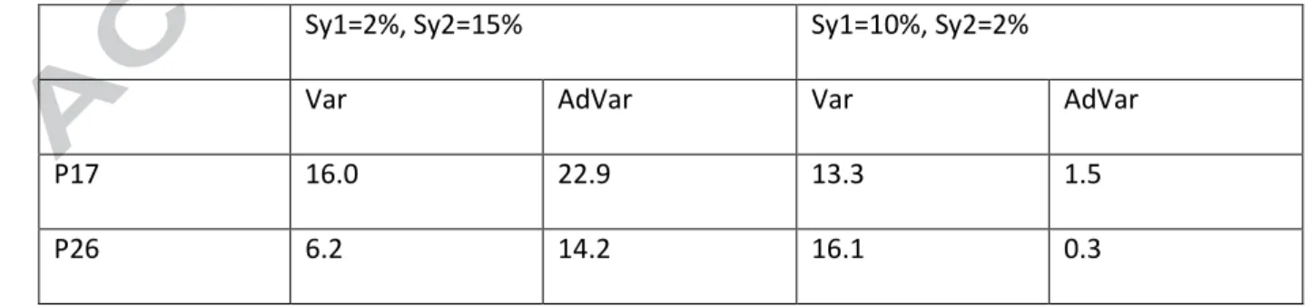
The Var and AdVar values are given in Table 3 for each of these piezometers with the two above 310

models. Except for Var in P17, the values follow the same trend as the average Var and AdVar 311

values: the first model gives a better Var, and the second a better AdVar. Between two distinct 312

models, an expert eye would choose in accordance with the AdVar criterion, not with the Var one. 313

As a conclusion to this part of the work, the obtained calibration of Sy can be considered very 314

satisfactory, particularly when one considers that, for this study, no spatial variations neither of the 315

hydraulic conductivity, nor of the specific-yield, were considered. 316

317

Figure 5. Examples of piezometric variations for P26 within the saprolite and P17 within the

318

fractured layer. Two model results corresponding to the best Var and AdVar values are

319

compared to the observed data

320

Table 3. Var and AdVar values (in m²) for piezometers P26 and P17 with two Sy set of values

321

Sy1=2%, Sy2=15% Sy1=10%, Sy2=2%

Var AdVar Var AdVar

P17 16.0 22.9 13.3 1.5

5

Discussion

322

5.1 Comparison of specific yield values with other studies 323

These results of specific yield values are consistent with the conceptual model developed by 324

Lachassagne et al. (2001) and Dewandel et al. (2010), notably with a decrease of Sy with depth. The 325

obtained Sy values (Sy1=10% and Sy2=4% for the best AdVar values) are higher than those given by 326

Rushton and Weller (1985) for a granite in India and by Compaore et al. (1997) for a granite in 327

Burkina Faso. These authors estimated the specific yield of the saprolite layer at between 1 and 2%. 328

Nevertheless, as shown by Wyns et al. (2004), Sy in the saprolite is sensitive to the type of lithology: 329

for instance, Sy increases with the coarsening of the minerals of the parent rock and also with the 330

quartz content. The interval of specific-yield values measured by Wyns et al. (2004) on several types 331

of hard-rock lithologies in Brittany (France) includes the values estimated in the present study. 332

5.2 Recharge sensitivity 333

In order to simplify the results, the recharge value was fixed arbitrarily in this study, considering that 334

runoff is negligible. Previous work done elsewhere in Brittany (Durand and Juan Torres, 1996; 335

Jiménez-Martinez et al., 2013; Molénat et al., 1999) using other methods, such as isotope and 336

natural tracer analyses, river discharge recession-curve analysis, or temporal groundwater head 337

variations in response to recharge inputs, has arrived at similar conclusions. Nevertheless, it is 338

possible to explore the sensitivity of the model to the recharge, testing various recharge values. 339

Figure 6 shows the observed and simulated heads at P26, for the reference model (Sy1=10%, 340

Sy2=4%, Recharge=100% EffR), and for two other models, keeping the same Sy values, and testing

341

Recharge=70% EffR and Recharge=30% EffR. Note that the simulated heads with low recharge values

342

never stop decreasing from the beginning to the end of the simulation, and even drop below the 343

observed values. They also decrease a little with the maximum recharge, due to a problem in the 344

initial head, difficult to calibrate here, but it appears that the average heads tend to stabilize at the 345

end of the modelled period. It is not the case with lower recharge values, leading to the conclusion 346

that these values are too low to provide enough water to the aquifer, compared to the real natural 347

discharge and pumping rate on the site. Some graphics showing the Var and AdVar results with a 348

complete parameter set (8 recharge values for each Sy combination) are presented in Appendix 2. 349

350

Figure 6. Observed and modelled heads for P26, testing various recharge values

351

5.3 Hydraulic conductivity sensitivity 352

In this study, an arbitrary choice was made to leave out the hydraulic conductivity calibration. 353

Although it is the main parameter of the flow budget within the aquifer, this choice was made in 354

order to focus attention on the storage parameter, a crucial parameter in HRA to quantify the 355

exploitable water resources. The aim was to quantify the specific-yield in the two layers of an HRA, 356

highlighting their differences, and not to build a fully calibrated model for water-resource 357

management purposes. A local adjustment of hydraulic conductivities may induce some minor 358

modification of the temporal head amplitude variations. This is shown in Figure 7 with the example 359

of P26: the reference model (black plain line), with K=8.1 10-7 m/s, is compared to models with K=8.1 360

10-6 m/s (light grey) and K=1.2 10-7 m/s (dark grey). Changes of K highly influence the mean 361

interannual piezometric values, but influence in a minimal way the amplitude variations. One can 362

conclude that more reasonable changes in K than those of this sensitivity analysis, to better fit the 363

local data, would not seriously impact the amplitude variations. It is considered that, in the high-364

density data zone where the piezometers are located, the amplitude variations would not be much 365

affected, as the chosen homogenous K value is already quite well fitted. It is possible, however, that 366

the calibrated Sy values for both layers might not be quite exact, due to the local K variations. But 367

the general tendency toward a higher storage capacity in the saprolite layer than in the fractured one 368

will stay the same, whatever the local K values. 369

370 371

Figure 7. Observed and modelled heads on P26, testing various K values

372

5.4 Synthesis

374

Figure 8 synthesises these results in a qualitative way, presenting the respective behaviours of the 375

saprolite and the fractured layer in two columns. In the case where the water table stays in the 376

saprolite layer (first column), the observed water table (dotted blue line) varies with a low amplitude. 377

The model M1 (in orange), with a high specific yield, well reproduces this low amplitude variation, 378

but presents a computed average head value different from the observed one (lower here), as a 379

consequence of the imperfect K calibration. Therefore, the variance calculated between the M1 380

computed red curve and the observed data is high, whereas the AdVar criterion is very good. Still in 381

the first column, the inverse is shown for the model M2 (in green), with a low specific yield: its 382

amplitude variation is too high compared to the observed data, leading to a high AdVar criterion. But 383

as M2 presents an average value very similar to the observed data, the variance is better than for 384

M1. This first column shows a higher efficiency of the Advar quality-of-fit criterion (rather than the 385

Variance) in identifying the best Sy (here M1 with a high Sy), even if the average head is not well 386

calibrated (for instance because of a locally imperfect calibration of K). Inversely, in the case where 387

the water table stays in the fractured rock (second column), the observed water table varies with a 388

high amplitude. The same M1 model as previously, well fitted for the average head, shows here a 389

good variance criterion, but a weak AdVar criterion. And the same M2 model as previously, with a 390

distinct average head but an amplitude variation similar to the data, shows a weak variance but a 391

good Advar criterion. Again, this second column shows a greater efficiency of the Advar quality-of-fit 392

criterion in identifying the best Sy (here M2 with a low Sy). This emphasises that the ideal model 393

combines M1 and M2, with a relatively high specific yield in the saprolite layer, and a lower specific 394

yield in the fractured layer, which are the two main conclusions of this paper. Moreover, the AdVar 395

criterion is better adapted to quantifying the amplitude variation (thus to fit the specific yield) than 396

the Var criterion. 397

398 399

Figure 8. Schematic view of the main results showing the observed and simulated piezometric

400

amplitude variation for the two cases of a water table in the saprolite and in the fractured

401

layer.

402 403

6

Conclusion

404

In this study, a hard-rock aquifer system in Britany (France) was simulated with a two-layer 405

deterministic hydrogeological model at the catchment scale, each layer representing a specific 406

weathering horizon (saprolite and fractured layer). The storage capacities of each layer can be 407

quantified thanks to a rich data set, with piezometers representing the two types of layers, when 408

unconfined. The specific yield values are calibrated using a new quality-of-fit criterion, AdVar, based 409

on the seasonal piezometric amplitude variations. The saprolite layer is proved to be more capacitive 410

than the fractured layer, with a calibrated specific yield 2.5 times greater than that of the fractured 411

layer: Sy1=10% (7%<Sy1<15%) against Sy2=4% (3%<Sy2<5%), in this particular example. 412

Aknowlegdment

413

We are grateful to the Nestlé Waters Company for financial support from 2002 to 2005 and for 414

making the data available. 415

References

416

Ahmed, S., J.-C. Maréchal, E. Ledoux, and G. de Marsily (2008), Groundwater modelling in hard-rock 417

terrain in semi-arid areas: experience from India, in Hydrological Modelling in Arid and Semi-Arid 418

Areas, edited by H. Wheater, S. Sorooshian and K. D. Sharma, International Hydrology Series,

419

Cambridge University Press, Cambridge, UK, p. 157-189. 420

Carrera, J., A. Alcolea, A. Medina, J. Hidalgo, and L. J. Slooten (2005), Inverse problem in 421

hydrogeology, Hydrogeology Journal, 13, 206-222, doi: 10.1007/s10040-004-0404-7. 422

Castany, G. (1967), Traité pratique des eaux souterraines, Dunod ed., 661 p., Paris. 423

Chiang, W. H., and W. Kinzelbach (2000), 3D-Groundwater Modeling with PMWIN – A Simulation 424

System for Modeling Groundwater Flow and Pollution, 346 p., Berlin Heidelberg New York. 425

Chilton, P. J., and S. S. D. Foster (1995), Hydrogeological Characterisation And Water-Supply Potential 426

Of Basement Aquifers, Tropical Africa Hydrogeology Journal, 3, 36-49. 427

Cho, M., K. M. Ha, Y.-S. Choi, W. S. Kee, P. Lachassagne, and R. Wyns (2003), Relationships between 428

the permeability of hard-rock aquifers and their weathered cover based on geological and 429

hydrogeological observations in South-Korea, paper presented at IAH Conference on 430

"Groundwater in fractured rocks", Prague, 15-19 September 2003.

431

Compaore, G., P. Lachassagne, T. Pointet, and Y. Travi (1997), Evaluation du stock d'eau des altérites. 432

Expérimentation sur le site granitique de Sanon (Burkina-Faso), paper presented at Hard Rock 433

Hydrosystems, IAHS, Rabat, may 1997.

434

de Marsily, G., J.-P. Delhomme, A. Coudrain-Ribstein, and M. A. Lavenue (2000), Four decades of 435

inverse problems in hydrogeology, in Theory, Modeling, and Field Investigation in Hydrogeology: A 436

Special Volume in Honor of Shlomo P. Neuman’s 60th Birthday, edited by D. Zhang and C. L.

437

Winter, Geological Society of America Special Paper, Boulder, Colorado, p. 1-17. 438

Detay, M., P. Poyet, Y. Emsellem, A. Bernardi, and G. Aubrac (1989), Influence du développement du 439

réservoir capacitif d'altérites et de son état de saturation sur les caractéristiques 440

hydrodynamiques des forages en zone de socle cristallin, Comptes rendus de l'Académie des 441

Sciences de Paris, Série II a, 309, 429-436.

442

Dewandel, B., P. Lachassagne, R. Wyns, J.-C. Maréchal, and N. S. Krishnamurthy (2006), A generalized 443

3-D geological and hydrogeological conceptual model of granite aquifers controlled by single or 444

multiphase weathering, Journal of Hydrology, 330, 260-284, doi: 10.1016/j.jhydrol.2006.03.026. 445

Dewandel, B., P. Lachassagne, F. K. Zaidi, and S. Chandra (2011), A conceptual hydrodynamic model 446

of a geological discontinuity in hard rock aquifers: Example of a quartz reef in granitic terrain in 447

South India, Journal of Hydrology, 405, 474-487, doi: 10.1016/j.jhydrol.2011.05.050. 448

Dewandel, B., J.-C. Maréchal, O. Bour, B. Ladouche, S. Ahmed, S. Chandra, and H. Pauwels (2012), 449

Upscaling and regionalizing hydraulic conductivity and effective porosity at watershed scale in 450

deeply weathered crystalline aquifers, Journal of Hydrology, 416-417, 83-97, doi: 451

10.1016/j.jhydrol.2011.11.038. 452

Dewandel, B., J. Perrin, S. Ahmed, S. Aulong, Z. Hrkal, P. Lachassagne, M. Samad, and S. Massuel 453

(2010), Development of a tool for managing groundwater resources in semi-arid hard rock 454

regions. Application to a rural watershed in south India, Hydrological Processes, 24, 2784-2797, 455

doi: 10.1002/hyp.7696. 456

Doherty, J. (2004), PEST: Model Independent Parameter Estimation. Fifth edition of user manual, 457

Watermark Numerical Computing, Brisbane, Australia. 458

Durand, P., and J. L. Juan Torres (1996), Solute transfer in agricultural catchments: the interest and 459

limits of mixing models, Journal of Hydrology, 181, 1-22. 460

Durand, V. (2005), Recherche multidisciplinaire pour caractériser deux aquifères fracturés : les eaux 461

minérales de Plancoët en contexte métamorphique, et de Quézac en milieu carbonaté, 462

unpublished PhD thesis, 255 pp, Université Pierre et Marie Curie, Paris, doi: <tel-00083473v2>.

463

Durand, V., B. Deffontaines, V. Léonardi, R. Guérin, R. Wyns, G. de Marsily, and J.-L. Bonjour (2006), A 464

multidisciplinary approach to determine the structural geometry of hard-rock aquifers. 465

Application to the Plancoët migmatitic aquifer (NE Brittany, W France), Bulletin de la Société 466

Géologique de France, 177, 227-237.

467

Guihéneuf, N., A. Boisson, O. Bour, B. Dewandel, J. Perrin, A. Dausse, M. Viossanges, S. Chandra, S. 468

Ahmed, and J.-C. Maréchal (2014), Groundwater flows in weathered crystalline rocks: Impact of 469

piezometric variations and depth-dependent fracture connectivity, Journal of Hydrology, 511, 470

320-334, doi: 10.1016/j.jhydrol.2014.01.061.

471

Gupta, C. P., M. Thangarajan, and V. V. S. Gurunadha Rao (1985), Evolution of regional hydrogeologic 472

setup of a hard rock aquifer through R-C analog model, Ground Water, 23, 331-335. 473

Harbaugh, A. W., and M. G. McDonald (1996), User's documentation for MODFLOW-96, an update to 474

the U.S. Geological Survey modular finite-difference ground-water flow model, 56 pp, USGS. 475

Howard, K. W. F., and J. Karundu (1992), Constraints on the exploitation of basement aquifers in East 476

Africa. Water balance implications and the role of the regolith, Journal of Hydrology, 139, 183-477

196.

478

IGN (2000), Topographic map TOP25 1016ET, Saint-Cast-le Guildo/Cap Fréhel (GPS), 1/25 000. 479

Jiménez-Martinez, J., L. Longuevergne, T. L. Borgne, P. Davy, A. Russian, and O. Bour (2013), 480

Temporal and spatial scaling of hydraulic response to recharge in fractured aquifers: Insights from 481

a frequency domain analysis, Water resources research, 49, 3007-3023, doi: 10.1002/wrcr.20260. 482

Lachassagne, P., C. Golaz, J.-C. Maréchal, D. Thiery, F. Touchard, and R. Wyns (2001), A methodology 483

for the mathematical modelling of hard-rock aquifers at catchment scale, based on the geological 484

structure and the hydrogeological functioning of the aquifer, in XXXI IAH Congress : New 485

approaches characterising groundwater flow, edited by K.-P. Seiler and S. Wohnlich, pp. 367-370,

486

AA Balkema, Munich. 487

Lachassagne, P., R. Wyns, and B. Dewandel (2011), The fracture permeability of hard rock aquifers is 488

due neither to tectonics, nor to unloading, but to weathering processes, Terra Nova, 23, 145-161, 489

doi: 10.1111/j.1365-3121.2011.00998.x. 490

Lenck, P.-P. (1977), Données nouvelles sur l'hydrogéologie des régions à substratum métamorphique 491

ou éruptif. Enseignements tirés de la réalisation de 900 forages en Côte-d'Ivoire, Comptes rendus 492

de l'Académie des Sciences de Paris, Série II a, 285, 497-500.

Lubczynski, M. W., and J. Gurwin (2005), Integration of various data sources for transient 494

groundwater modeling with spatio-temporally variable fluxes. Sardon study case, Spain, Journal of 495

Hydrology, 306, 71-96, doi: 10.1016/j.jhydrol.2004.08.038.

496

Maidment, D. (1993), Handbook of Hydrology, McGraw-Hill ed., New York. 497

Maréchal, J.-C., B. Dewandel, S. Ahmed, L. Galeazzi, and F. K. Zaidi (2006), Combined estimation of 498

specific yield and natural recharge in a semi-arid groundwater basin with irrigated agriculture, 499

Journal of Hydrology, 329, 281-293, doi: 10.1016/j.jhydrol.2006.02.022.

500

Maréchal, J.-C., B. Dewandel, and K. Subrahmanyam (2004), Use of hydraulic tests at different scales 501

to characterize fracture network properties in the weathered-fractured layer of a hard rock 502

aquifer, Water Resources Research, 40, W11508, doi: 10.1029/2004WR003137. 503

Mazi, K., A. D. Koussis, P. J. Restrepo, and D. Koutsoyiannis (2004), A groundwater-based, objective-504

heuristic parameter optimisation method for a precipitation-runoff model and its application to a 505

semi-arid basin, Journal of Hydrology, 290, 243-258, doi: 10.1016/j.jhydrol.2003.12.006. 506

McFarlane, M. J. (1992), Groundwater movement and water chemistry associated with weathering 507

profiles of the African surface in parts of Malawi, in Hydrogeology of Crystalline Basement 508

Aquifers in Africa Geological Society Special Publication, edited by E. P. Wright and W. G. Burgess,

509

p. 101-129. 510

Molénat, J., P. Davy, C. Gascuel-Odoux, and P. Durand (1999), Study of three subsurface hydrologic 511

systems based on spectral and cross-spectral analysis of time series, Journal of Hydrology, 222, 512

152-164.

513

Penman, H. L. (1948), Natural evaporation from open water, bare soil and grass, Proc. R. Soc. London, 514

Ser. A, 193, 120-145.

515

Rushton, K. R., and J. Weller (1985), Response to pumping of a weathered-fractured granite aquifer, 516

Journal of Hydrology, 80, 299-309.

517

Taylor, R. G., and K. W. F. Howard (1999), The influence of tectonic setting on the hydrological 518

characteristics of deeply weathered terrains: evidence from Uganda, Journal of Hydrology, 218, 519

44-71.

520

Taylor, R. G., and K. W. F. Howard (2000), A tectono-geomorphic model of the hydrogeology of 521

deeply weathered crystalline rock: evidence from Uganda, Hydrogeology Journal, 8, 279-294. 522

Vittecoq, B., P. Lachassagne, S. Lanini, and J.-C. Maréchal (2010), Assessment of Martinique (FWI) 523

water resources: effective rainfall spatial modelling and validation at catchment scale, Revue des 524

Sciences de l'Eau, 23, 361-373.

525

Wright, E. P. (1992), The hydrogeology of crystalline basement aquifers in Africa, in Geological 526

Society Special Publication, edited by E. P. Wright and W. G. Burgess, p. 1-27.

Wyns, R., J.-M. Baltassat, P. Lachassagne, A. Legtchenko, J. Vairon, and F. Mathieu (2004), Application 528

of Proton Magnetic Resonance Soundings to groundwater reserve mapping in weathered 529

basement rocks (Brittany, France), Bulletin de la Société Géologique de France, 175, 21-34. 530

Zhou, H., J. J. Gómez-Hernández, and L. Li (2014), Inverse methods in hydrogeology: Evolution and 531

recent trends, Advances in Water Resources, 63, 22-37, doi: 10.1016/j.advwatres.2013.10.014. 532

533 534 535

Appendix 1

536

In order to validate this new AdVar criterion, the respective behaviours of Var and AdVar were 537

compared on a theoretical example. Perfect sinusoidal curves of heads (h) as a function of time in 538

days (d) with different amplitudes were compared. From the equation of a sinusoid (Equation 3), a 539

reference curve was calculated with an amplitude (a) of 10 m and a mean value (m) of 0 m, to act as 540

the "observed data". 541

h a.sin

P d m (3)

542

The period (P) was fixed at 365.25 days to follow an annual variation, and the total duration was set 543

at 30 years. This reference curve was then compared to various "model" curves, with varying m and 544

a. The "m" parameter varied between 0 and 10 m, and the "a" parameter between 0 and 20 m. 545

With m=0 and a=10, the model curve is identical to the reference curve, and the quality-of-fit-546

criterion should be equal to zero, both for AdVar and for Var. The distinct behaviours of Var and 547

AdVar with varying "m" and "a" are shown in Figure 9. 548

549

Figure 9. Var (grey line) and AdVar (black line) values obtained by comparing perfect

550

sinusoidal shapes to a reference sinusoidal curve with a zero mean (m) and an amplitude (a)

551

of 10 m. Results are shown as a function of "a" from 0 to 20 (first line) and of "m" from 0 to

552

10 (second line), changing the values of "m" (first line) and of "a" (second line) in each

553

column

554

555

It is clear that AdVar is sensitive only to a variation of "a", not of "m", which is due to the way this 556

criterion has been defined, as it depends only on the amplitude variation, which is particularly useful 557

for the purpose of our research. On the contrary, Var depends on both parameters: whereas the 558

minimum Var value increases with "m", the AdVar minimum value is always zero when "a" is equal to 559

the observed one. Furthermore, the AdVar values are much more variable when "a" varies than the 560

Var values: on the first plot with m=0, AdVar varies between 0 and 400 as "a" varies between 0 and 561

20, and Var between 0 and 50. This shows the advantage of AdVar with respect to Var: it is more 562

precise on amplitude variations than Var. When all values of Var and AdVar are averaged over the 563

total number of piezometers for each model, it is easier to compare two distinct models when these 564

quality-of-fit values are clearly distinct from one model to another. 565

Appendix 2

567

The results of the two quality-of-fit criteria for the 36 piezometers (average Var and AdVar values for 568

each simulation) are presented exhaustively: Figure 10 and Figure 11, show the evolution of Var (first 569

line) and AdVar (second line) as a function of Rech (Figure 10) and Sy2 (Figure 11). Each column 570

corresponds to a distinct value of Sy1 and each curve to a distinct value of Sy2 (Figure 10) and Rech 571

(Figure 11). The scale of the Y axis is chosen identical for all Var, and for all Advar, thus some curves 572

that are too high for the scale disappear from the plots: the focus is on low criterion values. 573

Note that the lowest Var and AdVar values are obtained mostly for the highest recharge (Rech) 574

parameter. 575

For Var, the curve shapes in Figure 10 are very similar, generally showing a better fit towards the high 576

recharge values and for the highest Sy2. For Sy1 up to 3 %, the best fit is obtained for a recharge of 577

100 % EffR, but for higher Sy1 values, this recharge is lower and varies between 80 and 100 % EffR.

578

For AdVar, the analysis is more delicate, as the Sy2 curves in Figure 10 do not show a homogeneous 579

behaviour. For Sy1 up to 3 %, the lowest AdVar values are obtained for the lowest recharge. On the 580

contrary, when Sy1 increases, except for the lowest Sy2 values, most of the lowest AdVar values are 581

obtained with the maximum recharge, and here the difference between 80, 90 and 100 % EffR is

582

greater than for Var. 583

584

Figure 11 shows distinct behaviours for Var and AdVar as functions of Sy2. Judging by the Var 585

criterion only, one might conclude that the best fit would be obtained with the highest values of Sy2, 586

even above 15 %, as shown in section 4.3. With the AdVar criterion however, the best fit for Sy2 is 587

between 4 and 5 %, which, although quite high for a fractured layer, is more realistic. 588

589

Figure 10. Results of the quality-of-fit criteria Var and AdVar as functions of the recharge

590

values on the X axis, each curve representing a distinct Sy2 value, and each column a distinct

591

Sy1 value

592

593

Figure 11. Results of the quality-of-fit criteria Var and AdVar as functions of the Sy2 values on

594

the X axis, each curve representing a distinct recharge value, and each column a distinct Sy1

595

value

596

Figures

598

Figure 12. Location of the study area (within the grey-shaded polygon), the meteorological

599

stations (stars), and the only gauging station (square)

600

601

Figure 13. Geometry of the finite-difference model, boundary conditions, thickness of layer 1

602

(white: zero thickness) and location of the piezometers with their respective numbers

603

604

Figure 14. Precipitation (P), calculated real evapotranspiration (RET) and effective rainfall

605

(Eff

R

) used for each model time-step

606 607

Figure 15. Measured water table in two types of piezometers: P17 in the fractured layer and

608

P26 in the saprolite

609

610

Figure 16. Examples of piezometric variations for P26 within the saprolite and P17 within the

611

fractured layer. Two model results corresponding to the best Var and AdVar values are

612

compared to the observed data

613

614

Figure 17. Observed and modelled heads for P26, testing various recharge values

615

616

Figure 18. Observed and modelled heads on P26, testing various K values

617

618

Figure 19. Schematic view of the main results showing the observed and simulated

619

piezometric amplitude variation for the two cases of a water table in the saprolite and in the

620

fractured layer.

621

Figure 20. Var (grey line) and AdVar (black line) values obtained by comparing perfect

623

sinusoidal shapes to a reference sinusoidal curve with a zero mean (m) and an amplitude (a)

624

of 10 m. Results are shown as a function of "a" from 0 to 20 (first line) and of "m" from 0 to

625

10 (second line), changing the values of "m" (first line) and of "a" (second line) in each

626

column

627

628

Figure 21. Results of the quality-of-fit criteria Var and AdVar as functions of the recharge

629

values on the X axis, each curve representing a distinct Sy2 value, and each column a distinct

630

Sy1 value

631

632

Figure 22. Results of the quality-of-fit criteria Var and AdVar as functions of the Sy2 values on

633

the X axis, each curve representing a distinct recharge value, and each column a distinct Sy1

634

value

635 636

Tables

637

Table 4. Var values (in m²) obtained for all Sy1 and Sy2 values. Yellow: minimum values;

638

orange, red and light brown respectively: classes around the minimum, with an increase of

639

Var of 5% of the total variation range between two successive classes

640

641

Table 5. AdVar values (in m²) obtained for all Sy1 and Sy2 values. Yellow: minimum values;

642

orange, red and light brown respectively: classes around the minimum, with an increase of

643

AdVar of 0.5% of the total variation range between two successive classes

644

645

Table 6. Var and AdVar values (in m²) for piezometers P26 and P17 with two Sy set of values

646

Sy1 1% 2% 3% 4% 5% 6% 7% 10% 15% 1% 116 95 90 90 94 99 106 128 161 2% 105 89 85 86 91 97 104 127 161 3% 99 85 82 85 90 96 103 126 161 4% 95 82 80 83 89 95 103 126 161 5% 92 80 79 82 88 95 102 126 161 6% 90 79 78 81 87 94 102 126 161 7% 88 77 77 80 86 94 101 126 161 10% 83 73 74 78 85 92 101 125 161 15% 78 69 70 75 83 91 99 125 161 647 648

1% 2% 3% 4% 5% 6% 7% 10% 15% 1% 166.2 63.6 35.1 23.5 17.6 14.1 12.0 9.2 8.3 2% 118.3 41.3 22.1 15.0 11.7 9.9 9.0 7.9 8.2 3% 101.2 34.5 18.5 12.8 10.3 9.1 8.5 8.1 8.8 4% 93.0 31.7 17.3 12.3 10.2 9.2 8.7 8.6 9.4 5% 88.6 30.5 16.9 12.3 10.4 9.5 9.1 9.1 10.0 6% 86.2 30.0 16.9 12.5 10.7 9.9 9.5 9.5 10.5 7% 84.8 29.9 17.1 12.7 11.0 10.2 9.9 10.0 10.9 10% 83.4 30.1 17.7 13.5 11.9 11.2 10.9 11.0 11.9 15% 83.9 30.9 18.6 14.4 12.8 12.2 11.9 12.1 12.9 649 650

Highlights

651

- Quantitative evidence that the saprolite layer is more capacitive than the fractured one 652

- New quality-of-fit criterion, AdVar, based on the piezometric amplitude variations 653

654 655