Addressing endogeneity in residential location models

Addressing Endogeneity in Residential

Location Models

by

Cristian Angelo Guevara

Ingeniero Civil,

Magister en Ciencias de la Ingenieria Mencion Transporte (2000) Universidad de Chile, Santiago, Chile

Submitted to the Department of Civil and Environmental Engineering in partial fulfillment of the requirements for the degree of

Master of Science in Transportation

MASSA(

at the o

MASSACHUSETTS INSTITUTE OF TECHNOLOGY

M

June 2005 _L

CHUSETTS INSTITUTE FTECHNOLOGY

AY 3 1

2005

BRARIES

@ 2005 Massachusetts Institute of Technology. All Rights Reserved.

A

Signature of the Author

Certified by

Deprten o' Cii

-Depirtment o Civil an Environmental Engineering May 6, 2005

Moshe E. Ben-Akiva Edmund K. Turner Professor of Civil and Environmental Engineering Thesis Supervisor

'I)

Accepted by_

Im V V I vv drew Whittle Chairman, Departamental Committee for ra uate Students

Addressing Endogeneity in Residential

Location Models

by

Cristian A. Guevara

Submitted to the Department of Civil and Environmental Engineering on May 6, 2005, in partial fulfillment of the requirements

for the degree of Master of Science in Transportation

Abstract

Some empirical residential location choice models have reported dwelling-unit price estimated parameters that are small, not statistically significant, or even positive. This would imply that households are non-sensitive to changes in dwelling unit prices or location taxes, which is not only against intuition, but also makes the models useless for policy analysis.

One explanation for this result is price endogeneity, which means that the price is correlated with the error term in the econometric model. This problem is caused either by the simultaneous determination of the supply and the demand for dwelling units in aggregated models, or by omitted attributes that are correlated with the price, in the disaggregated ones. The treatment of endogeneity in discrete choice models is an area of ongoing research in econometrics. Therefore, methods to treat this problem began to be proposed only in the last decade, and have not been thoroughly analyzed for residential location models.

This thesis evaluated the available methods to treat endogeneity in discrete choice models. Each method was tested in terms of its applicability and robustness in a residential location choice framework, using a set of Monte Carlo experiments. The results showed that the control-function method (Petrin and Train, 2004) is the most promising one to address endogeneity in this framework because it is the best to handle individual level endogeneity and it is tractable with available estimation software.

Finally, the application of the control-function method to an example based on real data from Santiago de Chile showed not only that the problem of price endogeneity does exist in residential location choice models, but also that the control-function method gives a satisfactory answer to the problem. Further venues of research are discussed at the end of the thesis, in particular, the usage of non-parametric methods to improve the estimation results of the control-function method.

Thesis Supervisor: Moshe E. Ben-Akiva

Acknowledgements

I wish to thank my wife Erika: for all the love, the patience, the support, the joy, and for

going to the other side of the planet, with a single piece of luggage and many uncertainties, just to share this challenge with me. My sons Diego and Bruno: for the joy, the hope, and the constantly renewed definitions of life that they give me every day.

My mother Amparo: for being a limitless source of encouragement (not impartial but

persistent enough to make me believe half of it), inspiration, and example. My sisters Gabriela and Monica: for their constant support and encouragement.

Professor Moshe Ben-Akiva: for the invaluable advice that put me to this interesting and challenging research track, the careful review of the drafts of this thesis and for forcing me to make myself clear. Professor Nigel Wilson: for his always friendly advice, academic encouragement and time to hear me in the most difficult moments. Professor Joe Sussman: for his advice and financial support. Professor Sergio Jara-Diaz: for his personal advice, encouragement and support. Professor Francisco Martinez: for his academic advice in urban economics and land-use modeling. Professors Marcela Munizaga and Juan de Dios Ortuzar: for their support in my application to MIT. Alan Thomas and Esteban Godoy: for their help in obtaining and processing the data.

The Integrated Program on Urban, Regional and Global Air Pollution: for the financial support provided with funds of the Fideicomiso Ambiental del Valle de Mexico and the Mario Molina Center for Strategic Studies in Energy and the Environment. Fulbright-Chile and MIDEPLAN: for the fellowships that partially helped me in funding my studies. Aldo Signiorelli, Henry Malbran and Guillermo Diaz: for the additional economic support from Sectra and the Transportation Ministry of Chile.

Janine, Travis, Jeff, Bernardo and Alvaro: for making the sometimes overwhelming study days at MIT a very nice experience.

And finally, Patricia, Marco, Roberto, Cristina, Felipe, Barbara, Francisco and all the chilenosenboston who helped us in our Boston Challenge.

Table of Contents

CHAPTER 1 INTRODUCTION... 8

1.1 M OTIVATION ... 8

1.2 STATEMENT OF THE PROBLEM... 10

1.3 THESIS OBJECTIVES AND OUTLINE ... 12

CHAPTER 2 RESIDENTIAL LOCATION MODELING... 13

2.1 THEORETICAL CONSIDERATIONS IN MODELING THE RESIDENTIAL LOCATION M A R K ET ... 14

2.1.1 M icroeconom ic Framework... 14

2.1.2 Optimality of Current Location ... 14

2.1.3 M arket S ize ... 15

2.1.4 D w elling Unit's P rice ... 16

2.1.5 D w elling Unit's Supply... 17

2.1.6 Workplace and Residential Location ... 17

2.2 MODEL SPECIFICATION ISSUES... 19

2.2.1 Samp le D efinition ... 19

2.2.2 Level ofAggregation of the Alternatives ... 20

2.2.3 Choice Set definition... 21

2.2.4 E rror Sp ecification ... 21

2.2.5 Relevant Attributes and Characteristics in Residential Location Choice Decision ... 25

2.3 LAND USE AND TRANSPORTATION ... 27

2.3.1 About the Magnitude of the Link between Land-use and Transportation... 27

2.3.2 Measuring the Relationship between Land-use and Transportation ... 28

2.4 PRICE ENDOGENEITY IN ECONOMETRIC MODELS OF RESIDENTIAL LOCATION... 30

CHAPTER 3 ENDOGENEITY IN ECONOMETRIC MODELS... 32

3.1 ENDOGENEITY IN LINEAR MODELS ... 33

3.1.1 When Endogeneity is Likely to Occur in Linear Models ... 33

3.1.2 Instrumental Variables, the Method to Treat Endogeneity in Linear Models ... 37

3.1.3 About Finding Appropriate Instruments ... 39

3.2 ENDOGENEITY IN DISCRETE CHOICE MODELS... 41

3.2.2 Applications of the Correction Methods Found in the Literature... 48

CHAPTER 4 EVALUATION OF METHODS TO ADDRESS ENDOGENEITY IN RESIDENTIAL LOCATION MODELS... 50

4.1 ABOUT THE ERROR STRUCTURE IN RESIDENTIAL LOCATION MODELS... 51

4.2 COMPARISON USING MONTE CARLO EXPERIMENTS... 54

4.2.1 Monte Carlo Experiment One: Individual Variation and Good Instruments ... 55

4.2.2 Monte Carlo Experiment Two: Individual Variation and Weak Instruments... 62

4.2.3 Monte Carlo Experiment Three: Zonal Variation and Good Instruments... 65

4.2.4 Monte Carlo Experiment Four: Zonal Variation and Weak Instruments... 67

4.2.5 Non-Parametric Corrections ... 69

CHAPTER 5 APPLICATION WITH REAL DATA FROM SANTIAGO DE C H IL E ... 72

5.1 D ATA D ESCRIPTION ... 73

5.2 BASE RESIDENTIAL LOCATION M ODEL ... 76

5.2.1 M odeling Sample D efinition ... 76

5.2.2 M odel Specification and Results... 77

5.3 CORRECTED MODEL USING CONTROL-FUNCTION METHOD... 82

CHAPTER 6 SYNTHESIS, CONCLUSIONS AND RECOMMENDATIONS FOR FURTHER RESEARCH... 86

6.1 SY N TH ESIS... 86

6.2 C ONCLU SION S ... 87

6.3 RECOMMENDATIONS FOR FURTHER RESEARCH ... 88

APPENDIX A DESCRIPTION SANTIAGO 2001 MOBILITY SURVEY... 90

List of Tables

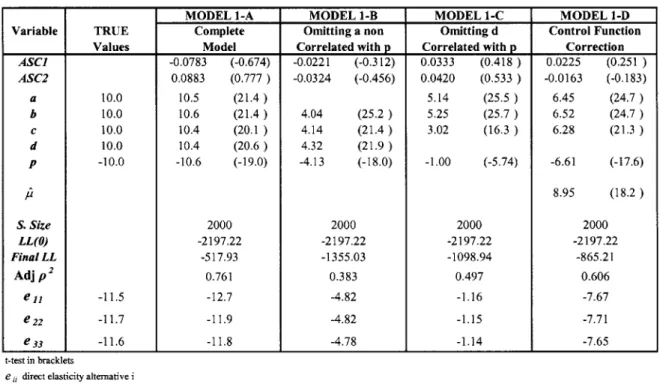
Table 4-1 Monte Carlo Experiment One. Models 1-A to 1-D ... 56

Table 4-2 Price Equation Model 1 -D and 1-E ... 58

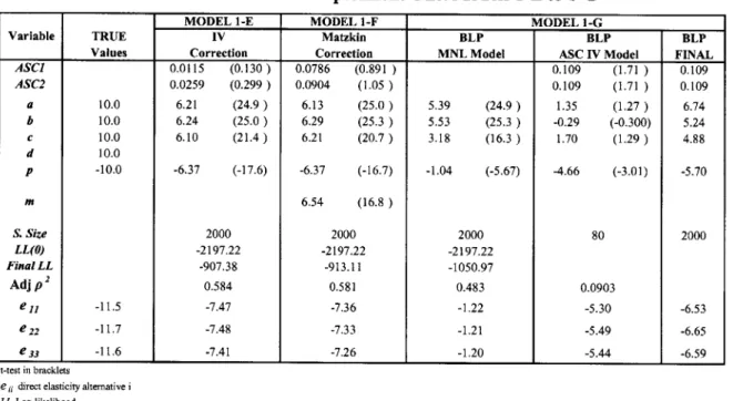
Table 4-3 Monte Carlo Experiment One. Models 1 -E to 1 -G ... 62

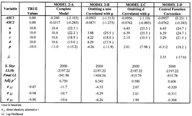
Table 4-4 Monte Carlo Experiment Two. Models 2-A to 2-D ... 63

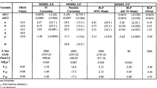
Table 4-5 Monte Carlo Experiment Two. Models 2-E to 2-G... 64

Table 4-6 Price Equation Model 2-D and 2-E ... 64

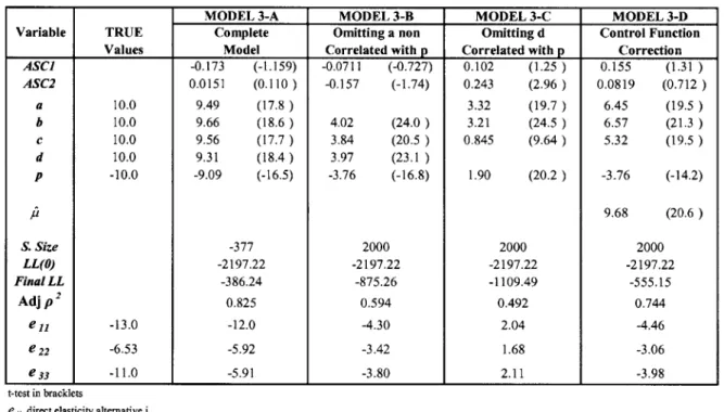
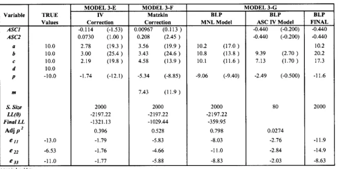
Table 4-7 Monte Carlo Experiment Three. Models 3-A to 3-D ... 65

Table 4-8 Monte Carlo Experiment Three. Models 3-E to 3-G...66

Table 4-9 Price Equation Model 3-D and 3-E ... 67

Table 4-10 Monte Carlo Experiment Four. Models 4-A to 4-D ... 68

Table 4-11 Monte Carlo Experiment Four. Models 4-E to 4-G... 68

Table 4-12 Price Equation Model 4-D and 4-E ... 69

Table 4-13 Non Parametric Corrections for Control-Function... 70

Table 5-1 Price Equation Instrumental Variables OLS ... 82

List of Figures

Figure 1-1 Urban System Modeling Framework... 9

Figure 1-2: Example of an Omitted Quality Attribute... 11

Figure 3-1 Identification of Simultaneous Equations ... 36

Figure 5-1 Study Area EOD 2001 Santiago de Chile: Municipalities and Sectors ... 74

Chapter 1

Introduction

1.1 Motivation

The development of models to understand the behavior of an urban system as a whole is crucial, not only for the evaluation and exploration of policies to manage the level of pollution and congestion in the cities, but also for solving problems such as the efficient

provision of: utilities, transportation infrastructure and schools.

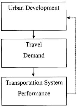
A general framework to model the decisions relevant to travel demand and their

interactions with the urban system can be stated in three interrelated stages, corresponding to the urban development or land-use, the travel demand and the

transportation system performance (Figure 1-1). Depending on the level of detail and the

scale of the analysis, this framework can be used to model aggregated flows of trips by geographical zones or disaggregated household and individual decisions that lead to a demand for travel, including mobility and lifestyle, activity/travel scheduling, and their revisions (Ben-Akiva et al., 1996).

Urban Development

Travel

Demand

Transportation System

Performance

Figure 1-1 Urban System Modeling Framework

The key task in capturing the long-term behavior of an urban system is to forecast the changes in land-use patterns. Thus, understanding the behavior of the land market is crucial in the development of policy tools for shaping the urban system or managing the externalities associated with it. This observation is particularly relevant for cities of developing countries, such as Mexico or Chile, where dramatic changes in density and income composition of suburban areas is expected due to the simultaneous increase of motorization, income and highway infrastructure, just as it was observed in United States cities after World War II (Weisbord et al., 1980).

The land market itself is a very complex system comprised of many subsystems. There is an industrial and a residential land market. Each market has unique dynamics resulting from the interaction between agents offering and demanding industrial land or dwelling units. This research only focuses on the residential market due to its primary effect on the urban system through the determination of the core part of the origin-destination trip matrix. Furthermore, for the sake of simplicity, it will be assumed that the supply of dwelling units is exogenous, and thus, this thesis will be focused on residential location choice models.

1.2 Statement of the Problem

Within this framework, an econometric issue of relevance arises. Consider a situation where households choose to buy or rent dwelling units of a specific type in certain locations. If this problem is modeled using an aggregated framework, the number of dwelling units sold will necessarily depend upon the price and other characteristics of the dwelling unit. At the same time, the price of the dwelling unit will depend upon the demand for the dwelling unit. The simultaneous determination of these variables causes the independent variables of the model to be correlated with the error term (non-orthogonality), breaking then a crucial assumption made in the estimation of the model, which makes the estimated parameters inconsistent and biased.

Even in a discrete choice framework, where the simultaneous determination effect can be argued not to occur, a different but very plausible problem can arise. If a quality attribute, that is relevant for the decision maker, is not observed by the researcher and it is correlated with the price of the dwelling unit, the price will be correlated with the error term causing, again, a non-orthogonality problem.

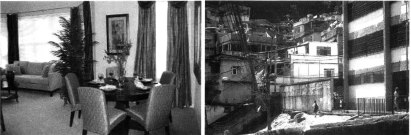
Consider for example the residential location choice decision problem described in Figure 1-2. In this case, the decision maker can perceive all the attributes of the alternatives in her choice set, including the non-measurable one that is explained through the photographs. However the researcher can observe only the number of bedrooms, the size, the price and whether utilities are provided or not for each alternative. In the viewpoint of the researcher, individuals who decide to live in apartment A would be not

very smart because they reject such a bargain as B or, more formally, just not sensitive to

price.

However, what it is really occurring is that a relevant quality attribute, which is correlated with the price, has being omitted. It will be shown in this thesis that this problem implies that an upward bias for the price parameter (a negative parameter that becomes more positive) will usually occur in residential location models.

A) 1 Bedroom; 70 m2; with utilities; $2000 B) 1 Bedroom; 70 m2; with utilities; $100

Figure 1-2: Example of an Omitted Quality Attribute

Many empirical residential location choice models (Bhat and Guo, 2004; Sermons and Koppelman, 2001; Levine, 1998; Waddell, 1992, 1996; Quigley 1976) have reported non-significant, small or even positive dwelling unit price parameters. The hypothesis of this thesis is that this is caused by endogeneity due to the existence of some omitted attributes that are correlated with the dwelling unit's price. This hypothesis has been considered only in very few studies related to residential location (Bayer et al., 2004 and Ferreira, 2004). Furthermore, endogeneity in discrete choice models is an area of current development in econometrics, which makes the study of its effects in residential location modeling a challenging and interesting issue to address.

1.3 Thesis Objectives and Outline

The objectives of this thesis are the following:

1. To develop a conceptual framework for the treatment of endogeneity in

residential location choice models.

2. To test the available methods to address endogeneity in discrete choice models of residential location, using a set of Monte Carlo experiments.

3. To verify the relevance of the endogeneity problem and the quality of the

proposed correction methods, by estimating a model of residential location based on real data.

The structure of this thesis is as follows. The next chapter presents a critical analysis of the state of the art in residential location modeling in light of the problem of price endogeneity. The third chapter analyzes different issues related to the treatment of endogeneity in discrete choice models of residential location. In Chapter 4, a comparison of the different available methods to address endogeneity in discrete choice models of residential location is made through a set of Monte Carlo experiments. The fifth chapter is an application of the most suitable method to address endogeneity in residential location, as found in Chapter 4, to real data from Santiago de Chile. Finally, Chapter 6 presents the general conclusions and recommendations for further research.

Chapter 2

Residential Location Modeling

This chapter reviews the state of the art in residential location modeling in light of the price endogeneity problem. This task is accomplished in four steps. First, the chapter reviews theoretical considerations in modeling the residential location market. Second, the chapter reviews specification issues of relevance in the development of residential location choice models, including the selection of explanatory variables, sample and choice set definition, the level of aggregation of the alternatives and econometric issues related to the error structure that can be expected in modeling this market. Afterwards, a brief discussion about the relationship between land-use and transportation is presented. Finally a set of recent residential location models where price endogeneity appears to be

2.1 Theoretical Considerations in Modeling the

Residential Location Market

2.1.1 Microeconomic Framework

The general microeconomic framework to model residential location is based on the assumption that each household as a whole maximizes the combined utility of its members. This utility depends on the time and goods associated with the activities that each household's member performs, including transportation, work and other derived activities. It is also assumed that, conditional on a specific location i, households face constraints associated with: the available time that their members have to perform the activities, their budgets and the feasibility of developing each set of activities and their associated goods consumption.

The solution of this problem, conditional on each residential location i, corresponds to the set of activities that each member of each household perform and the associated time assignments and goods consumption. If these optimal values are replaced in the objective function of the utility maximization problem, it will be obtained what is known as the

conditional indirect utility function.

Finally, it is assumed that households choose the residential location that has the larger conditional indirect utility function plus a random component, in what is known as the Random Utility Model (Ben-Akiva and Lerman, 1985).

2.1.2 Optimality of Current Location

The basic assumption required for modeling residential location choice using a utility maximization framework is that households are located in places that maximize their utilities given their budgets and other constraints. However, in reality, many households are located in non-optimal places due to the diverse costs (pecuniary, social or even emotional) associated with moving.

One way of addressing this problem is to model first the decision of whether to move, in order to consider the effect of inertia in the model. One example of this approach is Weisbord et al. (1980) where the authors used a Nested Logit model. However, to build a model like that, detailed information about the previous locations of the households is required, data that are not usually available, or at least, not with the required detail.

Another way to model the decision to move by any household is to add to the utility of alternatives new locations an additional cost associated with moving that is calculated based on external data and assumptions. However, the difficulty in obtaining adequate data to apply that approach makes its application infeasible.

Finally, other issue that would be relevant in addressing household residential location optimality is to consider a model to predict when a specific household decides to change from the rental to the ownership market, because each ownership status carries very different moving costs.

2.1.3 Market Size

Within this setting, the size of the market (that is, the number of households that want to move and the dwelling units that are available) will be a function of the characteristics of the system and also a function of time. This is because, even considering that the supply of new dwelling units is exogenous, any change in the characteristics of the system would affect the perception held by specific households about their present residential location, relative to the other alternatives. Sometimes, the effects of these changes will be strong enough to make the households to decide moving and thus to enter into the group of households seeking residential locations (the demand) and, at the same time, add their current dwelling units into the group of offered ones (the supply).

These changes can be external to the household, such as the provision of new transportation infrastructure or changes in school quality, crime or pollution rates in specific areas; or internal to the household such as changes in income, the births of children or problems with the neighbors.

2.1.4 Dwelling Unit's Price

Modeling dwelling unit's price in residential market is a challenging task because it does not only depend upon dwelling unit's attributes but also upon the differences between the demand and the supply which are caused both by the difficulties in adjusting the supply to the demand in the short run and because each good in this market has almost unique characteristics. Examples of different approaches to this problem can be found in Martinez and Henriquez (2005), Bayer et al. (2004) and Waddell (1996).

Martinez and Henriquez (2005) proposed a theoretically derived expression for the endogenous determination of dwelling unit's price or rent. This expression (2-1) is the expected value of the highest bid offered by the households for a specific dwelling unit and is derived under the assumption that bids are random variables that depend upon dwelling unit's characteristics. In their model, the bids consist of a systematic component

B and an error term that is assumed to be identically and independently distributed (iid)

Extreme Value (0, p). Additionally, y is Euler's constant, ri is the price of a dwelling unit of type v located in i and Ng is the number of households of type g.

(2-1) r, = 1 In I Ng exp(pBg +

Conversely, Bayer et al. (2004) considered that dwelling unit's prices are endogenously determined as the prices that clear the market in an iterative process. This means that prices are adjusted up to the point where each dwelling unit is assigned to exactly one household. The authors affirm, based on the study of Berry (1994), that this procedure has a unique solution for the prices.

In reality, is not necessary that the each dwelling unit becomes chosen or that all households are able to find an affordable housing solution in the equilibrium. However, modeling a situation like that requires detailed information about the stock availability and household's budget, which is not usually available.

Finally, Waddell (1996) and Waddell and Borning (2004) in their URBANSIM model, used a micro-simulation approach to forecast the behavior of the land market. This model is implemented as a set of interacting model components that represent the

major actors and choices in the urban system. Within this framework, the author considered a hedonic price model that simulates the land prices for each modeling zone (cell), output that is used as an input by other model components. No theoretical considerations for the equilibrium in the system are stated by the authors.

2.1.5 Dwelling Unit's Supply

To model the long term equilibrium of the residential location market is necessary to have a model of dwelling units supply. This is because real estate developers should respond to price variations in the market, building more dwelling units where they expect to get greater benefits, changing with their decisions the system equilibrium by pulling down the higher dwelling units' prices and then affecting the demand structure in the whole system.

In this sense, the model of Martinez and Henriquez (2005) represents an interesting theoretical framework where real estates dwelling unit's supply are treated as random variables under a profit maximization framework that is consistent with the dwelling unit's demand model. On the other hand, the URBANSIM model of Waddell and

Borning (2004) offers an attractive micro-simulation approach for this problem.

2.1.6 Workplace and Residential Location

A final question to address in modeling the equilibrium of the residential location

market is the relationship between workplace location and residential location decisions. It can be argued that the choice of work location is made conditional on the residential location, or visa versa. Alternatively, it can be argued that residential location decision is made in a longer time frame and thus, what households consider in their decision of where to live is the probability of having access to good jobs in each specific location.

If workplace determines residential location, the model must consider the distance

is to consider a more elaborated measure of the generalized cost, such as the expected maximum utility of the available modes, which depends on travel time and costs.

If, on the contrary, the residential location determines the workplace location, the

residential location model should include a work accessibility measure, instead of the actual distance to workplace. Even though, if in this case the distance to workplace is included instead of the accessibility, this variable should be significant anyway, because actual work location can be seen as a proxy for work accessibility, because it is more probable to find a job in places where more jobs are offered. However, the meaning of the estimated parameters in that case will not be clear.

Now, if it is assumed that workplace location determines residential location and that residential location determines workplace location simultaneously, it would be necessary to address an endogeneity problem arising from this simultaneous determination, equivalent to the one described in this thesis for price in residential location modeling. The study of this effect is left for further research.

Finally, if residential location and workplace location occur in different time frames, what should be included in the model is the accessibility to a variety of workplaces instead of the actual distance to workplace.

2.2

Model Specification Issues

In this section is presented a set of specification issues that have to be considered in residential location modeling. These issues are related to the definition of the sample, the level of aggregation of the alternatives, the definition of the choice set, the error specification, and the type of explanatory variables that should be considered in residential location modeling.

2.2.1 Sample Definition

One alternative proposed in the literature to achieve the requirement of considering only optimally located households in the sample, is to include in the sample only households that have moved recently because it can be argued that these are the only ones that, for sure, are located in an optimum place (Weisbord et al., 1980). Another way of achieving this objective could be to consider only renters in the sample, under the assumption that they have lower moving cots associated. Against both the recently-moved and the renter assumptions can be argued that the modeling sample in these cases will not be representative of the whole population and that the selection criteria would imply such a reduction in the sample size that other estimation issues can arise.

Other issue to address in the sample definition is about the possibility that not every household chooses its location optimally on the basis of the attributes of the dwelling units. This is especially relevant in developing countries, where very-low income households live where they live because this dwelling unit is provided for free, or at a very non-market low price, by a relative (in what is known as "Allegados" or "Arrimados") or, in some cases, the place where they live was the result of the collective appropriation of a portion of land by the force (what is known as a "Toma" or "Ocupas"). In both cases, it is arguable that the households will be indeed located at their optimal locations but, because they do not have real feasible alternatives to their actual location, they cannot be modeled under the utility maximization framework used in this thesis.

Beyond this, if it would be possible to conduct a data collection activity specific for this research, without having to rely only on existing mobility surveys or census data, the ideal procedure would be to survey households that have recently changed their location. The survey would include questions about the alternatives that were considered in the process of choosing a residential location and their attributes.

2.2.2 Level of Aggregation of the Alternatives

A key consideration in modeling residential location choice is the definition of the

alternatives. The usual approach is to consider administrative zones as the source to measure the spatial factors and as the alternatives themselves. This method follows Lerman (1975) who, arguing that the data is usually not available at an individual level, proposed a Multinomial Logit (MNL) choice model (2-2) where alternatives are groups of housing units instead of individual units. Within this framework, the author considered also a size variable (Ben-Akiva and Lerman, 1985) to account for the aggregation of

alternatives.

Two problems arise with the aggregated approach described above. The first is that the definition of the neighborhood or the area of influence of the shared attributes is left as purely exogenous and subject to administrative definitions that are not necessarily aligned with the research interests. The second problem is that, by aggregating, the rich variability that can be found among dwelling units in the aggregated areas is lost.

An alternative approach consists in considering each dwelling unit as an alternative, recovering the neighborhood information on administrative zones (as in Bayer et al. 2004) or using some kind of Geographic Information System (GIS) to recover neighborhood information searching for the average attributes within some general or specific dwelling unit area. Working on this idea, Guo (2004) found that neighborhood socioeconomic attributes are important in a small contiguous area of the dwelling unit and land-use attributes are relevant in a larger radius.

2.2.3 Choice Set definition

The definition of the choice set in residential location modeling is not trivial because the huge number of alternatives to consider (potentially, each dwelling unit in the city) creates a computational burden of considerable proportions. The usual approach to deal with this problem is to use a randomly chosen sample of the available alternatives. McFadden (1978) proved that the estimated parameters using this procedure are consistent for a MNL model. The problem with the use of the MNL model in residential location modeling is that it can usually be rejected because, for example, nearby areas share unobserved attributes that make them correlated.

Another approach is to consider only a reduced set of feasible alternatives, where each available alternative can be selected using an ordered availability assumption (Ben-Akiva and Boccara, 1995). In the case of residential location modeling, this means that the probability that each alternative belongs to the choice set is determined as a function of the difference between some socio-demographic characteristic of the household at their current location and those of each considered alternative. The idea behind this is that alternatives that are too different to the current location are not really considered by the households when deciding where to move.

Finally, about which dwelling units to consider as available in the choice set, an additional argument in favor of considering only households that have recently changed their location is that, if it is considered a model where each dwelling unit is an alternative, it can be argued that the only available dwelling units correspond precisely to the ones that have been chosen by a household recently. The other dwelling units that should be considered as being available in the model are the ones that are unoccupied. However, this last piece of information is usually difficult to collect.

2.2.4 Error Specification

The assumptions that are made on the error structure of the discrete choice model imply a trade-off between tractability and accuracy. The simplest assumption to make is to accept that utility errors are iid Extreme Value (0,p), which leads to a very

attractive closed form (Ben-Akiva and Lerman, 1985) for the choice probability in what is known as the Multinomial Logit (MNL) model

[22

P

eui

(2-2) P,(i)= Pr Vj" + <" > Max. " +.

j

I i - jECn

where P,(i) is the probability that individual n chooses alternative i, Vi" is the deterministic part of the utility Uj" that individual n retrieves from alternative i and C, is the set of alternatives available to individual n. The parameter p is the scale parameter of the Extreme Value distribution, which is inversely proportional to the standard deviation

of the error and has to be normalized, usually to one, because it is non-identifiable.

The basic problem with the MNL model is that it is not able to reproduce the non-uniform substitution rates that can be expected between alternatives. This problem can be expressed in what is known as the Independence from Irrelevant Alternatives (IIA) property. For model (2-2), the ratio of the probabilities of two alternatives is independent of all other alternatives.

This means that, for example, if a person chooses between hotels for vacation, and the five-stars hotels double their previous prices, the change in the probabilities of all other types of hotels (including the half-star ones) will be the same, instead of, as it is intuitively expected, have a stronger effect in the ones with better rating. It has to be noted however that, the IIA property no longer holds in aggregated predictions for heterogeneous population, reducing its impact.

Many ways of avoiding the IIA property have been proposed in the literature. First, this can be solved by considering that the errors are Multivariate Normal, which leads to the Probit model, where the correlation matrix is not forced to be diagonal. The problem however is that the Probit model does not have a closed form and requires numerical integration, which increases the computational burden, making the problem almost intractable (even for today's computers) for a model with over six alternatives.

One closed form model that belongs to the Generalized Extreme Value (GEV) models and allows for correlation between groups of alternatives is the Nested Logit (NL) model (Ben-Akiva and Lerman, 1985). In this model, correlated alternatives are grouped in

nests allowing different scale factors for each group. The probability that an individual n chooses a specific alternative i will depend on the product of the probability of choosing the nest k, where i belongs, and the probability of choosing the alternative conditional on the nest being chosen.

The expression for this probability is (2-3), where p and A are scale parameters of the errors of the root and the nest respectively. These parameters are not jointly identifiable, problem that can be solved by fixing one of them, usually p, to be equal to one.

(2-3) P

(i)

(k)P (i/k)=

expV, _{I expA"Vj"}

leNests(n) IECnVA

The utility of each nest is calculated as the Expected Maximum Utility (EMU) or inclusive value of the alternatives contained in the nest.

(2-4) V = in exp(2 Vj +

One problem that makes this model unsuitable for residential location choice is the fact that it is restricted to have each alternative in only one nest. This is a problem because correlation should exist between each pair of adjacent zones or areas and not in separated groups. This means that what is required is to have each zone belonging to a different nest with each of its adjacent zones.

A variation of the NL model that allows for such correlation is the Cross Nested Logit

model (Vovsha, 1997) where each alternative is allowed to belong to more than one nest considering a specific weight for each one.

Other method proposed in the literature to deal with the 1IA property is the Logit Kernel or Mixed Logit model (Train, 2003). This method in addition to the Extreme Value error of the MNL model also includes other error that introduces correlation among the alternatives. The choice probabilities are obtained by numerical or Monte Carlo integration.

This model can take into account, for example, the specification of flexible disturbances or random parameters. For example, if the subset of alternatives S are correlated, then it would be possible to specify an additional error e with distributionf(e)

in the utility of the alternatives that belong to S and calculate P,(i) , the probability that an individual n chooses alternative i , as in (2-5),where 4s is a dummy that is equal to one if

i belongs to S and zero otherwise. The most efficient way found so far to calculate this

integral numerically is the Halton Draws procedure (Train, 2000).

(25 exp (V. _{+ 8se)}

(2-5) P(0.)=

f(e)de

f Iexp V" + se

jeA(n)

An example where the error specification issues in residential location modeling are considered through closed forms and flexible error structures is the work of Bhat and Guo (2004). The authors developed a model that they called a Mixed Spatially Correlated Logit (MSCL) model for location choices, that is basically a Cross Nested Logit where each zone belongs to a different nest with each of its adjacent zones and, additionally, some parameters of the model are considered random in the estimation using the Logit Kernel approach.

The motivation of the authors behind this approach is to add some flexibility to the disturbances terms of the RUM without increasing too much the dimension of the integration problem in the Logit Kernel problem. This is done by representing all this interaction using only one estimable parameter that captures the correlation effect between contiguous spatial units.

The authors applied their model to a case study with 236 observations, comparing a

MNL model versus their MSCL model. Despite the fact that some improvements are

observed, it can't be asserted from the paper if these improvements came from the fact that some parameters in the MSCL model were considered random and/or because of the inclusion of the spatial correction effect.

Moreover, the central motivation in developing the MSCL, that is, to have a computationally cheaper alternative to Logit Kernel to address zonal correlation, was not tested, so no conclusions can be obtained about its real advantages.

2.2.5

Relevant Attributes and Characteristics in Residential

Location Choice Decision

In this section, a general review of the type of location attributes and household characteristics that have been found in the literature to be relevant in residential location choice is presented.

The relevant attributes in residential location choice models can be divided in two classes, the ones that belong to the specific dwelling unit and others related to the

environment (neighborhood) where it is located. The effect of each of these variables will depend on the socio-economic characteristics of the household involved. The results reported in the literature for these parameters so far are diverse and sometimes

contradictory or against intuition (Guo, 2004).

Examples of attributes that belong to the specific dwelling unit are the commuting time associated with this specific dwelling unit, its price, size, age, number of rooms, architectural style, and if it is a single house, a duplex, a condominium or an apartment.

All these attributes, but the price, share the feature of been completely exogenous to the

residential location process.

The attributes related to the environment (neighborhood) where the dwelling unit is located can also be divided in two classes. The first class of neighborhood attributes is formed by socio-racial-economic attributes such as, for example, race and ethnicity, income, education, average age and family status. These neighborhood attributes are grouped in a different class because it has been empirically found that households tend to cluster themselves in groups that share similar attributes. Thus, they are expected to enter the utility function as the difference between household value for the correspondent characteristics and neighborhood attribute average.

Explanations for this phenomenon go in the line of easiness for establishing social networks, the type of educational experiences that children can have as the result of their interaction with the neighbors (Bayer, et al, 2004), segregation in the real estate market (especially by racial origin) or self characteristics validation. These neighborhood attributes share also the feature of being endogenous to the residential location process.

This means that they are, at the same time, the result of the residential location process and a variable considered in the choice model.

The second class of attributes related to dwelling unit's environment corresponds to the ones that are not valued in terms of their difference with household characteristics. Examples of these types of attributes are accessibility and attractiveness, residential

density, school quality, safety, street cleanliness or land-uses expressed as the percentage of parks, industrial or trash dump areas. All these neighborhood attributes, except perhaps the residential density, share also the feature of been exogenous, unless a very long-term analysis is considered.

Finally, household characteristics are not only relevant in the location choice process in terms of their difference with neighborhood attributes. It is also important to consider the differences in the perception of the attributes that different household type or members should have. For example, it can be expected that low-income households perceive housing price as more important than high-income households. It have also been found that women tend to have more sensitivity to commuting time relative to males what have been explained as a result of the dual role of women who have to be near enough home to take care of children and other households tasks (Sermons and Koppelman 2001). Also, it can be expected for example that families with children would have a greater preference for houses instead of apartments. Thus, it would be necessary to consider in modeling residential location parameters differentiated by household socio-economic characteristics such as the ones described here.

2.3 Land Use and Transportation

2.3.1 About the Magnitude of the Link between Land-use and

Transportation

Pickrell (1999) show that between 1900 and 1960, the densities of new residential developments in a sample of 10 United States (US) large urban areas, have been constantly declining up to be one fifth of the original ones. This can be argued to be the effect of the development of transportation technologies in the form of private automobile, motorbus, transit and highways, together with the rise in family income.

However, the author claims that nowadays the impact of transportation on land-use in

US cities should be considerably less important. This is because the marginal effect of

new transportation improvements should be smaller due to the characteristics of the technological development curve and because new transportation investments would probably be more or less redundant to already existing ones, reducing then their net impact.

Other fact that reduces the flexibility in residential location nowadays is the grater share of multi-workers households, which makes a residential move substantially more difficult.

In the case of developing countries such a Mexico or Chile, it can be expected that the phenomenon observed in US cities in the first half of the twentieth century, that is, a simultaneous increase in income, motorization and a substantial increase in highway infrastructure, would have the mid-term effect of increasing the sprawl of the city, moving higher income households to the lower density suburbs. However, the second argument about the multi-workers household composition is equally valid for developing countries' cities so, it can be expected that the net effect would be lower than the effect in the US.

Pickrell (1999) also discusses the feasibility of developing a computational model to forecast the long term behavior of the entire system of land-use and transportation. The author states that experience have shown that the great amount of information needed and

the simplifying assumptions used in the current models have made them of little accuracy or robustness in the prediction of the behavior of the system so far.

2.3.2 Measuring the Relationship between Land-use and

Transportation

When deciding where to live, households as a whole have to make a trade-off between dwelling unit's amenities and travel cost to actual and potential activities

developed by each of its' members.

Because individuals has more than one transportation mode alternative to reach their destinations is necessary to consider, for each origin and destination, the EMU that the individual can obtain by using any of the available modes, defined as the Generalized Cost (GC). The GC that household n that is located at I perceives by traveling to place J has a nice closed form (2-6) if it is assumed that the error terms of the utility function are

iid Extreme Value (0,A) (Ben-Akiva and Lerman, 1985), where Vk''" is the utility of mode k that is available to travel from Ito J for household n.

(2-6) GCn(I, J)= IIn exp(Z Vk''" +

In the same way, in the case where accessibility (ACC) to different activities is what matters, this value can be calculated as the EMU of visiting, from location I, each and every location J to develop a specific activity, expression that again has a closed form

(2-7) if it is assumed that errors are iid Extreme Value (0,u).

(2-7) ACCn(I)= In vexp(pv'''" +

-JeDest

)

Martinez (1995) used the same approach to also define the concept of attractiveness (ATT), which is the expected maximum utility of being visited from other locations as follows, if the errors are assumed to be iid Extreme Value (0,r/).

(2-8) A TT(J)= 1In Iexp(V'''" +L

More elaborated expressions for measures of the relationship between transportation and land-use can be drawn by considering all the omitted attributes and perceptions of the households by latent variables (Walker, 2001). However, this approach requires more data and has not yet been applied to build satisfactorily models of residential choice.

2.4 Price Endogeneity in Econometric Models of

Residential Location

In order to show the potential relevance of the issues addressed in this thesis, in this section is reviewed as set of studies in residential location where price endogeneity appears to be a relevant issue that was not considered. Afterwards are presented a residential location model where price endogeneity was treated but possibly ineffectively and one case where almost the same considerations taken into account in this thesis were used.

One work where endogeneity appears to be an issue and was not treated' is Sermons and Koppelman (2001). In this work, the authors modeled couples commute behavior in residential location and found a small (but significant) housing cost parameter, which could be the result of the price endogeneity problem studied in this thesis.

Another source of endogeneity in this model could be simultaneous determination of the work location of each member of the modeled couple, what could cause the commuting distance parameters to be inconsistently estimated. In this case, it would be useful to apply some variation of the methods developed by Blundell and Powel (2004) to correct for male-female working salary endogeneity.

Housing price was not significant in the model developed by Bhat and Guo (2004). They also found that school quality was not significant in the residential location process of single worker households, attributing the unintuitive result to the lack of detail in how the urban attributes were measured. A similar result is found by Waddell (1996) for single worker households and by Quigley (1976) and Levine (1998) for high income households. Waddell (1992) also found a positive, but small, elasticity of price for white workers.

It is highly unlikely that these results represent real behavioral characteristics of single workers, high income or white households. The real problem behind these findings should be either data problems or the price endogeneity bias analyzed in this thesis.

Unsuccessful attempts were done to obtain the databases used in the cited studies, and thus, it was not possible to test these hypotheses directly.

For the best of the knowledge of the author of this thesis only two works have considered the treatment of price endogeneity in discrete choice models or residential location. The first one is Bayer et al. (2004). In their research about racial segregation in the housing market, the authors did correct for price endogeneity using the method proposed by Berry, Levinsohn and Pakes (BLP, 1995), which is explained latter in this thesis. The author found considerably more negative parameters for the dwelling unit's price when comparing their model to a non-corrected one.

However, the big problem with this study is that the authors considered one alternative specific constant for each and every household, which implies that the estimated parameters are inconsistent due to the incidental parameters problem (Wooldridge, 2002). The problem is that, as the sample size increases, the size of each "market" stays fix (in one) making impossible to estimate their fix-effect parameter consistently. Furthermore, the inconsistent estimation of the fix-effect parameter contaminates the estimation of the other parameters in the model, which makes all estimated parameters inconsistent.

The other example where price endogeneity is treated in residential location modeling is Ferreira (2004), who was a research assistant in the Bayer et al.(2004) study. The author analyzed taxes incentives in residential location market. In his model the author considered a correction for price endogeneity based in the control-function method proposed by Petrin and Train (2004). The only argument against the procedure applied is that in this case the author used, as instruments for the price, the attributes of nearby dwelling units (following the idea of Bresnaham,1997) instead of the prices of nearby dwelling units themselves, as proposed by Hausman (1997), which will be claimed to be a better approach in section 3.1.3. The author found considerably more negative price parameters when the endogeneity correction was applied.

Chapter 3

Endogeneity in Econometric Models

The objective of this chapter is to describe all the relevant issues in understanding the causes, consequences, and treatment of endogeneity in econometric models in light of residential location modeling.

With this purpose, will be first presented a review of what is endogeneity, when it is likely to occur, and how it can be solved in the case of linear econometric models. Using this as a background, are then analyzed in detail the available methods to treat endogeneity in discrete choice models. Finally a review of relevant applications of these methods in the literature is presented and discussed.

3.1 Endogeneity in Linear Models

3.1.1 When Endogeneity is Likely to Occur in Linear Models

Consider the linear regression model (3-1), where Y is a vector defined as the dependent variable to be explained by the independent variables contained in the matrix

X, 8 is a vector of parameters, and e is a vector of errors or values that makes

expression (3-1) an identity.

(3-1) Y = X8 +

The estimator of the vector of parameters / that minimizes the square of the modeling error (Greene, 2003), which is commonly identified as the ordinary least

squares (OLS) estimator, is expression (3-2).

(3-2) Minfl .6 = Minfg(Y -X)(Y-X) ->p=(XTXY XTY

A desired small sample property for the estimator 6 is to be unbiased. This means that, at least on average, 8 should be equal to the true parameter ,6 or, formally, that its expected value, conditional on X, should be equal to

fi.

E(6X)= (XTX X E Y/X =(XTX (Xg+ E[e/XD

(3-3) _{=f6+ (X X)}1 _XTE1e/X]

BIAS

Thus, a necessary condition for 8 to be unbiased is to have e independent of X or, equivalently, the expectation of e given X equals zero (E[e/X] = 0). Having

E[E/X] # 0 is commonly called non-orthogonality and, for the purpose of this thesis, it

Omitted Attributes

One example of when endogeneity occurs is the case when the researcher omits an attribute that is relevant in the true model. To demonstrate this, assume that in the true model an additional variable U is relevant, so that the model can be expressed as shown in (3-4).

(3-4) Y = X/+Ua+,6;E(e/XU)=0; [XU]fullrank.

Now, assume that the matrix of variables U is unobserved by the researcher but that the true model is still (3-4). Then, if the expectation of the OLS estimator of the parameter

#

E(//X) = (XTX

X

(Xf

(3-5) = (XTX) [XTX + XTUa]

= '8 +(X XY XTUa

BIAS

Hence, /OLs will be unbiased if and only if the observed variables X are orthogonal

with the unobserved ones U or, if the vector of parameters a is zero. Otherwise, /3oLs

will be upward biased if X and U are positively (negatively) correlated, and a is positive (negative) and downward biased otherwise.

Errors in Variables

Another example of when endogeneity can occur is the case when the independent variables are measured with error. Consider the true model (3-6), where a single variable

Xt* determines the dependent variable yt, and where, instead of xt* , xt is observed, which

is a noisy version of xt* as is shown in (3-7).

(3-6) y, = a + x, *+ ,, E

[e

(3-7) x, = x,*+2

(3-7) yt = -+ X t 2t

In this case, as is shown in expression (3-8), the independent variable x, will be correlated with c2t because of (3-7) and then with the error term e, as long as 62,1 is

different from zero, that is, if errors in variables exist and 8 is different from zero. If this

problem exists, IlOLS will be biased toward zero in what is known as the "attenuation

bias" or the "iron law of econometrics" (Greene, 2003).

Simultaneous Determination

Another example where the non-orthogonality problem arises is the case where the dependent and at least one of the independent variables are simultaneously or endogenously determined through different equations. This case can commonly occur in a model of market equilibrium between demand and supply where the selling price pt determines the quantity produced qt in the supply equation and the quantity produced determines the price in the demand equation, which depends also on another variable I, as is shown in expression (3-9).

Supply q, = 81 p, + s1,

Demand p, =/8 ₂₁q, + 822

1

+ 62t

The fact that the dependent variable is correlated with the error term, both in the supply and the demand equations, follows directly from an argument equivalent to the problem of errors in variables shown in (3-6)-(3-8) if one equation is replaced on the

other, taking the dependent variable of each one as the true one.

As in the errors in variables case, if each equation of model (3-9) is estimated independently, a bias towards zero will occur. Instead, if the simultaneity is taken into account for both equations, it will be possible to estimate the parameter of the price in the supply equation consistently, but not to identify the parameters of the demand one.

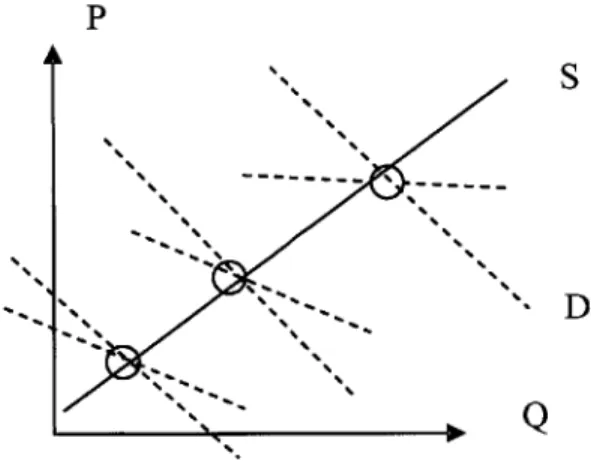
To understand why the identification and consistency results described above occur, recall first that what can be observed are equilibrium points of the price and the quantity traded in the market (Figure 3-1). In the case described in (3-9) the supply equation is

invariant and the different equilibrium points are explained by a set of demand curves that is not unique because of variations of I.

P

..

\

S

D

Figure 3-1 Identification of Simultaneous Equations

Then, the demand equation remained unidentified but, at the same time, its variation

justified

This identification result can be shown through the derivation of the reduced

form

q, = alI, +, =J - 19192i, + A 2 t 11 t supply

(3-10)

-lll

p, = a21it + 1, _ - 22 it + P21 61t + c2t Demand

1--pns 1$

Thus, if equations (3-10) are estimated by OLS, the parameter of the supply equation in (3 -9) can be identified as8

pI

/asl

parameter

#21

3.1.2 Instrumental Variables, the Method to Treat Endogeneity

in Linear Models

The method to address the problem of non-orthogonality or endogeneity in linear models is called the instrumental variables (IV) procedure (Greene, 2003). It corresponds to project the dependent variable that is correlated with the error term onto a space that is orthogonal to the error's space, which is defined by another variable called instrument. Then, the estimated (instrumented) dependent variable will not suffer the non-orthogonality problem and can be used to estimate the model consistently.

Consider again the model (3-1) where the endogeneity problem exists. Consider also a matrix of variables Z with rank(Z)= L > rank(X)= K; and a matrix

(TxK) =Z(TxL)A(LxK) where A is a function of the data X. Thus, the following estimator ofp8 can be defined.

(3-11) ), = (W Xy WTY

The conditions under which the estimator (3-11) is unbiased are analyzed in (3-12).

E[,iv /X] = E(WTX WTY/X]= ELwX W(Xg + E)/X

(3-12) =8 + (W TXY E[WTe/X] = ,q+(WT X E[(Z) e/X]

- 8 + (Tz~"x)1 ~T[T

BIAS

Thus, in order to have an unbiased2 _{estimator of 8 using (3-11) it would be required}

that Z were, at the same time, orthogonal to the error term EIZ T] = 0 and correlated with

X E[ZTX] 0.

It can be shown that the value of A that minimizes the variance of 8,, corresponds

to A = V-Z TX, where V is some consistent estimator of the variance of Z T.. In the case

where e is spherical, that is var(e) = U2I, the estimator of the inverse of the variance

2 To have an equivalent consistency result for large sample, the following weaker conditions are needed: