Great tits and the city: Distribution of genomic diversity and gene-environment associations along an urbanization gradient

HAL Id: hal-02367249

https://hal.archives-ouvertes.fr/hal-02367249

Submitted on 17 Nov 2019

HAL is a multi-disciplinary open access

archive for the deposit and dissemination of

sci-entific research documents, whether they are

pub-lished or not. The documents may come from

teaching and research institutions in France or

abroad, or from public or private research centers.

L’archive ouverte pluridisciplinaire HAL, est

destinée au dépôt et à la diffusion de documents

scientifiques de niveau recherche, publiés ou non,

émanant des établissements d’enseignement et de

recherche français ou étrangers, des laboratoires

publics ou privés.

diversity and gene-environment associations along an

urbanization gradient

Charles Perrier, Ana Lozano del Campo, Marta Szulkin, Virginie Demeyrier,

Arnaud Grégoire, Anne Charmantier

To cite this version:

Charles Perrier, Ana Lozano del Campo, Marta Szulkin, Virginie Demeyrier, Arnaud Grégoire, et

al.. Great tits and the city: Distribution of genomic diversity and gene-environment associations

along an urbanization gradient. Evolutionary Applications, Blackwell, 2018, 11 (5), pp.593-613.

�10.1111/eva.12580�. �hal-02367249�

Evolutionary Applications. 2017;1–21. wileyonlinelibrary.com/journal/eva  

|

  1 Received: 30 May 2017 

|

  Accepted: 19 November 2017

DOI: 10.1111/eva.12580 O R I G I N A L A R T I C L E

Great tits and the city: Distribution of genomic diversity and

gene–environment associations along an urbanization gradient

Charles Perrier

1

_{| Ana Lozano del Campo}

1

_{| Marta Szulkin}

1,2

_|

Virginie Demeyrier

1

_{| Arnaud Gregoire}

1

_{| Anne Charmantier}

1

This is an open access article under the terms of the Creative Commons Attribution License, which permits use, distribution and reproduction in any medium, provided the original work is properly cited. © 2017 The Authors. Evolutionary Applications published by John Wiley & Sons Ltd 1_{Centre d’Ecologie Fonctionnelle et Evolutive,} CEFE UMR 5175, Campus CNRS, Université de Montpellier, Montpellier Cedex 5, France 2_{Wild Urban Evolution and} Ecology Laboratory, Centre of New Technologies, University of Warsaw, Warsaw, Poland Correspondence Charles Perrier, Centre d’Ecologie Fonctionnelle et Evolutive, CEFE UMR 5175, Campus CNRS, Université de Montpellier, Montpellier Cedex 5, France. Email: charles5perrier@gmail.com Funding information European Research Council, Grant/Award Number: ERC-2013-StG-337365-SHE; OSU-OREME

Abstract

Urbanization is a growing concern challenging the evolutionary potential of wild popu-lations by reducing genetic diversity and imposing new selection regimes affecting many key fitness traits. However, genomic footprints of urbanization have received little attention so far. Using RAD sequencing, we investigated the genomewide effects of urbanization on neutral and adaptive genomic diversity in 140 adult great tits Parus major collected in locations with contrasted urbanization levels (from a natural forest to highly urbanized areas of a city; Montpellier, France). Heterozygosity was slightly lower in the more urbanized sites compared to the more rural ones. Low but significant effect of urbanization on genetic differentiation was found, at the site level but not at the nest level, indicative of the geographic scale of urbanization impact and of the potential for local adaptation despite gene flow. Gene–environment association tests identified numerous SNPs with small association scores to urbanization, distributed across the genome, from which a subset of 97 SNPs explained up to 81% of the vari-ance in urbanization, overall suggesting a polygenic response to selection in the urban environment. These findings open stimulating perspectives for broader applications of high- resolution genomic tools on other cities and larger sample sizes to investigate the consistency of the effects of urbanization on the spatial distribution of genetic diver-sity and the polygenic nature of gene–urbanization association. K E Y W O R D S genomic, great tit, selection, SNP, urbanization

1 | INTRODUCTION

Humans substantially modify natural ecosystems, especially since the industrial revolution (Vitousek, Mooney, Lubchenco, & Melillo, 1997). Urbanization, the process by which cities are formed and expand, is one of the major threats to natural ecosystems. Urbanization affects habitats, notably resulting in their loss, modification, or fragmentation (Crooks & Sanjayan, 2006). Urbanization also results in chemical, noise, and light pollution, altered temperatures, novel epidemics, predation risks, all in all resulting in the modification of species assemblage and demography (Aronson et al., 2014; Galbraith, Jones, Beggs, Parry, & Stanley, 2017; Shryock, Marzluff, & Moskal, 2017; Vincze et al., 2017), phenotypic traits (Alberti et al., 2017; Biard et al., 2017; Suárez- Rodríguez, Montero- Montoya, & Macías Garcia, 2017), and evolution-ary dynamics (Alberti, 2015; Anderies, Katti, & Shochat, 2007; Hendry, Gotanda, & Svensson, 2017). Although urbanization generally results in dramatic local biodiversity declines as a lot of species avoid or are unsuccessful in urban environments, other species are able to cope

and even take advantage of such environmental change via plastic or adaptive responses (Lancaster & Rees, 1979; Møller et al., 2012). Understanding the demographic, ecological, and evolutionary pro-cesses resulting from urbanization is thus becoming an important goal in conservation and evolutionary biology (Donihue & Lambert, 2014).

Urbanization has various impacts on the demography of species, affecting the density of individuals, their dispersal, their survival, and their reproductive rates, and ultimately affecting genetic diversity and differentiation among populations. In particular, fragmentation and degradation of habitats strongly affect dispersal of individuals and population sizes. Because it leads to reduced dispersal and gene flow, fragmentation caused by urbanization can result in lower genetic diversity and higher neutral genetic differentiation among populations (Gortat et al., 2015; Lourenço, Álvarez, Wang, & Velo- Antón, 2017; Munshi- South, Zolnik, & Harris, 2016) as well as increased relatedness among individuals (Chiappero et al., 2011). The impact of these effects of fragmentation on demography and genetic differentiation will, how-ever, depend on the dispersal capacity of species. While fragmentation can enhance genetic differentiation in rodents and amphibians as they are susceptible to terrestrial barriers (Gortat, Rutkowski, Gryczynska- Siemiatkowska, Kozakiewicz, & Kozakiewicz, 2012; Lourenço et al., 2017), bird species will generally be less affected as they can fly be-tween suitable habitats (Partecke, Gwinner, & Bensch, 2006; but see Björklund, Ruiz, & Senar, 2010). The decrease in habitat quality caused by urbanization may also result in reduced genetic diversity and in-creased differentiation if population size decreases, thereby increasing the amount of genetic drift (Munshi- South et al., 2016). Nevertheless, if fragmentation does not impede dispersal, asymmetrical gene flow can occur from more productive populations inhabiting natural habi-tats into less productive ones inhabiting unfavorable habitats, that is, highly urbanized areas (Björklund et al., 2010). Lastly, habitat choice could also reinforce a neutral genetic differentiation between pop-ulations inhabiting natural and urbanized environments. Although habitat choice is known to influence patterns of dispersal, gene flow, genetic differentiation, and evolutionary processes (Dreiss et al., 2012; Edelaar & Bolnick, 2012), it has received limited attention in the case of urbanization studies. If it imposes divergent selection pressures compared to those act-ing in wild environments, urbanization may also result in divergence at particular loci underlying adaptive evolution in urbanized environ-ments, detectable through genomic approaches. Many studies have recently investigated genomic footprints of divergent selection that may be implicated in local adaptations, in a wide range of species and contexts (Savolainen, Lascoux, & Merilä, 2013; Tigano & Friesen, 2016). However, these studies were largely restricted to wild popu-lations in natural environments (e.g., well- known examples in stick-lebacks (Gasterosteus aculeatus; Hohenlohe et al., 2010), in Atlantic cod (Gadus morhua; Nielsen et al., 2009), or in lizards (Lacerta lepida; Nunes, Beaumont, Butlin, & Paulo, 2010)). Only a small number of studies have focused on urban genomics, investigating footprints of divergent selection between natural and urbanized environments based on genomewide data. Harris, Munshi- South, Obergfell, and O’Neill (2012) and Harris and Munshi- South (2017) investigated

genomic shifts in white- footed mice Peromyscus leucopus in New York City, and examined the evolutionary consequences of urbanization. Among the thousands of SNPs screened using genome scans, they identified several candidate genes possibly under positive selection in urban versus rural populations of P. leucopus. These outliers were notably involved in metabolic functions and were potentially underly-ing rapid local adaptation in urbanizing habitats where P. leucopus may use different food resources. Such pioneering urban genomic studies have begun to pave the road for investigating genomic footprints of divergent selection between natural and urban wild populations. With the rapid spread of new generation sequencing tools, similar genome-wide studies like the one of Harris and Munshi- South (2017) can be applied to nonmodel organisms, in search of novel candidate genes potentially under selection.

The great tit (Parus major) is a small passerine species that has be-come a model study organism in behavioral ecology and evolutionary biology. Great tits are widespread and abundant across Eurasia and can be found in a wide variety of environments, from natural forests to highly urbanized cities. Previous studies based on microsatellite loci showed relatively small genetic differentiation across Europe, yet higher differentiation among southern populations (Lemoine et al., 2016) as well as within the city of Barcelona (Björklund et al., 2010). Studies comparing the life history and physiology of great tits in forest versus city habitats have recently revealed that, compared to their forest conspecifics, urban great tits lay earlier and smaller clutches, they display faster breath rates and faster exploration scores in a novel environment, have higher levels of neophilia, and their off-spring fledge in poorer condition (Bailly et al., 2016; Charmantier, Demeyrier, Lambrechts, Perret, & Gregoire, 2017; Marzluff, 2001; Sprau, Mouchet, & Dingemanse, 2016; Torné- Noguera, Pagani- Núñez, & Senar, 2014; Tryjanowski et al., 2016). Given this strong phenotypic divergence and as genomic resources have recently been developed for this species (Laine et al., 2016), the great tit is a good candidate species for urban genomic studies investigating both neutral genetic differentiation between urban and natural populations and potential genomic bases underlying adaptations to urban environments. Here, we took advantage of the recent advances in RAD sequenc-ing techniques (restriction site- associated DNA sequencing; see Etter, Bassham, Hohenlohe, Johnson, & Cresko, 2011 and Rowe, Renaut, & Guggisberg, 2011 for introductions about RAD sequencing) and of the availability of the great tit genome to perform a genomewide analysis of individuals breeding across a gradient of urbanization, looking for effects of urbanization on both neutral and adaptive genetic differen-tiation. Specifically, the first aim of this study was to test the impact of the local level of urbanization on the extent of genomewide genetic diversity and structure in urban great tits. Although small genetic dif- ferentiation was expected given recent empirical findings in this spe-cies (Laine et al., 2016; Lemoine et al., 2016), we hypothesized that significant population structure and reduction in diversity may occur among populations found in areas with different levels of urbaniza-tion (Björklund et al., 2010), potentially resulting from the interplay between reduced dispersal and population size, habitat choice, and local adaptation. The second aim was to search for genomic footprints

of divergent selection between sites with different levels of urbaniza-tion, and gene–urbanization associations, that may be implicated in adaptation to urban life (Harris et al., 2012).

2 | METHODS

2.1 | Study sites, sampling

A total of 140 great tits were sampled from 87 nest boxes posi-tioned in five sites with different levels of urbanization in the city of Montpellier (France) and in a rural site: the deciduous forest of La Rouvière (Montarnaud, France) where great tits have been moni-tored since 1991 (Table 1, Figure 1a). The total number of monitored nest boxes available for great tits was 180 in the city and 70 in the Rouvière forest. The city of Montpellier experienced a high human population expansion since the middle of the 19th century to early 21st century, growing from around 35,000 to 280,000 inhabitants. Six sites are equipped with monitored nest boxes: the zoo of Lunaret (ZOO) which includes a large forested area; Grammont (GRA), Mas Nouguier (MNO), Font- Colombe (FCO) and Mosson (MOS) which all contain a mixture of urbanized sectors and parks; and La Rouvière (ROU) which is an oak forest located 20 km northwest of Montpellier (Table 1, Figure 1). Great tit breeding was monitored in all nest boxes from April to July each year since 1991 in La Rouvière forest and since 2011 in the city of Montpellier. Parents were caught in nest boxes when their nest-lings were 10 days old. In 2014, 5–30 μl of blood was sampled from adult breeders for later DNA extraction. Blood was taken from a small neck vein or from a wing vein and stored at 4°C in Queen’s buffer (Seutin, White, & Boag, 1991).

2.2 | Urbanization level

From April to May 2012, vegetation cover (surface covered by oaks, trees and green spaces), and light (artificial night lighting), air and noise (using car traffic to reflect as a proxy) pollutions were recorded within a 50- m- radius disk around each nest box (see Demeyrier, Lambrechts, Perret, and Gregoire (2016) for details) which corresponds to the main area prospected by the focal pair within a breeding season (Perrins, 1979). A principal component analysis (PCA) of these variables re-vealed that they were highly correlated (Demeyrier et al., 2016). Therefore, the first axis of the PCA was chosen as a single continuous variable to reflect the urbanization level at each nest box (Table 1 and Figure 1a), which was thereafter referred to as nest- level urbaniza- tion. Differences in nest- level urbanization among sites were inves-tigated using an ANOVA and a Tukey’s HSD test in R (R Core Team,

T A B L E   1   Site name, abbreviation, average nest coordinate per site, average nest urbanization level (see methods), sample size (before and

after removing highly related individuals), and observed heterozygosity (Ho). Sites were ordered by average urbanization level. For urbanization level and observed heterozygosity, letters indicate significant differences

Site Abbreviation Coordinates (lat. long.) Urbanization level Sample size Ho

Mas- Nouguier MNO 43.586 3.862 +2.32a _{18/18 0.285}a

Font- Colombe FCO 43.597 3.834 +0.87b _{10/10 0.290}abc

Mosson MOS 43.637 3.812 +0.70b _{5/5 0.290}abc

Grammont GRA 43.617 3.932 −0.31c _{29/26 0.289}ab Rouvière ROU 43.664 3.668 −1.94d _{47/41 0.294}c Zoo ZOO 43.642 3.878 −2.19d _{31/25 0.292}bc F I G U R E   1   (a) Map of the sampled sites with color scaled urbanization. (b) Boxplots of urbanization scores per site. Correspondences of site abbreviations are found in Table 1 a b b _c d _d Longitud e —2 —1 01 2 43.70 _(a) 43.65 43.60 ROU MOS FCO ZOO CITY MNO GRA (b) Urbanization 2 1 0 −1 −2 43.55 3.6 3.7 3.9 4.0 Longitude

2016). Additionally, latitude and longitude were recorded at each nest box (Table 1) with a GPS (Garmin© GSPmap® _62s).

2.3 | DNA extraction and RAD sequencing

DNA extraction was performed using Qiagen DNeasy Blood & Tissue kits. DNA extraction was randomized across sites. DNA was quan-tified using a NanoDrop ND8000 spectrophotometer and then a Qubit 2.0 fluorometer with the DNA HS assay kit (Life Technologies). DNA quality was checked on agarose gels. DNA extracts (including two replicates in different lanes to estimate the consistency of the analyses) were sent to MGX (CNRS, Montpellier) for libraries prepara-tion using restriction site- associated DNA sequencing (RAD seq; Baird et al., 2008) with the enzyme SbfI. Each individual was identified using a unique 6- nucleotide tag. Individual samples were multiplexed in equimolar proportions by groups of 29 or 30 individuals. Individuals were randomized across groups. Each group was sequenced on one of seven lanes of an Illumina HiSeq 2000 (on these lanes were also in-cluded juvenile great tit individuals from the same sites but that were not used in this study).

2.4 | SNP calling and filtering

Raw sequences were inspected with FastQC (Andrews, 2010) for qual- ity controls. Reads were treated with Cutadapt (Martin, 2011) to re-move potential fragments of Illumina adapters. A 10% mismatch was allowed in the adapter sequence. Stacks 1.32 (Catchen, Hohenlohe, Bassham, Amores, & Cresko, 2013) was used to demultiplex reads, identify RAD loci, and call single nucleotide polymorphisms (SNPs). Reads were filtered for overall quality, demultiplexed, and trimmed to 85 bp using process_radtags. One mismatch in the barcode sequence was allowed. BWA- MEM 0.7.13 (Li & Durbin, 2009) was used to map individual sequences against the reference genome of the Great tit (Laine et al., 2016) using default options. The total assembled con-tigs spans 1.0 Gb, for an estimated genome size of 1.2 Gb. We used samtools 0.1.19 to build and sort bam files (Li et al., 2009). We used

pstacks, with a minimum stack depth of 5 (m = 5), the SNP model, and

α = .05. cstacks was used to build the catalogue of loci using n = 3. With sstacks, loci were searched against the catalog of loci. Finally, individuals were genotyped using the stacks’s populations module and filtered using VCFtools (Danecek et al., 2011). Loci were retained if genotyped in at least 90% of individuals (all individuals from all sites grouped) with individual minimal read depth of 8 (“na” replaced geno-types below a read depth of 8), with a minimum average read depth of 20 across all genotypes, a maximum average read depth of 100 across all genotypes, and a minor allele frequency above 5% (MAF ≥ 0.05) across all individuals (all individuals from all sites grouped). We veri-fied that each individual was genotyped for at least 95% of all loci. We filtered the entire dataset for deviations from Hardy–Weinberg equilibrium at the SNP level (HWE, p- value ≥ .01) in ROU. We did not filter specifically the other populations for HWE due to smaller sam-ple sizes, and we considered that most of the significant deviations in every site would also be found in ROU given the high gene flow among the populations. This HWE filtering step was mainly applied to remove sequencing or SNP calling errors as well as paralogous se-quences (Waples, 2015). In turn, this should not interfere with the detection of divergent selection between urban and forest popula-tions as HWE is estimated locally but not across sites. We investigated the average decay of LD in chromosomes 1–20 (the chromosomes on which most of the SNPs (86%) were found), in ZOO (as LD was very similar in all populations), using gdsfmt and SNPRelate (Zheng et al., 2012). Although the data are not phased, this coarse estimate of LD was useful to evaluate the physical distance between outlier SNPs and neighboring genes that may be relevant for our functional analysis and to discuss the proportion of the genome covered by our RADseq analysis. Finally, we calculated identity- by- state IBS among individuals using the R packages gdsfmt and SNPRelate to (i) estimate consistency of SNP calling on the two replicated individuals, and (ii) identify highly related individuals. One individual was removed for each pair of highly related individuals (i.e., siblings and parent–offspring) to produce a dataset called “no-family-ties.” The rationale for this procedure is that related individuals could artificially increase Fst between groups of in-dividuals (see also Szulkin, Gagnaire, Bierne, & Charmantier, 2016).

2.5 | Investigation of genetic diversity,

relatedness, and differentiation

Genetic diversity was inferred through individual observed het-erozygosity (Ho) on the no-family-ties dataset. Ho was estimated using VCFtools. Differences in individual Ho were investigated using ANOVAs in R, with individuals grouped in the six sites. Finer compari-sons of Ho between pairs of sites were achieved using a Tukey’s HSD test in R. Population structure was investigated via identity- by- state (IBS), fix-ation index (Fst), a principal component analysis (PCA), and a discriminant principal component analysis (DAPC). We calculated IBS among indi-viduals of the entire dataset to determine whether relatedness among individuals differed between sites and to test whether we could infer dispersal events (via the presence of highly related individuals found in different sites). Differences in IBS between sites were assessed in R using an ANOVA (see also Szulkin et al. (2016) for more details on the method). Fst were estimated between the six sites using GenoDive (Meirmans & van Tienderen, 2004), which takes into account Weir and Cockerham’s optimizations of Wright’s theoretical index (Wright, 1951) to control for unequal sample sizes (Weir & Cockerham, 1984). The sig-nificance of pairwise Fst values was tested through 1,000 permutations in GenoDive. We estimated the Fst using both the entire dataset and the no-family-ties dataset. We also estimated a global Fst (Weir & Cockerham, 1984) between sites for each SNP using SNPRelate and represented with a Manhattan plot. The most likely number of genetic cluster was estimated using the function find.clusters from the R package adegenet (Jombart, 2008) on the no-family-ties dataset. We used a principal com-ponent analysis (PCA) using the function snpgdsPCA implemented in the R package SNPRelate to depict genetic structure among the sites, using both the entire dataset and the no-family-ties dataset. Finally, we used a discriminant analysis of principal components (DAPC) implemented

in the R package adegenet to depict genetic structure among the sites, using the no-family-ties dataset. We used the cross- validation procedure from the adegenet package using the function xvalDapc, to identify the optimal number of principal components, reassigning 30% of the individ-uals, with a training set based on 70% of the individuals and replicating 100 times the procedure for each set of PCs from 10 to 45 by steps of 5, and then from 5 to 15 by steps of 1.

2.6 | Effect of geographic

distance and of urbanization on genetic diversity, sites

differentiation and individual relatedness

First, we estimated the correlations between urbanization and ob-served heterozygosity, at the site level and at the nest level. Second, to infer the effect of geographic distance and of urbanization difference on dispersal and genetic differentiation, we inferred correla-tions between (i) Fst (estimated on the no-family-ties dataset) and geo-graphic distance, (ii) Fst and urbanization difference, (iii) IBS (estimated on entire dataset) and geographic distance, and (iv) IBS and urbanization dif-ference. The correlations of either Fst or IBS with geographic distance are used to infer potential isolation by distance, whereby dispersal and ac-cumulation of genetic differentiation increase with geographic distance between populations. The correlations of either Fst or IBS with urbaniza- tion difference are used to infer potential habitat choice, whereby dis-persal and accumulation of genetic differentiation increase with habitat differences. Fst is more likely to capture long- term accumulation of allele frequency differences while IBS captures the present time distribution of relatedness and therefore the dispersal events.

Third, to investigate simultaneously the influence of latitude, longitude, and urbanization on the genetic distance among individu-als (using the entire dataset), we used a redundancy analysis (RDA), which is a constrained version of PCA (Legendre & Fortin, 2010; Legendre & Legendre, 2012), implemented in the Vegan R package (Oksanen et al., 2007). Using this RDA, we first investigated the por- tion of the genetic variability that could be explained by a constrain-ing covariance matrix consisting of latitude, longitude, and nest- level urbanization for each individual. We tested the global significance following 1,000 permutations. Then, we ran marginal effects permu-tation tests to address the significance of each variable. Ultimately, we focused on the effect of nest- level urbanization alone, using partial RDA first taking into account the effect of latitude and longi-tude. Significance was tested running 1,000 permutations. Because the indirect effect of nest- level urbanization on genetic structure could operate at a scale larger than the 50- m- radius sphere around the nests, we performed a second RDA using a site- specific average level of urbanization (calculated for each site as the average of the nest- level urbanization values) rather than a nest- level urbanization.

2.7 | Search for SNPs, genes, and Gene Ontologies

associated with urbanization

We used latent factor mixed model (LFMM; Frichot, Schoville, Bouchard, & Francois, 2013) on the entire dataset to identify SNPs

potentially under divergent selection along the urbanization gradi-ent. As urbanization may act as a selection force at different spatial scale on great tits, we implemented three tests using fine- to large- scale incorporation of urbanization. We first used the fine- scale nest- level urbanization values (50 m radius from their nest) as explanatory variable (referred as test A). In test B, we used site- specific average urbanization. In test C, we used a binary test comparing ROU (coded as 0) and the city sites (coded as 1). These three tests were performed again, excluding the ZOO (re-ferred as tests D, E, F). This was motivated by the fact that birds in the Zoo may experience similar selection pressures as ROU birds (as similar low urbanization values were observed), while being in the pe-rimeter of the city. Therefore, gene flow among urbanized sites from the city and the zoo could limit the response to locally forestlike envi-ronment in the zoo and limit the power of outlier tests. Moreover, this site also represented an opportunity to avoid circularity, first identify-ing outlier loci excluding ZOO and subsequently inspecting by mean of PCAs (detailed next paragraph) whether ZOO individuals were closer to urban or forest birds. ZOO individuals closer to urban birds would suggest restricted effect of selection relatively to gene flow, at small spatial scale, or absence of habitat choice influenced by outlier loci. In contrast, ZOO individuals closer to forest birds would suggest rela- tively important response to selection at small spatial scale, or of hab-itat choice influenced by outlier loci.

Five runs (10,000 burn- in, 100,000 iterations) per LFMM test were used to obtain average z- scores, representing the strength of the association between a SNP and an explanatory variable, and associ-ated p- values, assuming a unique genetic cluster. We displayed the Z- scores with Manhattan plots. We estimated q- values from LFMM’s

p- values, for each of the six tests separately, using the R package fdrtool (Strimmer, 2008) and reported the distribution of the results

across the six tests (A–F) using (i) Manhattan plots for each test, (ii) histograms of outliers’ z- score distributions for each test, (iii) biplots between tests, and (iv) Venn diagrams (R package VennDiagram, Chen & Boutros, 2011; and the Web- based tool InteractiVenn, Heberle, Meirelles, da Silva, Telles, & Minghim, 2015). On each Manhattan plot was superposed a line representing a kernel- smoothing moving aver- age using a 10- Mb- long window sliding by steps of 10 Kb, to deter-mine whether outlier SNPs were found in genomic areas with average high association with urbanization. We reported a table of the SNPs found in the top 10 of each test, to provide more functional details on the putative genes in which these outliers were found. We performed PCAs, using the function snpgdsPCA implemented in the R package SNPRelate, followed by linear models in R, to inves-tigate the proportion of variance in individuals’ scores of urbanization at the nest and at the site explained by the genetic distances between individuals when considering several outlier lists of SNPs with q- values <.05, as well as the entire set of SNPs. This procedure was achieved to inspect the power of gene–urbanization associations. Either the PC1 or PC2 or both were considered to explain individual nest- or site- level urbanization, using a linear model in R. The PCA, realized with the list obtained from tests D, E, and F, was furthermore used to visually inspect the genetic distance of ZOO with other sites.

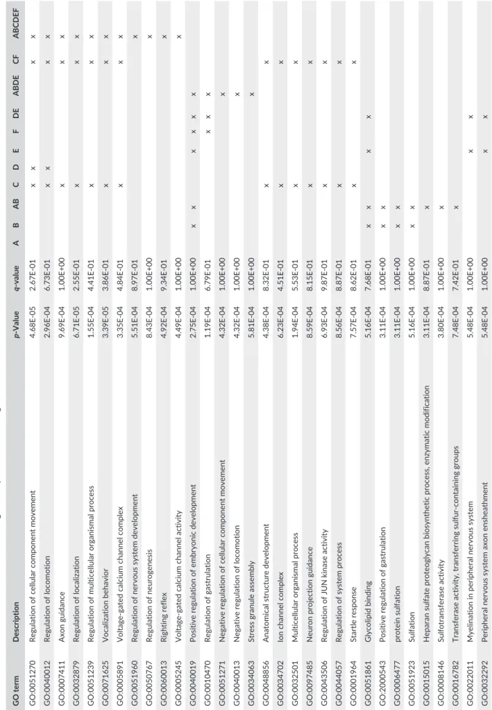
To assess to which extent genomic associations with urbanizations were polygenic, we inferred, using linear models, the proportion of variance in nest- level urbanization that was explained by PCAs using an increasing number of SNPs, from 1 to 49,969, sorted by decreasing Z- score in test A. Although this is a circular examination, it is primarily an attempt to investigate the cumulative nature of the top outlier SNPs from gene–urbanization association tests. We considered only PC1 as this axis captured most of the variation in urbanization while analyzing outliers from test A (as it will be explained in the result section). Genes were extracted from the great tit reference annotation (NCBI Parus major Annotation Release 100). We reported the genes found in the aforementioned lists. Then, gene ontology (GO) enrichment tests, which aim to identify potentially enriched GO terms, were performed in GOrilla (Eden, Navon, Steinfeld, Lipson, & Yakhini, 2009), using as background list of genes the entire set of genes found among the SNPs used in this study (n = 5,276). We tested for GO enrichment among genes founds for several lists of outliers (each test separately and several combinations of tests). Enrichment tests were corrected with the FDR method.

3 | RESULTS

3.1 | Environmental data

Average urbanization level per site ranged from −2.19 in ZOO to 2.32 in MNO (Table 1, Figure 1a,b). The maximum nest- level urbanization was 2.9 in MNO, and the minimum was −2.7 in ZOO. The fact that ZOO was found less urbanized than ROU (the forest) is in part due to the absence of motorized vehicles in the zoo, unlike in the forest, as well as its huge vegetation cover. Nest- level urbanization was sig-nificantly different across sites (ANOVA, F = 180.3, p- value < 2e- 16). Tukey’s HSD test revealed that all pairs of sites had significantly dif-ferent means in nest- level urbanization scores (p < .05), except FCO and MOS (p = .99) and ZOO and ROU (p = .52).

3.2 | SNP calling

Sequencing RAD tags for 140 breeding great tits resulted in a total of 1,815,823,241 raw sequences, with an average of 7,793,233 reads per individual. 107,413 loci were identified in the stacks cata-log. After filtering for depth coverage, HWE, and MAF, 49,969 SNPs in 32,756 loci were kept in the final dataset, roughly one locus every 37 Kb. The missing rate per individual ranged from 0.001 to 0.058, with a median of 0.024. The missing rate per locus ranged from 0.000 to 0.100, with a median of 0.014. The average read depth across genotypes (SNP * Individual) was 72 (Appendix S1), and the fifth percentile was 24. Average linkage disequilibrium decreased rapidly within the first Kb between SNPs and then continued to decrease slowly (Appendix S2). The IBSs between each replicated samples were high, respectively, of 0.9999 and 0.9987. Replicates were removed from all subsequent analyses. To construct the no-family-ties dataset, twelve individuals with IBS superior to 0.80 with other individuals were removed (three in GRA, six in ZOO, and six in ROU).

3.3 | Genetic diversity, relatedness, and

differentiation

There was a general pattern of reduced diversity in individuals from the four most urbanized city sites, in particular MNO, com-pared to ZOO and to ROU. The observed genomewide observed heterozygosity (Ho) was different among sites (ANOVA: F = 11.6,

p- value = .000866, Table 1). Ho was lower in MNO (the most

ur-banized site) than in ROU and in ZOO. Ho was lower in GRA than in ROU.

Pairwise IBS between individuals ranged from 0.73 to 0.89 and was in average of 0.75 (Figure 2a,b). Average IBS values were not significantly different between the sites, using either the entire data-set (ANOVA: F = 1.99, p- value = .08) or the no-family-ties- datasignificantly different between the sites, using either the entire data-set (ANOVA: F = 1.62, p- value = .15).

The Fst ranged from 0.004 to 0.009, for an average of 0.007 (Table 2). Fsts were significant for all of the comparisons. The Fst between the most and least urbanized site was 0.008. When highly related individuals were kept, the genomewide differentiation among the sites ranged from 0.004 to 0.013 for an average of 0.009, illustrating that keeping these individuals could have slightly biased the results. Although average Fst was very low, there were several SNPs showing relatively high Fst (Appendix S3a). The find.clusters analysis supported the existence of only one genetic cluster. The cross- validation procedure identified n = 10 as the optimal number of principal components of allelic variation to retain for the DAPC (Appendix S4a,b). This use of 10 principal components in the DAPC resulted in average in 82% (median = 87%) of correct individual as-signments to their population, revealing a moderate discrimination power of the six groups (Appendix S4b) clearly rejecting the pan-mixia hypothesis. The DAPC (Appendix S4d) based on 10 principal components and the PCA (Figure 4a–d) both depicted a clear ge- netic structure between the sites but no particular pattern of differ-entiation in link with urbanization. The PCA performed better when the no- family- tie dataset containing no highly related individuals was used (Figure 3c,d) than when they were included (Figure 3a,b).

3.4 | Effect of geographic distance and urbanization

on genetic diversity and differentiation

At the site level, observed heterozygosity was significantly cor-related with urbanization (r2 _{= .76, p- value = .02; Figure 4). At the}

individual level, observed heterozygosity was also significantly cor-related with urbanization but explained much less variation (r2 _{= .09,} p- value = .0003). Genetic differentiation between sites tended (no significant cor-relation) to increase with geographic distance and with urbanization difference (Figure 5a,b). All, except one, of the few high IBS indices (superior or equal to 0.80, probably corresponding to parent–offspring, full- sib, or half- sib relationships) were found within sites, at small geo-graphic distances (Figure 5c). The rest of the IBS indices (below 0.80) only slightly decreased with geographic distance and urbanization dif-ference (Figure 5c,d).

When genetic variance among genotypes was constrained by the full RDA model for latitude, longitude, and nest- level urbanization, the proportion of variance explained was significant globally (p < .001, Table 3), although only the single effect of longitude (p < .001) was sig-nificant, while nest- level urbanization and latitude had nonsignificant effects (p = .16 and .17, respectively). Using the partial RDA model to test for a nest- level urbanization effect, after subtracting the effect of longitude and latitude, the proportion of variance explained was not significant (p = .21). Urbanization at the nest explained 0.75% of the total genotypic variance (p = .20). When genetic variance among genotypes was constrained by the full RDA model for latitude, longitude, and average urbanization at the site rather than at the nest, the proportion of variance explained was significant globally (p < .001, Table 3), and both longitude and average urbanization at the site had significant effects (p < .001 and p = .01, respectively). After subtracting the effect of longitude and latitude, the proportion of variance explained using the partial RDA model was still significant (p = .02). Urbanization average per site explained 0.78% of the total genotypic variance (p = .01).

3.5 | SNPs and genes associated with

urbanization and gene ontology enrichment

Several SNPs exhibited relatively high scores of association with ur- banization (Figure 6). These association scores were on average de-coupled from average Fst between sites (Appendix S3b,c). Although F I G U R E   2   (a) Heatmap of genomic relatedness (IBS) among individuals. (b) Boxplots of IBS among individuals in the six sites. Site abbreviations correspond to Table 1 0.75 0.80 0.85 IBS

MNO FCO MOS GRA ZOO ROU

MNO FCO MOS GRA ZOO ROU

0.75 0.80 0.85 IB S (a) (b) T A B L E   2   Fst (upper triangle) and associated p- values (lower triangle) among locations, estimated using the dataset with/without highly related individuals

MNO FCO MOS GRA ROU ZOO

MNO 0.004/0.004 0.009/0.009 0.009/0.008 0.009/0.008 0.012/0.008 FCO 0.001/0.001 0.006/0.006 0.009/0.007 0.007/0.006 0.011/0.006 MOS 0.001/0.001 0.001/0.001 0.010/0.009 0.007/0.006 0.012/0.008 GRA 0.001/0.001 0.001/0.001 0.009/0.001 0.009/0.007 0.012/0.007 ROU 0.001/0.001 0.002/0.001 0.012/0.019 0.001/0.001 0.013/0.008 ZOO 0.001/0.001 0.003/0.001 0.012/0.030 0.001/0.001 0.001/0.001

several hundred outliers were identified, there was little evidence for large z- score peaks that could have been synonymous of strong as-sociation at a particular genomic region (but see, e.g., the outlier SNPs in the middle of chromosome 3, Figure 6). The correlations were high between the z- scores obtained with the quantitative tests at the nest level and at the site level with or without ZOO (r2 _{= .79 between A and} B, r2 _{= .79 between D and E, p < .001, Appendix S5). The correlations} were also relatively high between similar tests made with or without the ZOO (r2 _{AD = .59; r}2 _{BE > .58; r}2 _{CF = .75, p < .001). In turn, the}

correlations were relatively small between z- scores values obtained for the quantitative tests (A, B, D and E) and for the binary tests (C and F; average r2 _{= .28, ranging from 0.08 to 0.48, p < .001, Appendix S5).} At a q- value threshold of 0.05, 45, 89, 514, 81, 114, and 224, SNPs were significant for each of the six tests A, B, C, D, E, and F, respec-tively (Appendix S6), for a total of 667 SNPs when the six lists were merged. Similar type of tests (quantitative vs. binary) had relatively large proportions of shared outlier SNPs compared to dissimilar tests (Appendix S7). Seven outlier SNPs were found, at q- values <.05 for all of the tests (Appendix S7e). 415 outlier SNPs were only found in one of the six tests. As expected, the PCAs using outlier SNPs revealed patterns of genetic structure linked to urbanization (Figure 7), in contrast with the PCA using the entire SNP dataset that showed very little genetic structure linked to urbanization (Figure 3b and d) but rather a geo-graphic structure (Figure 3a and c). The first axis of the PCA based on the entire set of SNPs explained 3% of the variation in urbanization score at the nest (Table 4). Taken together, the first and second axes of this PCA explained 6% of the variation in urbanization score at the nest. Similar results were obtained for the site- level urbaniza-tion scores, the first axis of the PCA explained 4% of the variation and 8% were explained by both axes together. In turn, 81% of vari-ance in site- level urbanization was explained by the first axis of the PCA summarizing interindividual genomic variation at 97 SNPs with

q- values <.05 for gene–urbanization tests A & B grouped (Table 4,

Figure 7a,b). In contrast, only 15% of variance in urbanization was explained by the first axis of the PCA summarizing interindividual genomic variation at the top 514 SNPs with q- values <.05 for gene– urbanization test C (Table 4, Figure 7e,f), rather depicting ROU ver-sus city differentiation, as expected from the nature of the test C

F I G U R E   3   Principal component analyses of individual genotypes based on (a and b) the entire dataset of 49,969 SNPs and all of the 140 individuals, (c and d), the entire dataset of SNPs and no-family-ties dataset. In (a and c), color code refers to populations. In (b and d), color code refers to urbanization level o o ooo _o o o o o o o o o oo o o o o oo oo o o o oooo o o o o o o o ooo oo o o o_oo o o ooooo_oo o o oooooo_o o o ooo o ooo o oo o o o o o o oo_o o o o_ooo o o o o o oo o oo o oooo oo o oo_oo ooo o o o o o o o o o o oooo_o o o ooo oo 0.0 0.1 0.2 0.3 0.4 −0.2 0.0 0.2 0.4 Eigenvector 1 (2.0%) Eigenvector 2 (1.5%) o o o o o o FCO GRA MNO MOS ROU ZOO o o ooo _o o o o o o o o o oo o o o o oo oo o o o oooo o o o o o o o ooo oo o o o_oo o o ooooo_oo o o oooooo_o o o ooo o ooo o oo o o o o o o oo oo o o_ooo o o o o o oo o oo o oooo oo o oo_oo ooo o o o o o o o o o o o o o_o o o o ooo o o 0.0 0.1 0.2 0.3 0.4 −0.2 0.0 0.2 0.4 Eigenvector 1 (2.0%) Eigenvector 2 (1.5%) o o o o o o_o o o o o o o o o o o o o _o o oo o o o o o o o o o o o o oo o o o o o o o o o o o o o o o o o o o o o _o o o o o o o o o o_o o o o o o o o o o o o o o o o o o o o _ooo o o o o o_o o o o o o o oo _o o o o o o o o o o o o o o −0.05 0.00 0.05 −0.1 5− 0.05 0.05 0.10 Eigenvector 1 (1.6%) Eigenvector 2 (1.5%) o o o o o o_o o o o o o o o o o o o o _o o oo o o o o o o o o o o o o oo o o o o o o o o o o o o o o o o o o o o o _o o o o o o o o o o_o o o o o o o o o o o o o o o o o o o o _ooo o o o o o_o o o o o o o oo _o o o o o o o o o o o o o o −0.05 0.00 0.05 −0.1 5− 0.05 0.05 0.10 Eigenvector 1 (1.6%) Eigenvector 2 (1.5% ) (a) (b) (c) (d) F I G U R E   4   Correlations between site averages of observed heterozygosity and urbanization. Error bars represent standard deviations

comparing ROU versus city. PC1 and PC2 explained 36% of variation among individuals at these outlier SNPs, with PC2 rather capturing urbanization differences. When combining tests A, B, and C, 71% of variance in urbanization was explained by the two- first axes of the

PCA summarizing interindividual genomic variation at the top 599 SNPs with q- values <.05 (Table 4, Figure 7i,j), PC1 rather capturing ROU versus city differentiation, and PC2 capturing differentiation along the urbanization gradient. When the ZOO was removed from F I G U R E   5   Correlations between (a) genetic differentiation (Fst/(1–Fst)) and geographic distance (Km), (b) genetic differentiation and urbanization differences (absolute value of the difference between local urbanization values), (c) identity- by- state and geographic distance, (d) identity- by- state and urbanization differences p p p p R R R R (a) (b) (c) (d) T A B L E   3   p- Values and variables contributions in the RDA models. Full RDA and partial RDA refer, respectively, to models applied on (i) latitude, longitude, and urbanization as dependent variables, and (ii) urbanization as unique dependent variable with the effects of longitude and latitude removed. Urbanization level was considered either at the nest level or averaged per site. See methods for details. Significant p- values are in bold

Urbanization level at the nest Average urbanization level at the site

p- Value RDA axis 1 RDA axis 2 RDA axis 3 p- Value RDA axis 1 RDA axis 2 RDA axis 3

Full RDA .001 — — — .001 — — — % of variance explained — 0.97% 0.86% 0.72% — 0.98% 0.87% 0.74% Latitude .17 −0.44 0.88 0.19 .093 −0.4 0.88 −0.26 Longitude .001 0.94 −0.34 0 .001 0.91 −0.41 −0.02 Urbanization .157 −0.07 0.97 −0.24 .013 −0.02 0.99 −0.05 Partial RDA .212 — — — .018 — — — % of variance explained — 0.75% — — — 0.78% — — Urbanization .204 −0.47 — — .014 −0.31 — —

outlier tests but reintegrated for PCAs, ZOO genotypes had interme- diate PC1 and PC2 scores between ROU and city sites. The propor-tion of variance in urbanization at the nest explained by the first axis of PCAs summarizing interindividual genotypic distances increased sharply from 18% to 90% (Figure 8a) with the increase in the number of SNPs added to the model, by decreasing Z- score from test A. The increase in r2 _{was particularly sharp, with the 45 first SNPs (q- values}

<.05, Figure 8b) explaining 66% of the variation in urbanization at the nest, 80% being reached with 123 SNPs and 85% with 240 SNPs. After a plateau, the proportion of variance explained in urbanization decreased down to 3% explained with the entire dataset of SNPs (Figure 8a). In contrast, there was little effect of the number of SNPs

on the percentage of variation explained when SNPs were added ran-domly to the PCAs (Figure 8a,b, gray circles).

SNPs from the entire dataset were found in 5276 genes. 266 genes were identified among the 661 SNPs found at least once with a q- value <.05 (Appendix S6). None of the seven SNPs below 0.05

q- values at the intersection of the six tests were found in genes. 12

genes were identified among the 30 SNPs found in the top 10 z- scores of each test (Table 5; Appendix S8). Performing GO tests for genes found for different sets of SNPs with q- values <.05, we detected 42 enriched GO terms (p- val < .0001) compared to the background list of the 5276 genes (Table 6). However, none of the GO were significantly enriched after FDR correction. F I G U R E   6   Manhattan plots and sliding window of z- scores of association tests: (a) with urbanization at the nest, (b) with averaged site urbanization, (c) comparing ROU versus the city sites, and d, e, and f showing z- score for similar comparisons as above but excluding ZOO. Red dots correspond to SNPs with q- value <.05 in, at least, the considered test Z-scor e 1 2 3 4 4A 1A 5 6 7 8 9 Z10 11 12 13 14 15 17 18 18 19 20 26 24 25LG 1 23 22 21 25LG 2 _{27 28} Genomic position (a) (b) (c) (d) (e) (f)

4 | DISCUSSION

Using RAD sequencing, we investigated (i) the potential effect of urbani- zation on genetic diversity and differentiation in great tits, and (ii) the po-tential existence of genomic footprints of divergent selection driven by urbanization. Observed heterozygosity was only slightly, yet significantly, lower in the most urbanized sites compared to the least urbanized ones. Furthermore, a small but significant proportion of genetic variance was explained by urbanization. These results either suggest that gene flow was only slightly limited along this urbanization gradient or alternatively that relatively large effective population sizes and relatively recent ur- banization slow down the rise of genetic differentiation. Although urban-ization explained a small proportion of genetic variance, such deviation from panmixia may be sufficient to allow for the rise of local adapta-tion (Lenormand, 2002). This result is furthermore in line with similarly small genetic structure between habitats found elsewhere in studies on small- scale local adaptation in blue tits Cyanistes caeruleus (Charmantier, Doutrelant, Dubuc- Messier, Fargevieille, & Szulkin, 2016; Szulkin et al., 2016). Our search for SNP–urbanization associations revealed several gene–urbanization associations across the genome, suggesting little evi-dence for an oligogenic but rather a polygenic response to selection. A top subset of 97 SNPs associated with urbanization explained 81% of the variance in urbanization score. A polygenic response to urbanization may be concordant with both the small genomewide differentiation along the urbanization gradient, the relatively recent rise of urbanization, and the expectations that several selective agents may act in urban environments on several complex fitness traits. We discuss below the implications of these results for the evolutionary potential and local adaptation of great tit urban populations and the need for further analyses of genomewide patterns of differentiation linked to urbanization, notably including more replicates from other cities, using both larger genomic coverage and ample size, and integrated in a polygenic analytical framework.

4.1 | Reduced heterozygosity in urban birds

Genomic data make it possible to measure genetic diversity with great precision. In this study, RADseq exposed that individual heterozygo-sity was significantly slightly lower in the more urbanized sites than F I G U R E   7   Principal component analyses of individual genotypes based on (a and b): outlier SNPs identified by tests A and B; (d and e): outlier SNPs identified by tests D & E; (e and f): outlier SNPs identified by tests C; (g and h): outlier SNPs identified by tests F; (i and j): outlier SNPs identified by tests A, B and C; (k and l): outlier SNPs identified by tests D, E, and F. In a, c, e, g, i, and k, color code refers to populations. In b, d, f, h, j, and l, color code refers to urbanization level. In tests c, d, g, h, k, and i, ZOO was excluded from gene–environment association tests but was subsequently used for the PCA and representation o o o o o o o o o o o o o o o o o o o o o o o o o o o o o o o o o o o o o o o o o o o o o o o o o o o _o o o o o o o o o o o o o o o o o o o o o o o o o o o o o o o o o o o o o o o o o o o oo o ooo o o o o o o o ooo o o o o o o o o o o o o o o o o o o o o o o o o o o o o o _o −0.1 0.0 0.1 0.2 −0.2 −0.1 0.0 0.1 0.2 Eigenvector 1 (11.2%) Eigenvector 2 (3.8%) o o o o o o FCO GRA MNO MOS ROU ZOO o o o o o o o o o o o o o o o o o o o o o o o o o o o o o o o o o o o o o o o o o o o o o o o o o o o _o o o o o o o o o o o o o o o o o o o o o o o o o o o o o o o o o o o o o o o o o o o oo o ooo o o o o o o o o o o o o o o o o o o o o o o o o o o o o o o o o o o o o o o o _o −0.1 0.0 0.1 0.2 −0.2 −0.1 0.0 0.1 0.2 Eigenvector 1 (11.2%) Eigenvector 2 (3.8%) o o o o o o o o o o o o o o o o o o o o o o o o o o o o o o o o o o oo o o o o o o o o oo o o o o o o o o o o o o o o o o oo o o o o o o o o o o o o o o o o o o o o o o o o o o o o o o o o o o o o o o o o o o o o o o o o o o o o o o o o o o o o o o o o o o o o o o o o o o o o −0.20 −0.10 0.00 0.10 −0.2 −0.1 0.0 0.1 0.2 Eigenvector 1 (10.0%) Eigenvector 2 (3.6%) o o o o o o o o o o o o o o o o o o o o o o o o o o o o o o o o o o oo o o o o o o o o oo o o o o o o o o o o o o o o o o oo o o o o o o o o o o o o o o o o o o o o o o o o o o o o o o o o o o o o o o o o o o o o o o o o o o o o o o o o o o o o o o o o o o o o o o o o o o o o −0.20 −0.10 0.00 0.10 −0.2 −0.1 0.0 0.1 0.2 Eigenvector 1 (10.0%) Eigenvector 2 (3.6%) o o o o o o o o o o o o o o o o o o o o o o o o o o o o o o o o o oo o oo o o o o o o o o o o o o o o o o o o o o oo o o o o o o o _o o o o o o o o o _o o o o o o o o oo o o o o o o o o o o o o o o _o o o o o o o_o o o ooo oo o_o o o o o o o o o o o o o o o o _o o o ooo o o −0.10 0.00 0.05 0.10 0.15 −0.3 −0.1 0.0 0.1 Eigenvector 1 (8.5%) Eigenvector 2 (2.2%) o o o o o o o o o o o o o o o o o o o o o o o o o o o o o o o o o oo o oo o o o o o o o o o o o o o o o o o o o o oo o o o o o o o _o o o o o o o o o _o o o o o o o o oo o o o o o o o o o o o o o o _o o o o o o o_o o o ooo oo o_o o o o o o o o o o o o o o o o _o o o ooo o o −0.10 0.00 0.05 0.10 0.15 −0.3 −0.1 0.0 0.1 Eigenvector 1 (8.5%) Eigenvector 2 (2.2%) o o _o o o o o o o o o o o o o o o o o o o o o o o o o o o o o o o oo o o o o o o o o o o o o o o o o o ooo o o o o o o o o o _o o o o o o o oo o o o o o o o o o o o o o o o o oo o o o o o o o o o o o o o o o o o o o o o o o o o o o oo o _o oo o o o o o o o o o o o o oo o o −0.15 −0.05 0.05 0.15 −0.1 0.0 0.1 0.2 0.3 Eigenvector 1 (9.6%) Eigenvector 2 (2.8%) o o _o o o o o o o o o o o o o o o o o o o o o o o o o o o o o o o oo o o o o o o o o o o o o o o o o o ooo o o o o o o o o o _o o o o o o o oo o o o o o o o o o o o o o o o o oo o o o o o o o o o o o o o o o o o o o o o o o o o o o oo o _o oo o o o o o o o o o o o o oo o o −0.15 −0.05 0.05 0.15 −0.1 0.0 0.1 0.2 0.3 Eigenvector 1 (9.6%) Eigenvector 2 (2.8%) o o o o o o o o o o o o o o o o o o o o oo o o o o o o o o o o o o o o o o o o o o o o ooo o o o o o o oo o o o oo o o o o o o o o o o o oo o _o o o o o o o o o o o o o o o o o o o o o o o oooo o o o o o o o o o o o o oo ooo o o ooo o o o oo o o o o o o o o o o o o −0.10 0.00 0.05 0.10 0.15 −0.1 0.0 0.1 0.2 Eigenvector 1 (7.6%) Eigenvector 2 (2.8%) o o o o o o o o o o o o o o o o o o o o oo o o o o o o o o o o o o o o o o o o o o o o ooo o o o o o o oo o o o oo o o o o o o o o o o o oo o _o o o o o o o o o o o o o o o o o o o o o o o oooo o o o o o o o o o o o o ooooo o o ooo o o o oo o o o o o o o o o o o o −0.10 0.00 0.05 0.10 0.15 −0.1 0.0 0.1 0.2 Eigenvector 1 (7.6%) Eigenvector 2 (2.8%) o oo o o o o o o o o o o o o o o o o o o o o o o o o o o o o o o oo o o o o oo o o o o o o o o o o o _o oo o o o o o o o o o o o o o o o o o oo o o o o o o o oo o o o o o o o o o o o o o o o o o o o o o o o o o o o o o o o o o o o oo o oo o o oo o o o o o o o o o o o o o −0.15 −0.05 0.05 0.15 −0.2 −0.1 0.0 0.1 Eigenvector 1 (8.4%) Eigenvector 2 (2.6% ) o oo o o o o o o o o o o o o o o o o o o o o o o o o o o o o o o oo o o o o oo o o o o o o o o o o o _o oo o o o o o o o o o o o o o o o o o oo o o o o o o o oo o o o o o o o o o o o o o o o o o o o o o o o o o o o o o o o o o o o oo o oo o o oo o o o o o o o o o o o o o −0.15 −0.05 0.05 0.15 −0.2 −0.1 0.0 0.1 Eigenvector 1 (8.4%) Eigenvector 2 (2.6% )

Excluding (and reassigning) ZOO gene–environment associations Including ZOO

gene–environment associations

Quantitativ

e urbanization

at the nest & site average

Binar y test fo r urbanization Fo rest vs ci ty Both binar y & quantitative tests (a) (b) (c) (d) (e) (f) (g) (h) (i) (j) (k) (l)

in the less urbanized ones (Figure 4). This result is in line with the re-duced genetic diversity observed in urban blackbird (Turdus merula) populations compared to rural ones (Evans et al., 2009). Similarly, large increases in relatedness and decreases in genetic diversity have been documented in urban populations for less mobile taxa like ro-dents (Calomys musculinus; Chiappero et al., 2011), foxes (Vulpes

vulpes; Wandeler, Funk, Largiader, Gloor, & Breitenmoser, 2003),

or salamanders (Desmognathus fuscus; Munshi- South, Zak, & Pehek, 2013; Salamandra salamandra; Lourenço et al., 2017). Such patterns suggest that population sizes are slightly smaller and/or less con- nected in more urbanized sites, possibly in relation to various envi-ronmental constrains, including lower resource quality and availability, chemical, light and noise pollution, and anthropogenic disturbance (Dubiec, 2011; Hedblom & Söderström, 2011; Koivula, Kanerva, Salminen, Nikinmaa, & Eeva, 2011; Longcore, 2010). However, in this study, heterozygosity was only slightly different across the urbaniza-tion gradient. This may be congruent with the small Fst found among populations, either suggesting the presence of gene flow or a lag from demographic to genetic effects in a context of relatively recent urban-ization. Admittedly, having only six- point estimates of heterozygosity is rather scarce, and genotyping more sites and possibly in different cities is required for generalization of this pattern. Given the implications of heterozygosity for individual fitness and population evolutionary potential, slightly reduced heterozygosity de- tected in urban areas may have important consequences for the adap-tive potential of urban great tit populations. Several theoretical and

empirical studies showed negative effects on fitness resulting from re-duced heterozygosity and sometimes associated inbreeding (Crnokrak & Roff, 1999; Reed & Frankham, 2003; Theodorou & Couvet, 2006). Moreover, reduced diversity impedes adaptive response to stressful conditions (Bijlsma & Loeschcke, 2012). Recent analyses of life- history traits in the focal populations of great tits have revealed that urban great tits in Montpellier lay smaller clutches and have lower hatching success than their conspecifics breeding in the forest ROU (Charmantier et al., 2017). Surprisingly, however, this study showed that rural and forest birds did not differ in fledging success. Future efforts will need to inte-grate survival analyses in the comparison of fitness between rural and forest birds. The slight decreased heterozygosity may therefore have implications for the potential of adaptation of great tit populations in urban environments, although whether such reduced diversity in urban environments is generalizable and associated with demographic and/or selective processes remains to be examined.

4.2 | Low but significant neutral genetic

differentiation along the urbanization gradient

The overall low but significant genetic differentiation between sites with different urbanization levels suggests a relatively small, although significant, effect of urbanization on great tit genetic structure along a rural/urban gradient. Interestingly, the genetic structure revealed here is weaker than the Fst estimated in two studies investigating great tits in urban versus rural areas. First, Lemoine et al. (2016) found

Explanatory variable Urbanization

PC1 PC2 PC1 + PC2

r2 _{p- Value r}2 _{p- Value r}2 _{p- Value}

All SNPs, n = 49,969 Nest level .03 1.9E- 02 .03 2.8E- 02 .06 5.3E- 03

All SNPs, n = 49,969 Site level .04 9.5E- 03 .04 1.4E- 02 .08 1.5E- 03

AB, n = 97 union of FDR <0.05 Nest level .73 1.5E- 41 .00 5.3E- 01 .73 1.8E- 40 AB, n = 97 union of FDR <0.05 Site level .81 5.5E- 52 .00 4.6E- 01 .81 3.8E- 51

C, n = 514 FDR <0.05 Nest level .13 9.0E- 06 .17 1.7E- 07 .30 6.3E- 12

C, n = 514 FDR <0.05 Site level .15 1.1E- 06 .20 1.8E- 08 .36 3.3E- 14

ABC, n = 599 union of FDR <0.05 Nest level .18 1.5E- 07 .44 2.3E- 19 .62 4.6E- 30 ABC, n = 599 union of FDR <0.05 Site level .21 9.0E- 09 .48 9.5E- 22 .70 1.3E- 36 DE, n = 134 union of FDR <0.05 Nest level .56 1.7E- 26 .02 3.5E- 02 .59 1.6E- 27 DE, n = 134 union of FDR <0.05 Site level .61 4.1E- 30 .02 4.5E- 02 .64 3.8E- 31

F, n = 224 FDR <0.05 Nest level .37 8.3E- 16 .03 2.0E- 02 .41 1.2E- 16

F, n = 224 FDR <0.05 Site level .43 6.3E- 19 .04 8.9E- 03 .48 1.7E- 20

DEF, n = 301 union of FDR <0.05 Nest level .47 5.2E- 21 .09 2.6E- 04 .56 1.3E- 25 DEF, n = 301 union of FDR <0.05 Site level .53 7.7E- 25 .09 1.7E- 04 .63 1.0E- 30 ABCDEF, n = 667 union of FDR <0.05 Nest level .22 2.4E- 09 .42 2.7E- 18 .65 3.1E- 32 ABCDEF, n = 667 union of FDR <0.05 Site level .26 8.0E- 11 .46 3.3E- 20 .72 4.2E- 39

ABCDEF, n = 30 top 10 Nest level .44 3.7E- 19 .00 2.4E- 01 .44 1.5E- 18

ABCDEF, n = 30 top 10 Site level .49 4.3E- 22 .02 6.5E- 02 .51 2.1E- 22

T A B L E   4   Variation in urbanization score at the nest and at the site explained by the two- first PCA axes summarizing the genomic variation

among individuals, using all the SNPs or different outlier subsets from gene–urbanization associations. r2 _{are color coded using a blue- red}

an Fst of 0.018 between Montpellier City and La Rouvière Forest. Second, Fst among close sites in Barcelona City ranged from 0.018 to 0.19 (Björklund et al., 2010). Such higher differentiations found in these previous studies might, however, be explained by the use of highly polymorphic microsatellite genetic markers and relatively small sample sizes. In the Barcelona study (Björklund et al., 2010), it is also possible that the structure of the city presents a case of extremely reduced patch sizes and population sizes together with high fragmen-tation due to urbanization, leading to increased differentiation. From a broader perspective, our results also contrast with other vertebrate studies showing a stronger impact of urbanization on the genetic structure of species with lower dispersal capacities (Munshi- South & Kharchenko, 2010; Munshi- South et al., 2013; Wandeler et al., 2003). In turn, although low, the significant genetic variance explained by urbanization may suggest that genetic differentiation due to ur-banization is on the rise. The process of differentiation could in fact be partly slowed by large effective population size and the relatively recent rise of urbanization. This hypothesis is sustained by the rel-atively good definition of populations based on IBS and the almost absence of highly related individuals in different sites, suggesting little recent gene flow among sites. Furthermore, the small but sig-nificant genetic differentiation between groups of great tits that are separated by a maximum of 17 km (Fst of maximum 0.009) found in this study matches the Fst of 0.01 observed earlier, using a SNP chip, between two much more geographically distant populations, respectively, from the Netherlands and the United Kingdom (Van Bers et al., 2012). It is also similar to the Fst of 0.012 found among several distant sites across Europe using SNP from genome rese-quencing (Laine et al., 2016), and to the small genetic differentiation found across European populations of great tits by Lemoine et al. (2016) using microsatellite markers. These studies tend to high-light that despite small average dispersal distances (e.g., mean great tit natal dispersal distance in males/females were 498 m/643 m in Dingemanse, Both, Van Noordwijk, Rutten, & Drent, 2003; and 528 m/788 m in Szulkin & Sheldon, 2008), genetic structure remains weak, potentially resulting from the effect of reduced genetic drift in large populations limiting genetic differentiation. Although large gene flow might limit the potential for local adaptation (Lenormand, 2002), the second hypothesis of rather small gene flow coupled with small genetic drift in large populations is compatible with local ad- aptation processes. On a practical note, relatively low average ge-nomewide differentiation facilitates the detection of relatively weak footprints of selection and gene–environment associations.

4.3 | Gene–urbanization associations

This is the first study, to our knowledge, to achieve genomewide SNP scans searching for specific associations between SNPs and urbani-zation level in a passerine bird. Our results of an absence of SNPs strongly associated with urbanization, but evidence for numerous small gene–urbanization associations does not support the hypoth-esis that urbanization could provoke a strong response to selection in one or a few oligogenic traits (but see the following paragraph for an alternative hypothesis). The absence of strong gene–urbanization as-sociations may be due to relatively large gene flow, suggested by low

Fst, compared to the strength of selection. This could also suggest that divergent selection could be relatively recent between Montpellier city and neighboring forests and that more time is needed, especially F I G U R E   8   Investigation of putative polygenic gene–urbanization association: a: Percentage of variation in nest- level urbanization explained by the first principal component of PCAs summarizing genomic variation among individuals for an increasing number of SNPs (from 1 to 49,969), either ordered by decreasing Z- score obtained from the test A (red, blue, and black circles) or randomly added (10 randomizations, gray circles). Models integrating only SNPs with q- values <.05 are shown in red. Models notably integrating SNPs with q- values >.05, but p- values <.05 are shown in blue. Models notably integrating SNPs with p- values >.05 are shown in black. (b) Zoom in for the first 500 SNPs 0 10000 20000 30000 40000 50000 0.0 0.2 0.4 0.6 0.8 1.0 0 100 200 300 400 500 0. 00 .2 0. 40 .6 0.8 1. 0 Number of SNPs

Percentage of variation in urbanization explained by outlier SNPs

Random SNPs

SNPs ordered by z-score from test A Q-val < .05

p-val < .05

(a)

in the face of large effective population sizes, to see large effects of selection on individual loci. For example, it has been shown that urban populations of species that have a longer history of inhabiting urban areas have lower fear of humans, suggesting relatively slow local se-lection or acclimation for reduced responsiveness to humans in urban areas (Symonds et al., 2016). Another alternative is a power issue caused by a low genome coverage (i.e., missing linkage blocks, Lowry et al., 2016; but see McKinney, Larson, Seeb, & Seeb, 2016 & Catchen et al., 2017). This hypothesis needs to be considered carefully as we found rapid decay in average linkage disequilibrium (as also shown in this species by Bosse et al., 2017). Furthermore, fewer loci of larger effects and tighter linkage may resist to the homogenizing effect of gene flow and participate to local adaptation in heterogeneous envi-ronments connected with high gene flow (Lenormand, 2002; Yeaman T A B L E   5   The 30 SNPs and corresponding functional annotations found at the union of the top 10 SNPs of each of the six LFMM test. SNPs are ordered by genomic position. “na” means that the SNP was in an intergenic region Chrom Position n outlier

tests A B C D E F Gene abbreviation Gene name

1 25541327 1 x CUL4A Cullin 4A 1A 6049393 2 x x FRMD4A FERM Domain Containing 4A 3 711321 1 x XRN2 5′- 3′ Exoribonuclease 2 3 39324763 1 x RPS6KA2 Ribosomal Protein S6 Kinase A2 3 54412965 4 x x x x na na 3 54412968 4 x x x x na na 3 54413011 4 x x x x na na 3 56699164 2 x x na na 3 104563224 1 x na na 3 107202050 2 x x na na 4 1271239 2 x x na na 4A 9107560 1 x SLC25A43 Solute Carrier Family 25 Member 43 5 22593135 1 x na na 5 60966129 1 x FANCM Fanconi Anemia Complementation Group M 6 29555585 1 x CPXM2 Carboxypeptidase X, M14 Family Member 2 6 32208338 2 x x TCERG1L Transcription Elongation Regulator 1 Like 7 1817393 1 x ACKR3 Atypical Chemokine Receptor 3 8 1800681 1 x na na 8 14554424 1 x LOC107208051 na 9 16210793 1 x PRSS56 Protease, Serine 56 9 18034856 2 x x na na 10 11334760 1 x na na 12 487655 4 x x x x na na 13 573280 2 x x na na 17 3241094 5 x x x x x na na 19 3617547 4 x x x x CUX1 Cut Like Homeobox 1 19 3617556 1 x CUX1 Cut Like Homeobox 1 21 3689856 1 x CAMTA1 Calmodulin Binding Transcription Activator 1 27 390659 2 x x na na 25LG1 437844 4 x x x x na na

TABLE 6  Enriched GO terms for the SNPs with significant q - values for several gene–urbanization association tests and several tests combinatio ns GO term Description Value value A B AB C D E F DE ABDE CF ABCDEF GO:0051270 Regulation of cellular component mov ement 4.68E- 05 2.67E- 01 x x x x GO:0040012 Regulation of locomotion 2.96E- 04 6.73E- 01 x x x x GO:0007411 Axon guidance 9.69E- 04 1.00E+00 x x x GO:0032879 Regulation of localization 6.71E- 05 2.55E- 01 x x x GO:0051239 Regulation of multicellular organismal pr ocess 1.55E- 04 4.41E- 01 x x x GO:0071625 Vocalization behavior 3.39E- 05 3.86E- 01 x x x GO:0005891 Voltage- gated calcium channel compl ex 3.35E- 04 4.84E- 01 x x x GO:0051960 Regulation of nervous system developm ent 5.51E- 04 8.97E- 01 x GO:0050767 Regulation of neurogenesis 8.43E- 04 1.00E+00 x GO:0060013 Righting reflex 4.92E- 04 9.34E- 01 x GO:0005245 Voltage- gated calcium channel activit y 4.49E- 04 1.00E+00 x GO:0040019 Positive regulation of embryonic developm ent 2.75E- 04 1.00E+00 x x x x x x GO:0010470 Regulation of gastrulation 1.19E- 04 6.79E- 01 x x x GO:0051271 Negative regulation of cellular compone nt movement 4.32E- 04 1.00E+00 x GO:0040013 Negative regulation of locomotion 4.32E- 04 1.00E+00 x GO:0034063 Stress granule assembly 5.81E- 04 1.00E+00 x GO:0048856 Anatomical structure development 4.38E- 04 8.32E- 01 x x GO:0034702 Ion channel complex 6.23E- 04 4.51E- 01 x x GO:0032501 Multicellular organismal process 1.94E- 04 5.53E- 01 x x GO:0097485 Neuron projection guidance 8.59E- 04 8.15E- 01 x x GO:0043506 Regulation of JUN kinase activity 6.93E- 04 9.87E- 01 x x GO:0044057 Regulation of system process 8.56E- 04 8.87E- 01 x x GO:0001964 Startle response 7.57E- 04 8.62E- 01 x x GO:0051861 Glycolipid binding 5.16E- 04 7.68E- 01 x x x x GO:2000543 Positive regulation of gastrulation 3.11E- 04 1.00E+00 x x GO:0006477 protein sulfation 3.11E- 04 1.00E+00 x x GO:0051923 Sulfation 5.16E- 04 1.00E+00 x x GO:0015015 Heparan sulfate proteoglycan biosynth etic process, enzymatic modification 3.11E- 04 8.87E- 01 x GO:0008146 Sulfotransferase activity 3.80E- 04 1.00E+00 x GO:0016782 Transferase activity, transferring sulfur - containing groups 7.48E- 04 7.42E- 01 x GO:0022011 Myelination in peripheral nervous syst em 5.48E- 04 1.00E+00 x x GO:0032292 Peripheral nervous system axon enshea thment 5.48E- 04 1.00E+00 x x (Continues)