Spherical Polar Fourier EAP and ODF Reconstruction via Compressed Sensing in Diffusion MRI

To the topic of this work brought me my interest in archaeology of the Near East and with it associated my first visit of the most important Musil´s archaeological

The scenario of Figure 11a, characterized by a diachronous emplacement of the Peridotite Nappe along the strike of the Grande Terre, may provide a simple explanation for the

L’étude de la qualité hydro-biologique des trois Oueds par l’approche biologique (IBMWP) en utilisant les coléoptères, éphéméroptères et diptères comme bio-indicateurs

To measure the cliff face, fan-shaped capturing mode allowed a quicker image acquisition on site and better results (mean error of 1.3 cm with a standard deviation of 0.1 cm at 20

Japan-Varietals, WT/DS/76/AB/R paras 126 and 130.. A final area in which the SPS necessity test has shaped GATT necessity jurisprudence is seen in the attention paid to the footnote

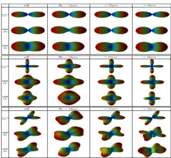
The proposed method was evaluated on different types of MR images with different radial sampling schemes and different sampling ratios and compared with the state- of-the-art

In this paper, based on the Riemannian framework for ODFs /EAPs and Spherical Polar Fourier (SPF) basis represen- tation, we propose a unified model-free multi-shell HARDI method,

In this paper, we have proposed a novel compressed sensing framework, called 6D-CS-dMRI, for reconstruction of the continuous diffusion signal and EAP in the joint 6D k-q space. To