An advanced time-dependent queueing model for airport delay analysis

I

AN ADVANCED TIME-DEPENDENT

QUEUEING MODEL

FOR AIRPORT DELAY ANALYSIS

Emily Roth

Report FTL-R-79-9

October 1979

Emily Roth

FTL Report R79-9 October 1979

Flight Transportation Laboratory Massachusetts Institute of Technology

Acknowledgement

I am very grateful to Professor Amedeo R. Odoni for his guidance in this research and for his detailed com-ments and suggestions on this paper.

TABLE OF CONTENTS

Table of Contents ... List of Figures ...

Section 1. Introduction ...-Section 2. The Models ...

2.1. The Basic Model ...--2.1.1. Definition of Terms ... 2.1.2. Priority Schemes... 2.1.3. Notation ... 2.1.4. State Equations and Performance

Measures ... 2.1.5. The Computer Program ... 2.2. The Extended Model...

2.2.1. Notation ... -2.2.2. State Equations and Performance

Measures ...--Section 3. Experimental Results

...-...--3.1. Verification ... 3.2. Using the Extended Model ...

Section 4. Expected Delay

...--4.1. Alternating Priority...--4.2. Strict Type 1 Priority ... Section 5. Extensions and Conclusions ...

Appendix ,P---.. ---. References ... 61 Page 11 56 ... 0 .. 0 . . -... 0

-iii-LIST OF FIGURES Figure Figure Figure Figure 3-1: 3-2: 3-3: 3-4: Figure 3-5: Figure 3-6: Figure 3-7: Figure 3-8: Figure 3-9: Figure 3-10: Figure 4-1: Figure 4-2: Figure 4-3: Figure A-1: Page Demand Profiles for Test Cases 1-4 ... 28

Expected Number of Aircraft in Queue for Test

Cases 1-4 ... 30 Demand Profiles for Test Cases 5 and 6 ... 32

Expected Number of Aircraft in Queue for Test

Cases 5 and 6 ... 33 Demand Profiles for Simulation and Two-Queue

Models ... 35 Expected Number of Landing Aircraft in the

System - Strict Type 1 Priority ... 36 Expected Number of Departing Aircraft in

Queue - Strict Type 1 Priority... 37 Expected Number of Aircraft in Each Queue for the Basic and Extended Models - Alternating Priority. 39 Expected Number of Landing Aircraft in the

System - Extended Model ... 41 Expected Number of Departing Aircraft in the

System - Extended Model ... 42 Expected Delay Under Alternating Priority for

Three Levels of Runway Utilization ... 48 Expected Delay to Landing Aircraft - Strict

Type 1 Priority ... 52 Expected Delay to Departing Aircraft - Strict

Type 1 Priority ... 53 State Transition Diagram for Basic Model - Alter-nating Priority ... 57

In the past several years many attempts have been made to model the probabilistic nature of airport runway operations using a queueing-theoretic approach to runway modeling. Early studies were limited by computational considerations to examination of systems only once they reached "steady state". These models were unable to reflect the characteristic hourly "rises" and "falls" of demand for runway use at major airports. Koopman [4] was the first to include time-varying de-mand in a queueing model of a runway. He examined simple M(t)/M/l and M(t)/D/1 models with planes awaiting landing or takeoff placed in a

single common queue. By using advanced numerical techniques he showed that the airport system equations can be solved recursively through the computer to exhibit the system behavior as a function of time. A later study by Hengsbach and Odoni [3] extended these models to include the case of k independent runways. This study also resulted in a set of computer programs which increased tremendously the computational effi-ciency of this approach.

In this report we explore, for the first time, time-dependent queueing-theoretic models in which landing and departing aircraft are kept in separate queues. This allows explicit acknowledgement of

various sequencing strategies by air traffic controllers and computation of separate statistics for delays to landings and to takeoffs.

The report is organized into several basic sections. Expanding on an idea introduced by Koopman [4], we begin with the development of a basic two-queue runway model under time-varying demand. We then

-2-present an extended model which more realistically reflects actual air-port runway situations. Third, results from an experimental investiga-tion with these models are presented, including comparisons with the earlier single-queue model. Section 4 is a discussion of the expected delay to aircraft in these two-queue systems. Finally, we mention some simple extensions and suggest directions for further study.

2. The Models

This section discusses the two theoretical models examined in this report and includes a brief description of the computer program used to solve them. The "basic model" is a straightforward, two-queue inter-pretation of an airport runway but provides only a rough representation of operations at most airports. The "extended model", although substan-tially more costly to implement, can portray mixed operations on single runways with much more accuracy and can also be used to model selected intersecting runway situations (see Section 3.2).

2.1 The Basic Model

The basic model is an extension of an M(t)/M/l queueing system to account for two types of "customers" (aircraft to land or to takeoff) with different demand and service characteristics, and sequenced by various priority schemes.

Aircraft arrive in a probabilistic manner to land and are directed into a queue (holding stack) in the air if the runway is occupied. Meanwhile, other aircraft queue up next to the runway awaiting takeoff. Arrivals to each queue are assumed to be statistically independent

Poisson processes with time-varying average arrival rates. Once an air-craft enters a queue it maintains its position ensuring come, first-serve treatment within each queue.

The runway is a single server, serving both types of aircraft in a nonpreemptive manner. The length of service for any aircraft is the total time it occupies the final approach/runway sequence, thus preventing

-4-other waiting aircraft from being served. This service time is probabi-listic with a general probability distribution. Past examinations of the single-queue model [3,4] have shown the system to be quite insensitive to the exact form of this distribution under the particular demand pro-files characteristic of major airports. This allows the analysis to be immensely simplified by assuming that service times are exponentially distributed. We further simplify the model by specifying that each of the two aircraft types has its own, time-independent average service rate.

2.1.1 Definition of Terms

For convenience, aircraft waiting to land are denoted as "type 1" and the queue that these aircraft form (often in holding stacks) is "queue 1". Aircraft waiting for a takeoff are "type 2" and the ground queue is referred to as "queue 2".

The "system" we are concerned with consists of the runway and the two queues of aircraft awaiting runway use. The "state of the system" is defined by an ordered set of numbers. State (I,J,K) represents I-1 type 1 and J-l type 2 aircraft in the system with a type K (K = 1,2) aircraft in service (the indices are shifted by 1 to maintain consistency

*

with the computer terminology).

Since the number of equations (or equivalently the number of states) describing the system must be finite to be soluble, maximum queue sizes must be specified. This means that any aircraft arriving to a full queue will be turned away and hence lost from the system. Care must be

taken to choose these maximum lengths large enough to avoid turning away any aircraft in the course of any normal day's operations.

The physical capacity of the system can be specified either by the total number of spaces in queue or the total number of aircraft

in the system. We have chosen to use the latter definition. This im-plies that the capacity of each queue is a function of the type of air-craft in service. To avoid ambiguity, care must be taken with termi-nology. For instance, "number in queue" does not include the customer

in service. Also, the term "arrival" refers to an aircraft of either type entering the system rather than to landing aircraft.

2.1.2 Priority Schemes

As the runway serves two types of "customers", the type of air-craft to next begin service each time the runway is vacated, must be determined by a set of priority rules. In this work we have examined

four different priority schemes which are described below.

The "strict type 1" scheme gives absolute priority to type 1 aircraft. In other words, whenever the runway becomes free, type 1 planes are given preference on a FCFS basis. If queue 1 is empty, the first aircraft in queue 2 is directed to begin its takeoff.

In the "alternating" scheme, as soon as an aircraft completes service, one of the other type, as long as such an aircraft exists, will be given preference to next use the runway.

-6-The "strict type 1/strict type 2" and "strict type 1/alternating" schemes combine two sets of priority rules. In each, as long as the num-ber of type 2 aircraft in the system remains at or below an arbitrary threshold (called MCUT), type 1 aircraft are given strict priority. If, however, the number of type 2 aircraft exceeds MCUT, the rules change, either by giving type 2 aircraft strict priority or by switching to al-ternating priority. In each case, as soon as there are MCUT or fewer type 2 aircraft in the system, type 1 planes are once again given absolute priority.

In summary, the schemes are outlined below: - strict type 1: absolute priority given to type 1.

- alternating: priority is given to the type other than the one which last completed service.

- strict type 1/strict type 2: if MCUT or fewer type 2 aircraft are in the system, preference is given~ to type 1. If the number of type 2 exceeds MCUT, absolute priority is given to type 2 aircraft.

- strict type 1/alternating: as in strict type 1/strict type 2, except that, if the number of type 2 aircraft exceeds MCUT, alternating priority is imposed.

2.1.3 Notation

We have chosen to make our notation slightly unnatural in order to eliminate the need for three subscripts to the state variables. Note also that explicit time dependence has been suppressed.

The parameters used are as follows:

Ni = maximum number of type 1 aircraft allowable in the system. N2 = maximum number of type 2 aircraft allowable in the system.

MN1 = Nl + 1.

MN2 = N2 + 1.

MCUT = changeover value for priority schemes involving a threshold. If there are less than or equal to MCUT type 2 aircraft in the system, one set of priority rules is followed; if the number of type 2 exceeds MCUT a different scheme is imposed.

The following variables are functions of time but this dependence has been suppressed in the variable names:

R = probability that the system is empty at time T. P(IJ) = probability that I-1 type 1 and J-1 type 2 aircraft

are in the system at time T and a type 1 aircraft is in service.

Q(I,J) = probability that 1-1 type 1 and J-1 type 2 aircraft are in the system at time T and a type 2 aircraft is in service.

DR = rate of change of R at time T. DP(I,J) rate of change of P(I,J) at time T. DQ(I,J) = rate of change of Q(I,J) at time T.

Ll = average arrival rate to queue 1 at time T (Ll = X (T) in conventional queueing theory notation).

L2 = average arrival rate to queue 2 at time T (L2 = X2(T)), Ul = average service rate of type 1 aircraft at time

T (Ul = y1().

U2 = average service rate of type 2 aircraft at time T (U2 = P2

-8-2.1.4 State Equations and Performance Measures

The state equations are first-order differential equations describing the rate of change of the number and position of each type of aircraft in the system as a function of time. These equations, derived by techniques described in the appendix, are sparse but numerous. Each of the priority schemes entails solving a set of these simultaneous, first-order equations. The number of equations is given by N = 2(MNl)(MN2) + 1. For example, if we allow a maximum of 15 aircraft of each type in the system, N is already equal to 513.

On the next several pages we provide computer listings of the state equations for each of the priority schemes described in Section 2.1.2.

Solving the system of differential equations will yield the state probabilities as a function of time. These can in turn be used to obtain statistics to describe system behavior.

We have examined quantities such as the following (the time dependence has been suppressed):

(i) The probability that a type 1 aircraft is in service at time T, MNl MN2

PROB = Z E P(IJ) I=1 J=1

(ii) The probability that a type 2 aircraft is in service at time T, MN1 MN2

PROB2 = Z E Q(I,J)

State Equations for the Rasic Model - Strict Type 1 Priority DR=-(Ll*L2)*R+UI*P(29l)*U2*U(1*2) DP(291)=-(LI+LZ+Ul)*P(2*L)*Ll*R+UIOP(J9l)*U2*0(292) 00 140 1239NI DP(191)=-(Ll*L2*01)*P(191)+LI*P(I-191)*UI*P(l*l9i)+U2*0(1*2) 00 130 J=29N2 130 OP(ItJ)=-(Ll-L2*01)*P(19J)+LI*P(I-I-PJ)*L4d*P(19J-L)+UI*P(I*lqj) -#u2*U(IVJ*I) 120 DP(19MN2)=-(LI*Ul)*P(lm42)*LI*P(T-19ON2)*L2*P(l9N2)*Ijl*P(I*lgMN2) OP(MNJ*1)=-(L2-Ul)*P(mNlgl)+LI*P(Nlgi)+Ue*Q(MNIge) DP(29MN2)=-(LI+Ul)*P(P*MNe'4L2*P(29 le)*UI*P(39MNd) DO 140 J=29N2 OP(29J)=-(Ll+L2*Ul)*P(29J)#L2*0(29J-L)*UI*P(39J)*U2*()(29J*l) 140 OP(MN19J)=-(L2+Ul)*P(MN19J)*LIOP(NI*J)*Ld*P(MN19J-I)*t)2*0(MN19J+l) DP(MN19MN2)=-UI*P(MNIMNe)*Ll*P(NI*MNd)*Le*P(MNl9N2) DO 170 1329NI 00(192)=-(Ll+L2+U2)*O(Iqe)+LI*O(I-lqe) DO 160 J=3*N2 180 0(4(1-DJ)=-(Ll*L2*u2)00(1,J)*Ll*O(I-IPJ)*Ld*o(lqj-l) 170 DO(IoMN2)=-(Ll*U2)*O(TMN2)+Ll*0(1-1,MN2)*L2*Q(l9N2) DQ(192)=-(Ll+L2+U2)*Q(I.d)+L2*R+UI*P(e92)*U2*0(193) DO 190 J=39N2 DO(MNI*J)=-(L2+U2)*O(MN19J)*Ll*G(NlgJ)+Ld*Q(MNloJ-1) 140 DO(19J)=-(Ll+L2*U2)*O(J*J)*L2*0(19J-L)+UL*P(2*J)*U2*0(19J+I) DO(MN192)=-(L2+U2)OO(MN192)+LI*O(NI92) DO(19MN2)=-(LI*IJ2)00(1-PM'4,e)*L2*0(1*Ne)*UI*P(2*MNd) OO(MNI*MN2)=-U2*0(MN19MNe)+LJ*Q(NltMN4)+Le*Q(MNl9N2)

-10-State Equations for the Basic Model - Alternating Priority

DR=-(Ll+L2)*R*UJ*P(2tl)*U2*U(192) DP(291)=-(Ll+L2*Ul)*P(2-1)*LI*R*UJ*P(J9l)+U2*0(292) DP(MN191)=-(L2*(Jl)*P(MNIti)*LI*P(Nltl)*Ue*Q(MN19e) DG(192)=-(Ll*L2*U2)*0(192)+L2*R*UI*P(e92)*U2*0(193) Do 110 J=3*N2 DO(MN19J)=-(L2*U2)*Q(MN19J)*Ll*G(NltJ)+Le*G(MN19J-1) 110 DQ(IOJ)=-(Ll+L2+U2)*0(19J)*L2*0(1*J-I)*UI*P(29J)+U200(loJ#l) DO(loMN2)=-(Ll+U2)*0(19MN2)*L2*0(1*Ne)+UI*P(29MNe) DO(MN192)=-(L2*U2)*Q(MN192)+LI*Q(Nlgd) Do 1JO J=2*N2 DP(MNJ*J)=-(L2*Ul)*P(MN19J)+LI*P(NloJ)+LZ*P(MN19J-I)+ Ue40(MNj.J+J) 130 DP(2*J)=-(Ll*L2+Ul)*P(2tJ)*L2*P(29J-I)*Ue*0(2*j+i) DP(29Mt42)=-(LI+Ul)*P(2*MV?)+L2*P(29Ne) Do 140 1=39NI DO 150 Jz2,N2 150 DP(IgJ)=-(Ll*L2*Ul)*P(19J)+LI*P(1-1*J)+LZOP(19J-I)-U2*0(I*J+l) DP(19MN2)=-(Ll+Ul)*P(TeMN4)+Ll*P(T-liMN2)*L2*P(l9N2) 140 DP(I-Pl)=-(Ll*L2+Ul)*P(Iti)#LI*P(I-l-pl)+Ul*P(l#l-pl)+U2*0(102) DP(MNI*MN2)=-Ul*P(MN19MN2)*Ll*P(NlqMNe)+Le*P(MNl9N2) DO 180 1=2,N1 DO 190 J=39N2 190 DO(19J)=-(Ll*L2*IJ2)*O(IqJ)*Ll*O(I-ltJ)*L?*0(19J-i)+Ul*P(1+19J) DO(I92)=-(Ll+L?-U2)*Q(Ige)*Ll*O(l-lve)*UI*P(I+Ige) 180 DQ(I*MN2)=-(Ll+U2)*G(IMNe)*Ll*0(1-19MN2)#L2*O(l9N2)*L)1*P(1*1*MN2) DO(MNIoMN2)=-U2*0(MN19MN2)*LI*G(NltMNe)*Le*O(mNl9N2)

State Equations for the Basic Model - Strict Type l/Strict Type 2 Priority MCUTI=MCUT*l MCUTe=MCUT+2 DR=-(Ll*L2)*R+UI*P(29l)*J2*0(192) DP(MN191)=-(L2*Ul)*P(MN191)*LI*P(Nloi)*Ue*O(MNlee) DO(192)=-(Ll*L2*U2)*0(1*2)*L2*R+UI*P(e92)*U2*0(193) DO 110 Jz3,N2 110 DQ(1*J)=-(Ll*L2*U2)*0(19J)*L2*0(lgj-i)*UI*P(29J)*U2*0(19J*I) DP(291)=-(Ll*L2+Ul)*P(291)*LI*R*UIOP(J9l)*U2*0(292) DO 1b0 IZ39N1 Do 160 J=29MCUTI 160 DP(19J)=-(Ll#L2*Ul)*P(I*J)+Ll*P(I-19J)+Le*P(I*J-i)#U2*0(19J*I) - +UI*P(I*Itj) DO 190 JzMCUT2vN2 190 DP(19J)=-(Ll*L2*Ul)*P(IgJ)*Ll*P(I-19J)+Le*P(19J-1) DP(Itl)=-(LI+L2*Ul)*P(191)*LI*P(1-191)+Ue*0(192)*UI*P(1*191) 150 DP(I*MN2)=-(Ll*Ul)*P(19MNe)+LI*P(T-leMN2)*L2*P(l9N2) DQ(I*MN2)=-(Ll+U2)*0(19MN2)+L2*0(IoNe)*UI*P(2,MNe) DO(MN192)=-(L2*U2)*Q(MN192)*LI*G(Nloe) DP(29MN2)=-(Ll*Ul)*P(29MNe)+L2*P(2oN2) DP(MN19MN2)=-UI*P(MN19MN2)+LIOP(NlgMNe)*Le*P(mNl9N2) Do 170 J=29MCUTI DP(29J)=-(Ll*L2+Ul)*P(29J)#L2*P(29J-I)+UI*P(39J)*U2*0(2*J#I) 170 DP(MN19J)=-(L2*Ul)*P(MN19J)*Ll*P(NIJ)*Le*P(MN19J-l)+U2*0(MN19J*I) DO 2bO 1=29N1 Do 260 J=MCUT2.,N2 260 DO(19J)=-(Ll*L2*U2)*0(19J)*Ll*0(1-1*J)*Le*0(19J-I)*UIOP(I*19J) +U2*0(I*J*I) DO 230 J=3*MCUT1 230 DO(IOJ)=-(Ll+L2*U2)*0(19J)*LI*0(1-19J)+Le*0(19J-1) DO(192)=-(Ll+L2+U2)*0(192)+Ll*O(l-lge) 2!>O DO(IgMN2)=-(LI*U2)*G(TiMN2)*Ll*Q(l-lsMN2)*L2*G(l9N2)*UIOP(1*1OMN2) DO 240 J=3*MCUTI 240 DO(MNlgj)=-(L2*U2)*Q(MN19J)*LI*G(NI*J)*Le*G(MN19J-1) DO 270 J=MCUT29N2 DP(29J)=-(Ll*L2*Ul)*P(29J)+L2*P(29J-1) DP(MN19J)=-(L2*Ul)*P(MN19J)*LI*P(NlqJ)*Le*P(MNI*J-1) 270 DO(MN19J)=-(L2*U2)*Q(mNl*J)*Ll*Q(NloJ)*Le*O(MNIJ-I)*1)2*0(MN19J+I) DO(MNI#MN2)=-U2*0(MNI.MN2)*LIOO(NI*MNe)*Le*O(MNltN2)

State Equations for the Basic Model - Strict Type l/Alternating Priority L3=L2 MCUTI=MCUT*l MCUT2=MCUT+2 DP=-(Ll+L2)*R*Ul*P(291)-J2*Q(lo2) DP(2tl)=-(LI+L2+Ul)*P(2,i)+Ll*P*UI*P(J-l)*U2*0(292) DO leO 1=3.Nl DP(Itl)=-(Ll+L2+Ul)*P(191)*Ll*P(I-191)*UI*P(l*loi)+U2*0(1*2) DO IJO J=29MCUT 130 DP(ItJ)=-(Ll*L2*Ul)*P(I*J)*LI*P(I-19J)+Le*P(19J-I)+UI*P(I*19J) -+L)Z*U (1 9 J+ I ) DP(19MCUTI)=-(Ll*L3*(Jl)*P(I*MCIJTI)*Le*P(I*MCUT)#LI*P(I-19MCUTI) - *U2*Q(1*mCUT2)+UI*P(I+19MCUT1) DO 135 J=mCUT2,N2 135 DP(IOJ)=-(Ll*L3#Ul)*P(I*J)+LI*P(I-1*J)*LJ*P(ItJ-l)#U2*0(I*J*I) 120 DP(I*Mt42)=-(Ll+Ul)*P(79M'4e)*Ll*P(1-1*mN2)+L3*P(loN2) DP(MN191)=-(L2+Ul)*P(MNlql)*LI*P(Nll)*Ue*Q(MN19e) DP(29MN2)=-(LI*Ul)*P(?qMNe)*L3*P(2*Nd) DO 140 J=2e4CUT DP(2*J)=-(Ll+LP*Ul)*P(2*J)*L2*P(2*J-I)+UI*P(3*J)*U2*0(29J*I) 140 DP(MN19J)=-(L2+ul)*P(MNIOJ)+LI*P(NlgJ)+Le*D(MNI*J-I)+U2*0(MN19J*I) DO 148 J=39MCUT DQ(1,J)=-(Ll*L2*U2)*0(19J)*L2*0(1,J-1)*UI*P(29J)*UP*0(1*J+l) 148 DO(MN19J)=-(L2*U2)*Q(MN19J)*Ll*O(NI*J)+Le*Q(MN19J-1) DO 145 J=MCUT2*N2 DP(MN19J)=-(L3*Ul)*P(MN1,J)*Ll*P(NI*J)+LJ*P(MN19J-I)+ - U2*0(MN19J*l) DO(19J)=-(Ll*L3+U2)*0(1*J)*L3*0(1*J-I)#UI*0(2*j)*U2*0(19J+l) DO(MNlgj)=-(L3*U2)*Q(MN19J)+LI*O(NloJ)*LJ*Q(MN19J-1) 145 DP(29J)=-(LI*L3+(Jl)*P(29J)+L3*P(2*j-l)*Ue*0(29J-1) DP(MN19MN2)=-01*P(MN19MN2)*Ll*P(NlgMNe)*LJ*P(MNloN2) DO 170 I=2*Nl Do(192)=-(LI+L2+LJ2)*0(1*2)*Ll*O(I-Ioe) Do 160 J=3*MCUT 180 DQ(19J)=-(Ll*L2*U2)*Q(I*J)#LIOQ(1-19J)*Ld*O(I*J-1) DO(IqMCUT1)=-(Ll#L3*iJ?)*U(l*MCUTI)+Le*0(19MCUT)+LI*0(1-19MCUTI) Do 195 J=mCUT?9N2 195 DQ(I*J)=-(Ll+L3+LJ2)*Q(I*J)+Ll*Q(I-I*J)*LJ*Q(IJ-I)+UI*P(1*19J) 170 DO(IoMN2)=-(Ll+U2)*0(79MNd)*Ll*O(I-1,MN2)+L3*0(1,N2)+UIOP(1*19MN2) DQ(192)=-(Ll*L2+tJ2)00(loe)+L2*P*UI*P(e92)*U2*0(193) DO(MNlp2)=-(L?*(J2)*Q(MN112)+Ll*Q(Nlte) DP(29MCUTI)=-(Ll*L3#Ul)*P(29MCUTl)+L2'P(e*MCUT)+U2*0(2,MCLIT2) - +Ul*P(39MCUT1) DP(MN19MCUT1)=-(L3*Ul)*P(MN19MCUT1)*Le*P(MNI*MCUT)+U2*0(MNIgmCUT2) - *L I *P(N I 9MCLIT I) DO(MN19MCUTI)=-(L3*U2)*O(MN19MCUTJ)*Ld*Q(MN19MCUI)+Ll*O(NIoMCUTI) DQ(19MCUTI)=-(Ll#L3+U2)*U(19MCUTI)+Le*0(19MCUT)*Ul*P(2*mCt)Tl) - +Ue*U(194CUT2) DQ(19MN2)=-(LI*U?)*0(19MN2)*L3*Q(lqNe)*UI*0(2oMNe) DO(MN19MN2)=-U2*0(MN19MN2)*Ll*Q(NloMVe)*LJ*O(MNltN2)

(iii) The expected number of type 1 aircraft in the system at time T,

MN1 MN2

ELl = E (I-1)[P(I,J) + Q(I,J)] I=1 J=1

(iv) The expected number of type 2 aircraft in the system at time T, MN1 MN2

EL2 = E E (J-1)[P(I,J) + Q(I,J)]. I=1 J=1

(v) The expected number of aircraft in queue 1 at time T, MN1 MN2

EQl = E [(I-2)P(IJ) + (I-1)Q(IJ)]. 1=1 J=l

(vi) The expected number of aircraft in queue 2 at time T, MNl MN2

EQ2 = E [(J-1)P(I,J) + (J-2)Q(I,J)]. I=1 J=l

(v) The total expected number of aircraft in queue at time T,

EQ = EQl + EQ2.

2.1.5 The Computer Program

To solve the systems of simultaneous, first-order differential

*

equations, the computer program included an IMSL subroutine named DVOGER. This program is written in double - precision FORTRAN and uses Gear's Method to recursively obtain the state probabilities as a function of time. The time increment between successive iterations is variable,

*

-14-chosen just small enough by DVOGER to satisfy a specified one-step error criterion.

In addition to the equations, inputs to the computer program include the average demand and service rate profiles for each type of aircraft. The state probabilities obtained as outputs can be used to compute statistics such as those discussed previously.

A discussion of computation time and cost is contained in Sec-tion 5.

2.2 The Extended Model

Although the basic two-queue runway model is much more powerful than the single-queue model, it is still not sophisticated enough to provide a realistic picture of air traffic congestion in many practical situations. Specifically, recall that in this basic model the average service rates depend solely upon the type of aircraft currently in ser-vice. In practice, however, aircraft service times on runways are also highly dependent upon the type of aircraft previously using the runway.

For instance, under Instrument Flight Rules (IFR), when a landing is preceded by a takeoff on the same runway, the landing aircraft can be as

close as 2 n. miles from the runway at the time when the takeoff roll be-gins. By contrast, if the preceding operation is also a landing, a mini-mum separation of 3-6 n. miles (depending on aircraft weights) is

re-quired. Thus, the "time-gap" between successive operations, i.e., the service time for the landing, depends on whether the preceding operation is a landing or a takeoff.

A quite straightforward extension of the basic model takes account of dependence on the type of the previous aircraft in service by label-ing each state with four indices: state (I,J,K,L) represents I-1 type 1 and J-1 type 2 aircraft in the system, a type K (K=1,2) customer currently in service and a type L (L=0,1,2) customer last in service

(L is set to zero if the current aircraft arrived to find an idle runway). Average service rates are now specified by pKL where K is the type of aircraft currently in service and L is the type previously served.

-16-2.2.1 Notation

The modified notation for this model follows. For complete-ness, notation common to both models has been repeated.

For the extended model the parameters are:

N1 = _{maximum number of type 1 aircraft allowable in the system.}

N2 = _{maximum number of type 2 aircraft allowable in the system.}

MN1 = N1 + 1.

MN2 = N2 + 1.

MCUT = _{changeover value for threshold priority schemes.}

The variables are (time dependence suppressed):

R = _{probability that the system is empty at time T.}

PL(I,J) = _{probability that I-1 type 1 and J-1 type 2 aircraft}

are in the system at time T, a type 1 is in service and a type L (L=0,l,2) just completed service. QL(I,J) = _{probability that I-1 type 1 and J-1 type 2 aircraft}

are in the system at time T, a type 2 is in service and a type L (L=0,1,2) just completed service. DR = rate of change of R at time T.

DPL(I,J) = _{rate of change of PL(I,J) at time T (L=0,1,2).} DQL(I,J) = rate of change of QL(IJ) at time T (L=0,1,2). Ll = _{average arrival rate to queue 1 at time T (L1 = X}

1(T)).

L2 = _{average arrival rate to queue 2 at time T (L2 = 2 (T)).}

UKL = _{average service rate of a type K aircraft which was}

2.2.2 State Equations and Performance Measures

Due to the increased complexity in the definition of a state, the state equations for the extended model are less sparse than those of the basic model but they are derived and solved in the same manner. The equations for the four priority schemes discussed in Section 2.1.2 are listed on the next several pages.

At time T, the corresponding statistics for the extended system are: MNl (i) PROB1 = I=1 MN1 (ii) PROB2 =

Z

[PO(I,J) + Pl(IJ) + P2(IJ)].

[QO(I,J) + Ql(IJ) + Q2(IJ)].

(I-1)[PO(I,J) + Pl(I,J) + Ql(IJ) + Q2(IJ)]. (J-1)[PO(I,J) + Pl(I,J) + Ql(IJ) + Q2(IJ)]. + P2(IJ) + QO(IJ) + P2(I,J) + QO(I,J) MN1 MN2

(v) EQl = E [(I-2)(PO(IJ) + Pl(I,J) + P2(IJ)) I=1 J=l

+ (I-1)(QO(I,J) + Ql(IJ) + Q2(I,J))]. MN1 MN2

(vi) EQ2 = Z [(J-1)(PO(I,J).+ Pl(I,J) + P2(I,J)) I=1 J=1

+ (J-2)(QO(I,J) + Ql(I,J) +

Q2(IJ))].

-18-State Equations for the Extended Model - Strict Type 1 Priority

DP=-(Ll*L2)*R*UlO*PO(Ptl)*Ull*Pl(2*1)+Llld*P2(2*l)*U20000(192) - *U21*Q1(192)+U22*Q2(192) DPO(doi)=-(Ll*L2+UIO)OPO(291)*LI*R DPI(eol)=-(Ll+L2*Ull)*Pl(Loql)#ijlo*Pn(jol)*ull*PI(391)*()12*P2(391) DP2(291)=-(Ll*L2+UI2)*P2(d9l)*U20*00(e*2)*U21*01(292)*t)22*Q2(2*?) DO 120 1=3oNl DPO(191)=-(Ll+L2#UIO)*PO(191)+Ll*PO(1-191) DPI(191)=-(Ll#L2+Ull)*PI(191)#LI*PI(I-191)+UID*PU(1*191) DPZ(191)=-(Ll+L2*Ul2)*P2(191)+LI*P2(1-191)*L)20*OU(I92) +U21*Q1(192)*U22*Q2(I9,d) Do 1JO J=2*N2 DPO(19J)=-(Ll*L2*UIO)*PO(I*J)*LI*PO(1-1*J)*L2*PO(I*J-1) DPI(19J)=-(Ll+L2-Ull)*PI(I*J)+Ll*PI(1-19J)*L2*PI(IJ-1) *UIO*PO(1*19J)*UII*Pl(l+l*J)*LJ12*,Ie(1*19J) 130 DP2(19J)=-(LI+L2+UI2)*P2(19J)*LIOP2(1-1*J)*L2*P2(19J-1) - *U20*UO(Igj4l)*L)21*01(19J*1)41)22*,Je(loJ*I) DPO(19MN2)=-(LI+UIO)*PO(19MN2)+LI*PO(i-l9mt42)*L2*PO(loN2) DP1(19MN?)=-(LI+Ull)*Pl(lgtIN2)*LI*Pl(l-l9m42)+L2*Pl(loN2) - *UlO*PO(1#19MN2)*UII*PI(1+1*MN2)*JI20v?(I*lgMN2) 120 DP2(19MN2)=-(LI*UI2)*P2(leMN2)+LlOP2(i-leMN2)#L2*P2(l9N2) DPO(MNltl)=-(L2#UIO)*PO(MNI91)*LI*PO(Nlol) DPI(MN191)=-(L2*Llll)*Pl(4NI91)*LI*PI(Nlgl) DP2(.%IN1*1)=-(L2-t)12)*P2(1414191)+Ll*P?(Nlol)*020*OU(MN192) - +U21*UI(MN192)+U22*Q2(MN192) DPO(29MN2)=-(LI+UlO)*PO(29MN2)*L2*PO(ieNd) DPI(egMN2)=-(LI+Ull)*Pl(eoMN2)+L2*Pl(,4,,Ne)*UlO*PU(39MN2) - *U11*P1(39mN2)*U12*P2(39mN2) DP2(eqMN2)=-(Ll+l )12)*P2(egMN2)*L2*P2(d*Nd) Do 140 J=29N2 DPO(dgJ)=-(Ll*L2+UIO)*PO(29J)-L2*PO(e*J-1) DP1(eoJ)=-(Ll*L2-Ull)*Pl(?tJ)*L2*Pl(e#J-I)+IjlO*PU(39J) - *U1I*PI(39J)+U12*PP(39J) DP2(dgJ)=-(Ll*L2*Ul2)*P2(Z*J)#L2*P2(eoJ-I)*()20*QU(29J*I) - +U21*Q1(29J#I)+U22*Q2(29J*I) DPO(MN1*J)=-(L?*UlO)*PO(MN19J)+LIOPO("419J)*1-2*PO(MNI*J-1) DP1(MN19J)=-(L?+t)ll)*Pl(4NIgj)+LI*Pl(t4lgJ)*L2*Pl(mNlgj-l) 140 DPZ(MN19J)=-(L2*1312)*P2("NloJ)*LI*P2(oljl*J)*L2*P2(MN19J-1) - *U20*00(MNI*J*1)+(J?1*JI(MN19J*I)+U42*Ue(MN19J*I) DPO(MN19MN2)=-LJID*PO(MN19MNd)*Ll*PO('YI.PMNd)*L2*PO(MNloN2) DPI(MN19MN2)=-tlll*Pl(MN19MN2)+Ll*PI(NlgMN-)*L2*Pi(MNl9N2) DP2(mNlgMN2)=-IJ12*P2(MNloMN2)*LI*P2(vlgMNe)+L2*Pe(MNloN2) 00 170 1=2oNl DGO(192)=-(LI+L2+U20)*QO(IgZ)*LI*GO(1-19e) DOI(192)=-(Ll*L2*U21)*01(192)*Ll*Ql(1-loe) DQZ(192)=-(Ll+L2*U22)*02(1*2)#LI*Q2(1-ltd) Do 1dO Jz3*N2 DQO(19J)=-(Ll#L2*U20)*00(1*J)+LI*00(1-19J)+L2*00(IgJ-1) Dol(I*J)=-(Ll*L2+U21)*01(IgJ)*LI*01(1-19J)+L2*Ql(I*J-1) 180 D02(19J)=-(Ll+L2+1)22)*02(19J)*Ll*02(1-1*J)*L2*02(1*J-1) DQO(19MN?)=-(LI+U20)*00(19MN2)+LI*00(i-lgMN2)*L2*Qn(loN2) DQI(19MN2)=-(LI+U21)*01(19MN2)*LI*01(1-19MN2)-L2*01(I9N2) 170 D02(1*MN2)=-(LI+LJ22)*02(19MN2)*Ll*02(i-loMN2)+L2*Q2(I9N2) DOU(192)=-(Ll*L2*U20)000(19e)*L2*P Dol(l92)=-(Ll+L2+U21)*QI(192)*tjlO*PO(-'92)*tjll*Pl(292)*()12OP2(2*?) D02(192)=-(Ll+L2+U?2)*02(ige)*1)20000(193)+L)21*01(1*3)*u22*Q2(193) DO 190 J=39N2 DOO(MN19J)=-(L2*U20)*00(4NIgj)+Ll*00(Nl9j)*L2*00(MNI*J-1) DOI(MN19J)=-(L2+U21)*01(4Nl9J)+LI*01(NlgJ)+L2*Ql(MN1*J-1) D02(MN1*J)=-(L2*LJ22)*02(41419J)*LI*02(1'41-)J)+L2*02(MN1-PJ-1)

DOI(MNIte)=-(L2#U21)*01(4NI92)+LI*Ql(Nlge) D02(MN192)=-(L2+U22)*02(4NI92)+LI*02(Nlge) DOO(leMNZ)=-(LI+U20)*00(1*MN2)+L2*0O(ItNe) [)01(19MN2)=-(Ll*U21)*01(19MN2)*L2*01(ioNd)*UlO*PU(29MN2) - +UII*Pl(29MN2)+Ul2*P2(29MN2) D02(loMN2)=-(Ll*U22)*02(19MN2)*L2*02(itNe) DOO(MN19MN2)=-U20*00(MN19MN2)+LI*00(NIeMN2)+L2*GU(MNl9N2) DOI(MNliMN2)=-U21*01(MNltmNZ)+LI*01(NloMfqe)+L2*QI(MNItN2) D02(MN1*MN2)=-tj22*02(mNleMN2)+LI*02(NioMNd)+L2*Qe(MNl9N2)

-20-State Equations for the Extended Model - Alternating Priority

DP=-(Ll*L2)*R+IJIO*PO(?*I)+Ull*PI(2*1)*Ule*02(291)*U20*00(I-o?) +U21*UI(I*2)*LI22*02(Ie) OPO(eol)=-(Ll#L2#UlO)*PO(eol)#Ll*R DPI(491)=-(Ll*L2*Ull)*Pl(291)+ijlo*Po(-Iol)*ull*PI(391)+UI2*P2(391) OP2(291)=-(Ll*L2,PU12)*P2(,doi)+i)20*00(492)*U21*Ql(2e2)*1)22*02(297) DO 120 1=3*Nl OPO(Iol)=-(Ll*L2#UJO)*PO(191)+Ll*PO(I-Igi) DPI(191)=-(Ll+L2+Ull)*Pl(ltl)+LI*PI(L-191)*()10*PU(1#191) DP.e(lol)=-(LI*L2+Ul2)*P2(191)*LI*P2(l-l9l)+U20*OU(192) +U21*U1(I92)+U22*02(I9e) 00 1JO J=29N2 OPU(19J)=-(Ll+L2*UIO)*PO(19J)+LI*PO(1-1*J)+L2*PO(19J-1) OPI(19J)=-(LI*L2*Ull)*P1(19J)+LI*PI(I-I*J)*L2*PI(IOJ-I) 130 DP4(19J)2-(LI+L2+UI2)*P2(19J)-Ll*P2(1-1,J)+L2*P2(19J-1) - *U20*00(loJ*l)+U21*01(lgJ+I)+U22*Je(IoJ*I) DPO(I*MNe)=-(LI*UIO)*PO(19MN2)#LI*P0(i-19MN2)+L2*PO(lN2) DPI(19MNe)=-(LI+Ull)*PI(19MN2)*Ll*Pl(l-19MN2)*L2*PI(19N2) 120 OP2(19MN2)=-(Ll#t)12)OP2(loMN2)*LI*P2(1-19MN2)+L2*P2(IoN2) DPO(mNlql)=-(L2*UlO)*PO(4NI#I)#LIOPO("4191) OPI(MNI*I)=-(L2+011)*Pl(14NI91)#LI*PI(NI*L) DPe(mNlol)=-(L2#UI2)*P2(4(4191)*LlOP2(Nltl)+1)20*QU(MNI*P) - +U21*UI(MNj,2)+U22*Q2(mNI,2) DPO(29MNZ)=-(LI4,IJ10)*PO(29M.N2)#.L2*PO(.evNie) OPI(doMN2)=-(LI*Ull)*PI(2oMN2)*L2*Pl(etNd) DP2(dgMNe)=-(Llot)12)*P2(dMN2)#L2*P2(eoNe) Do 140 J=2,N2 DPO(eoJ)2-(Ll*L2#UlO)*PO(doJ)*L2*PO(egJ-1) DPI(eqJ)=-(LI-L2*Ull)*PI(49J)+L2*Pl(doj-l) DPe(49J)=-(Ll*L2+Ul2)*P2(egJ)+L2*P2(dgJ-L)#(J20*QU(2*J+l) - +U21*UI(29J*I)+U22*Q2(29J+I) DPO(MN19J)=-(L2*UIO)*PO(MNloj)+Ll*PO(NltJ)+L2*PO(MN19J-1) DPI(MN1,J)=-(L2*Ull)*PI(4NI*J)+L2*Pl( IN19J-1)*Ll*PI(NI*J) 140 DPe(MNItJ)=-(L2+UI2)*P2(MN19J)*LI*P2(NlgJ)+L2*P2(MN19J-I) - *U20*UO(MNIJ*1)+1)21*UI(MN1*J*1)*Ue2*(Id(MN19JOl) DPO(MNI*MN2)=-(JIO*PO(mNlgmN.d)+LI*PO(NLqMNe)+L2*PU(MNl9N2) DPI(MN19MN2)=-1)11*PI(MN19MNd)+Ll*PI(NieMNd)*L2*PL(MNloN2) DP-d(MNIoMN2)=-IJ12*P2(MN19MNe)+LlOP2(NlgMN4)#L2*Pe(MNl9N2) Do 170 I=2.Nl DQO(192)=-(Ll+L2#U20)000(192)*Ll*OO(l-lge) Dol(1492)=-(Ll*L2*U21)*01(192)+LIOQl(I-Ite) - +UIOOPO(1+192)*tjll*Pl(l*lo2)*UI2*0e(1*1*2) D02(192)2-(Ll*L2*U22)*02(lte)+Ll*02(1-lge) 00 1dO J=3,N2 D,)0(19J)2-(Ll*L2+U20)*00(19J)+LI*00(1-19J)#L2*00(IgJ-1) DII(IoJ)=-(Ll*L2+U21)*Ql(19J)+LI*01(1-19J)*L2*QI(19J-1) - *UIO*PO(1*1,J)+ull*Pl(l+19J)+ul2*,Je(1*19J) 160 002(1*J)=-(Ll+L2+U?2)*02(1*J)*Ll*02(1-19J)+L2*02(IgJ-1) DOO(LoMNe)=-(LI+U20)*O0(19MN2)*Ll*QO(l-l9m42)*L2*GO(leN2) DOI(19MN2)=-(Ll+U21)*01(LgMN2)+LI*Olti-lgmN2)+L24QI(I.N2) - *UIO*PO(1*19MN2)*Ull*Pl(l+19MN2)+UI2*Pe(1*19MN2) 170 002(1*Mf 42)=-(Ll+U22)*02(19MN2)*LI*02(1-19MN2)+L2*02(l9N2) Dt)0(192)=-(Ll*L2+U20)*QO(i92)+L2*R DOI(192)=-(Ll+L2+u2l)*01(192)*1)10*Po(e*2)*ull*PI(2*2)+012*P2(2oP) D02(192)=-(Ll+L2+U22)*02(192)+tj2O*QO(i93)*U2l*Ql(lo3)+(122*02(lol) 00 190 J=39N2 DOO(MN19J)=-(L2*IJ20)*00(4NIgj)*LIOQO(NltJ)*L2*00(MN19J-1) Dk')I(MNI#J)=-(L2*t)21)*01(4NIoJ)+LIOOI("419J)+L2*QI(MN19J-1) D02(MN19J)=-(L2+022)*02(4NIgj)+Ll*l?(NlgJ)+L2*Q2(MN19J-1) DQO(19J)=-(LI*L2*U20)*00(19J)*L2*00(19J-1)

0( 2(MNIod)=-(L2*L)22)*02(4NI92)*LIO(12(Nloe) DOO(LgMNe)=-(Ll*U20)*00(19MN2)*L2*00(i*Nd) 001(leMN2)=-(Ll*U21)*01(19MN2)+L2*01(i*Ne)*UIO*PU(29MN2) +Ull*PI(29MN2)+Ul2*P2(e94N2) 002(l*MNe)=-(Ll*U22)*02(19MN2)*L2*(32(1*Nd) DOO(MNI*MN2)=-U20*00(mNlgMN2)*LI*QO(NigMNe)+L2*OU(MNl*N2) DOI(MNI*MN2)=-(121001(PAN19MN2)+LI*QI(NioMNid)+L2*01(MNloN2) 00e(mNlgmN2)=-u22*02(mNl*MN2)+LI*02(,'iitMr4d)+L2*0e(4NlN2)

-22-State Equations for the Extended Model - Strict Type l/Strict Type 2 Priority

MCUTL=MCUT*l MCUT2=MCUT*2 DP=-(Ll+L2)*R*lJln*PO(Pol)+ULI*01(291)4UIe*P2(291)*U20*00(1*P) - #U21*Q1(192)+022*Q2(1o2) DPO(291)2-(Ll#L2+UlO)*PO(2*1)+LI*P DPI(dtl)=-(Ll*L2+Ull)*Pl(,epl)+1)10*PO(JL)#()II*PI(391)*ljl2*P2(3,I) OP2(egl)=-(LI*L2*Ul2)*P2(29l)*(J20*QO(.d92)#u2l*ol(2*2)+U22*02(292) 00 120 1=39N1 DPU(191)=-(Ll+L2+UIO)*PO(19L)*LI*PO(1-191) OPI(Iol)=-(Ll*L2*ull)*Pl(lgl)*Ll*Pl(1-191)+Llln*PO(1+191) *UII*PI(I*1,1)+UI2*P2(I*191) OP2(191)=-(Ll*L2+UI2)*P2(Iol)+LI*P2(1-191)+020*OU(192) +U21*QI(Io2)+U22*Q2(I92) DO 1JO J=294CUT1 DPO(I*J)=-(Ll+L2*UIO)*PO(19J)*LI*PO(1-19J)+L2*PO(Iqj-l) DPI(19J)=-(Ll*L2*(Jll)*Pl(19J)+Ll*PI(1-19J)-L2*PI(IgJ-1) *UIO*PO(1*19J)*Ull*PI(1+19J)*UI2*0d(l*loj) 130 DP2(19J)=-(LI-L2+UI2)OP2(19J)*LI*P2(1-19J)*L2*P2(I*J-1) - _{#U20*UO(Ioj*l)* J21*(ll(l9J+l)+U22*J4(ItJ+l)} DO IJ5 J2MCUT29N? DPO(19J)=-(Ll#L2*UIO)*PO(19J)+LI*On(I-19J)*L2*PO(I*J-1) DPI(IoJ)=-(LI+L2*Ull)*P1(19J)*Ll*PI(1-19J)*L2*Pl(l-pJ-I) 135 DP2(19J)=-(LIOL2+UI2)*P2(19J)+LlOP2(i-19J)*L2*P2(19J-I) OPO(leMN2)=-(Ll*(JlO)*PO(leMN2)*LI*PO(1-19MN2)*L2*PO(l9N2) OPL(IoMN2)=-(LI*Ull)*Pl(LgMN2)+Ll*Pl(i-loM _{42)+L2*Pl(I9N2)} 120 OP2(1*MNe)=-(LI*UIP)*P2(1*MN2)+LI*P2(1-19MN2)+L2*P2(loN2) DPO(MN191)=-(L2-oolO)*PO(4NI91)+LI*PO(NlgL) OPI(MN191)=-(L2*Ull)*PI(4NI*J)+LIOPI(Nlgl) DP2(MN191)=-(L2*012)*P2(4NI91)#LlOP2(Nl9l)*U20*QU(MN192) - *U21*U1(MN192)+022*Q2(MN192) OPO(evMN2)=-(LI*UIO)*PO(egMN2)+L2*PO(4,Ne) DP1 (-do MN2) =-Q. I* IJ I 1)*P I 0?9MN2) +L2*P I (,dq Noe) DP2(29MNd)=-(LI*UI2)OP2(dgMN2)*L2*p2(lc-pNd) Do 140 J=2*MC(JTI DPO(egJ)=-(LI*L2+UIO)*PO(etJ)*L2*PO(dgj-L) DPI(etJ)=-(Ll*L2+Ull)*Pl(etJ)*L2*Pl(dgJ-L)+UIO*PU(39J) - *U1I*PI(3oj)+UI2*P2(39J) DP2(egJ)=-(LIOL2*UI2)*P2(egJ)+L?*P2(etJ-L)*U20*QU(29J*1) - *U21*U1(29J+I)#IJ22*Q2(,d9J+I) DPO(MNI*J)=-(L2+UIO)*PO(4NJvj)*LI*PO(NloJ)*L2*PO(MN19J-1) DP1(MN19J)=-(L2+Ull)*PI(4NI*J)*LI*PI(NloJ)*L2*Pl(MN19J-1) 140 DP2(MNI*J)=-(L2+UI2)*P2(4NL,,J)+LI*02(r,419J)+L2*P2(MNIPJ-1) - *U20*00(MNl9J+l)*U21*JI(MNI*J+I)*Je2*'.Jie(MN19J*I) 00 145 J=MCUT29N? DoO(MN19J)=-(LP*U20)*00(4NLgj)*Ll*(JO(NltJ)+L2*00(MNI-PJ-1) DOI(MNI*J)=-(L2*U21)*01(4NIoJ)*LI*Ql(t4l9J)*L2*Ql(M'41-PJ-1) 195 D02(MN1*J)=-(L2+U22)*02(4NIoj)*Ll*()2(1419J)+L2*02(mNlgj-l) - +U20*00(4Nl9J*l)+lJ210OL(MN19J*I)+Ued*Qe(4NIgj*L) DPO(eqJ)=-(Ll+L2+UlO)*PO(i 9J)+L2*PO(dlJ-L) DPI(dvJ)=-(LI*L2*Ull)*Pl(etJ)*L2*Pl(dgJ-i) DP2(2*J)=-(Ll*L2*UI2)*P2(29J)*L2*P2(dgj-L) OPO(MN19J)=-(L2+UIO)*PO(4NIgj)+Ll*PO(1419J)*L2*PO(MNIoj-l) DPI(MN19J)=-(L2*Ull)*PI(4NIgj)*Ll*Pl(,'41-PJ)+L2*PI(MNI*J-1) 145 OP2(MN19J)=-(L2*(JI2)*P2(4NLtJ)+LIOP2(1,419J)*L2*P2(MN19J-1) DPO(MNleMN2)=-IllO*PO(MNIoMN2)*Ll*PO('YieMNe)*L2*PUCMNl9N2) DPI(MN19MN;?)=-''ll*PI(P-4NIomNe)+Ll*Pl('4i*MNe)+L2*PI(MNl9N2) DPe(MNIoMNP)=-Ul2*P2(MN19MNe)+Ll*P2(NL*MNd)*L2*Pd(4Nl9N2) Do 170 1=29NI 000(192)2-(LI+L2*U20)*QO(I92)+Ll*()O(L-le-e) DOI(I*2)=-(LIOL2*U21)*01(192)*Ll*QI(L-Ige)

on IdO j=394CUTI DOO(19J)=-(Ll+L?-U20)*00(19J)+LI*00(1-19J)+L2*QO(I*J-1) DOI(19J)=-(Ll*L2+U21)*jl(IJ)+Ll*Ql(l-lvJ)+L2*01(IoJ-1) 180 002(19J)=-(LI+L2-tJP2)*92(ItJ)+LI*Q?(1-19J)*L2*Q2(19J-1) on ids J=MCUT?9N2 DOO(ItJ)=-(Ll+L2+U20)*QO(19J)*Ll*00(1-19J)+L2*00(19J-1) 001(19J)=-(Ll*L2+U21)001(19J)+Ll*01(1-19J)+L2*01(ItJ-1) - *UIO*PO(1*19J)+UIIOPI(I+19J)*UI2*Pd(l+lqj) 185 002(I*J)=-(Ll+L2+U22)*02(1*J)+Ll*02(1-19J)+L2*02(19J-1) - *U20*QO(19J*I)-U2l*Ql(l9J*l)*U22*0d(19J*I) DOO(ItMN2)= -(Ll+U20)*QO(I94N2)+LI*OU(I-194N2)+L2*Qo(T9N2) DOI(I*MN2)= -(LI*U21)*01(194N2)*LI*Ql(l-194N2)#Le*Ql(l9N2) - +UIO*PO(1*19MN2)*UII*Pi(l#19MN2)*Ule*02(1*19MN2) 170 D12(IqMNe)= -(Ll*UP2)*02(loAN2)+LI*Gd(I-194N2)+Ld*02(T9N2) DoO(l92)=-(Ll+L2*U20)*00(192)*L2*P DOI(192)=-('-IOL2+U21)*01(19Z)*UlO*PO(d,2)+Jll*PI(2*2)*UI2*P2(292) Do2(l.2)=-(Ll+L2+U22)002(19.e)+IJ20*00(i93)*U21*111(193)*U22*02(193) no 190 J=3,4CUT1 DOO(MN19J)=-(L2+U20)000(4NI*J)+LI*00(419J) Df',I(MNItJ)=-(LP*1121)*01(INI*J)+L1001(Nlgj) 190 002(MN19J)=-(L2*U22)*02(4NLtj)+Ll*02('419J) 00 197 J=3942 000(19J)=-(Ll+L2*U20)*QO(19J)+L2*00(1*J-1) 0()1(19J)=-(Ll*L2*U21)*91(19J)+L2*0l(IJ-L) - +UII*PI(29j)*IJ12*02(2,J) 197 002(1*J)=-(LI*L2+U?2)*32(19J)+L2*02(19,J-1) - +U2l*Ql(l9j*l)*U22*U2(19J+I) DOO(MN192)=-(L2*J20)*00(4Nls2)+LI*QO(Nlt?) D01(MN192)=-(L2+J21)*01(4NI#2)+LI*Gl(Nlte) D02(MN192)=-(L2*t)22)0()2(4NL92)*LI*02(lvlgd) 000(liMN2)=-(LI-tj2O)*OO(l9H42)*L2*00(igNe) nf)1(19MN2)=-(Ll+U21)*()1(19MN2)+L2*Ql(L9N4) - +UII*PI(29MN2)*(jl2*P2(e914N2) DQZ(19MNZ)=-(Ll+j22)*02(19MN2)+L2*Q2(LtNd) +L2*()O(MN19J-1) +L2*01(MNlqj-l) +L2*02(MN19J-1) +UlO*PO(29J) +u2O*OO(l$j*l) *UIO*PO(29MN2) 000(mNlgMN2)=-,j2O*OO(mNloMN2)*LI*00(419MNd)+L2*00(4NloN2) noi(MNI*MN; )=-021*OI(MNloMN2)*Ll*01(419MNe)+L2*01(4Nl9N2) D02(AN19MN2)=-tj2?*02(MNI*MNe)+LI*02(NiqMN2)*L2*0e(,4Nl9N2)

-24-State Equgtions for the Extended Model - Strict Type l/Alternating Priority

MCUTI=MCUT*l MCUT2=MCUT+2 DR=-(Ll+L2)*R*010*PO(?91)*Ull*01(2-pl)*Uld*02(2,pl)*U20*00(19?) - *U21*U1(1q2)#U22*Q2(1*2) DPO(291)=-(Ll+L2*UIO)*PO(dol)+Ll*R DPI(2*1)=-(LI+L2*Ull)*PI(L-Iti)*tilo*po(joi)*ull*pl(391)+(JI2*P2(301) OP2(491)=-(Ll#L2+UI2)*P2(e9i)+U20*00(e*2)*U21*01(2,P2)+U22*(42(2.,?) DO 120 1=3*Nl DPO.(191)=-(Ll*L2*UIO)*PO(Itl)+LI*PO(1-191) DPI(lol)=-(Ll+L2+Ull)*PI(191)+LI*Pl(I-191)+UlO*PU(1+191) - *UII*PI(1+1*1)+UI2*P2(I*Iol) OP2(191)=-(Ll*L2*UI2)*P2(Iol)+LI*P2(l-l9L)*U20*00(192) - #U21*QI(I92)+U22*Q?(I*e) 00 130 J=29MCUTI DPO(19J)=-(Ll*L2+UIO)*PO(19J)+LI*PO(1-19J)*L2*PO(Iqj-l) DPI(19J)=-(LI+L2*Ull)*PI(I*J)*LI*PI(1-19J)+L2*PI(19J-1) - +UIO*PO(1*19J)+Ull*PI(I*19J)*UI2*,d(I*L*J) 130 OP2(19J)=-(LI*L2*UI2)*P2(19J)*LIOP2(1-19J)+L2*P2(ItJ-1) - *U20*UO(l9J*l)*U21*QI(19J+l)+U22*Je(19J+I) 00 135 J=MCUT2*N2 DPO(I*J)=-(LI*L2+UIO)*PO(19J)*LI*PO(L-19J)*L2*PO(I*J-1) OPI(I*J)=-(Ll+L2*Ull)*Pl(lsJ)+Ll*Pl(i-l@J)+L2*Pl(19J-1) 135 DP2(19J)=-(Ll*L2*UI2)OP2(igj)*Ll*P2(1-19J)*L2*P2(IoJ-1) - *U20*UO(I9j*l)+U2l*Ql(l9J#l)+U22*4d(19J*I) DPU(19MNe)=-(LI*UIO)*PO(19MN2)*LI*P0(1-19MN2)*L2*PO(l9N2) DPI(19MNe)=-(LI+Ull)*PI(19MN2)*Ll*Pl(1-19MN2)*L2*Pl(IqN2) 120 OP2(1,MNe)=-(Ll+UI2)*P2(loMN2)+Ll*P?(L-19MN2)*L2*P2(l*N2) DPO(MNlti)=-(L2*UIO)*PO(4NI91)*Ll*PO(Nlgi) DPI(MN191)=-(L2*',Jll)*PI(14NI91)+LI*PI(Nlgl) OP2(MNI*I)=-(L2*Ul2)*P2(4NI91)*L1*02(1'4191)+t)20*OU(MNI,2) - *U21*U1(MN1q2)+U22*02(MN1q2) .DPO(29MNZ)=-(Ll+UlO)*PO(egMN2)+L2*PO(eeNd) DPI(29MNd)=-(Ll*Ull)*Pl(49MN2)+L2*P1(49Ne) DPZ(d9Mt4e)=-(LI*UI2)*P2(egMN2)+L2*P2(49Ne) Do 140 J=2,,MCI)Tl DPO(dgJ)=-(Ll+L2+UIO)*PO(29J)*L2*PO(e9J-1) DPI(29J)=-(LI*L2*Ull)*Pl(eoJ)*L2*Pl(dgJ-I)*UIO*PU(3*J) - +U1I*PI(3qj)+U12*P2(3,J) DP2(49J)=-(Ll*L2+Ul2)*P2(e*J)+L?*P2(d9J-l)*tj2O*QO(29J+I) - *U21*Q1(29j+1)+U22*Q2(eqJ+1) DPO(MN19J)=-(L2*UIO)*PO(MN19J)+LI*PO(1)119J)*L2*PO(MN19J-1) DPI(MN1*J)=-(L2+Ull)*PI(4NIgj)#LI*Pl(t 19J)*L2*PI(MNI*J-1) 140 DPd(MN19J)=-(L2*UI2)*P2(MN19J)+LI*P?("419J)+L2*P2(MNI*J-1) - *U20*()O(MNIJ*1)+()Pl*ui(MN19J*1)+Jd2*(Je(MN19J#I) DO 145 J=MCUT2*N2 000(igJ)=-(LI+L2+U20)*QO(19J)+L2*00(1#J-1) DQI(19J)=-(Ll*L2-U21)*01(19J)*L2*01(19J-I)*UlO*PU(29i) - +U11*PI(29J)+IJ12*P2(2vJ) D02(19J)=-(Ll*L2#U2?)*02(itJ)+L2*4)2(LgJ-i)*U20*QO(l9J+I) - *U21*U1(I9J+I)+U22*Q2(19J*1) DOO(MN19J)=-(L2+()20)*00(4NIgj)+Ll*(40("JlgJ)+L2*,)O(MNigi-1) DOI(MNIfJ)=-(L2*(J21)*01(4NLoj)*Ll*01(i,41,PJ)+L2*UI(MNI*J-1) D02(MN19J)=-(L2*U22)*02(4NIgj)*Ll*02(1419J)+L2*02(MNIvJ-1) OPO(egJ)=-(Ll*L2+(JIO)*PO(etJ)*L2*P0(eoJ-1) DPI(29J)=-(Ll+L24,tJll)*Pl(egJ)OL2*Pl(egj-l) OP2(49J)=-(Ll+L2+UI2)*P2(egJ)+L2*P2(egJ-L)+U20*00(29J+l) - *U210UI(29J+1)+U22*Q2(egJ*I) DPO(MNI*J)=-(L2+UIO)*PO(ANltj)+LI*PO(1419J)+L2*PO(MNItJ-1) DPI(MN19J)=-(L2+!111)*PI(4NL9j)+L2*PI(MN19J-I)+LI*PI(NloJ) 145 DPe(MN19J)=-(L2*1)12)*P2(4NIoj)+LI*932(1419J)*L2*P2(MNI*J-1)

+U20*UO(MNloj+l)+U21*01(MNleJ*l)+jiz2*Ue(MN19J*l) DPOIMN19MN2)m-ljlO*PO(MNIMN2)+Ll*PO(NiMNe)*L2*PU(MNl9N2) DPI(MNIoMN2)=-UJI*PI(MN19MNd)*LI*Pl(NiqMNe)*L2*PI(MNloN2) DP2(MN19MN2)=-Ul2*P2(MNIoMN2)*LI*P2(NI*MNe)+L2*PC(MNloN2) DO 170 1=2,Nl DOO(192)=-(Ll+L2*UO)*QO(192)+Ll*00(1-lge) DQI(192)=-(LI+L2+U21)*01(192)+LI*Ql(I-Ige) D02(I92)=-(Ll+L2*U22)*Q2(lge)*LI*02(1-lge) DO 180 J=3,MCUT1 DQO(19J)=-(Ll#L2+U20)*00(19J)*LI*00(1-19J)*L2*QO(I*J-1) DQI(19J)=-(Ll*L2+U21)*01(19J)+LI*01(1-1*J)+L2*01(I*J-1) 180 D02(19J)=-(Ll+L2+U?2)*02(19J)*Ll*02(1-19J)+L2*Q2(19J-1) DO 185 J=MCUT2oN2 DOO(19J)=-(Ll*L2*U20)*QO(19J)*Ll*00(1-19J)+L2*00(19J-1) DOI(IqJ)=-(Ll*L2-U21)*01(1#J)*LI*01(i-I*J)+L2*01(19J-1) - *UlO*PO(1*1*J)+Ull*Pl(l*lJ)+UI2*0d(I+iJ) 185 002(19J)=-(LI+L2+U22)*Q2(ItJ)*Ll*02(1-1#J)*L2*02(IoJ-1) DQO(I*MN2)=-(Ll*U20)*O0(19MN2)+LI*00(1-14MN2)+L2*OO(loN2) DQ1(1-PMNie)=-(Ll*U21)*01(19MN2)*LI*01(1-1eMN2)-L24QI(IN2) - +UIO*PO(1*1*MN2)+Ull*,'1(1*19MN2)+012*Pe(7*19MN2) 170 D02(IgMN2)=-(Ll+U22)*02(1,MN2)+Ll*Q2(1-19MN2)*L2*02(IvN2) DQO(192)=-(LI+L2-U20)*00(192)*L2*R DQI(192)=-(Ll*L2*U21)*QI(192)*UlO*PO(e92)*Ull*PI(292)+Ul2*P2(2o2) D02(192)=-(Ll*L2+U?2)*Q2(lge)+U20*00(i*3)+U21*01(193)+IJ22*02(191) DO 190 J=39MCUT1 DQO(MN19J)=-(L2+U20)*00(4NIoj)+Ll*00(Nl9j)*L2*UO(MN19J-1) DOI(MNI*J)=-(L2+U21)*01(MN19J)+LI*01(NlgJ)*L2*01(MNI*J-1) D02(MN19J)=-(L2+U22)*02(MNloj)+Ll*02(NlqJ)+L2*02(MNlej-1) DQO(19J)=-(Ll+L2+U20)*00(19J)+L2*00(1*J-1) DOI(IgJ)=-(Ll+L2+U21)*Ql(l*J)*L2*01(19J-I)*UlO*PO(29J) - *Ull*PI(29j)+L)12*PP(29J) 190 D02(19J)=-(Ll#L2+U2?)*02(19J)*L2*02(19J-I)*U20*00(l*J*I) - *U21*UI(19J+l)*U22*02(19J*I) DQO(MN1*2)=-(L2+U20)*DO(MN192)+LIOQO(Nlge) Dol(MN192)=-(L2*U21)*01(MN192)+LI*Ql(Nloe) DQZ(MN192)=-(L2+U22)*02(414192)*Ll*02(1419e) DQO(19MN2)=-(Ll+U20)*00(19MN2)+L2*00(igNe) D01(19MN2)=-(Ll+U21)*01(1,MN2)*L2*01(IgNd)*UIOOPU(2*MN2) - _{+Ull*PI(29MN2)+UI2*P2U qMN2)} D02(19MN?)=-(Ll+l)22)*02(19MN2)#L2*02(1*Ne) DQO(MN19MN2)=-t)20*00(mNlgMN2)*Ll*GO(NioMtld!)*L2*00(MNION2) DOI(MN19MN2)=-U21*01(mNloMNe)+LI*01(NI*MNe)+L2*01(MNl9N2) DQZ(MNloMN2)=-U22*02(MN19MNe)+LI*02(NieMNd)*L2*0e(MNJPN2)

-26-3. Experimental Results

In this section we attempt to verify the validity of the models presented in Section 2 by duplicating results of existing models and to exhibit the increased flexibility available through use of the two-queue models. In Section 3.1, we verify the validity of the two-queue model by comparing its results with results from existing single-queue and simulation models. With the confidence generated by these results, we examine, in Section 3.2, the two-queue model more carefully. First, we indicate the additional capabilities available when using the extended rather than the basic two-queue model for runway modeling, then we apply the extended model to a single runway situation using several priority schemes. All of our test cases are based on a particular intersecting-runway configuration, similar to that at Laguardia Airport.

3.1 Verification

The hypothetical airport we shall examine has two intersecting runways. One runway is used solely for landings and the other solely

for takeoffs. If operations on each runway were allowed to proceed un-interrupted, ultimate capacity would be 29 operations/hour for landing aircraft and 55 operations/hour for takeoffs. When both runways are active, the sequencing rules in effect specify that the landing stream is uninterrupted but a takeoff (on the other runway) takes place during the time gap between each pair of landing aircraft. If each queue is non-empty, service in this two runway system is thus equivalent to that on a single runway under alternating priority rules, with an average service

rate of 58 operations/hour (= 2x29) for each type of aircraft. There-fore, under this assumption of continuous demand, runway operations may be appropriately modeled by either the basic two-queue system under

alternating priority (P1 = P2 = 58 operations/hour) or a single-queue

sys-tem (with p = 58 operations/hour).

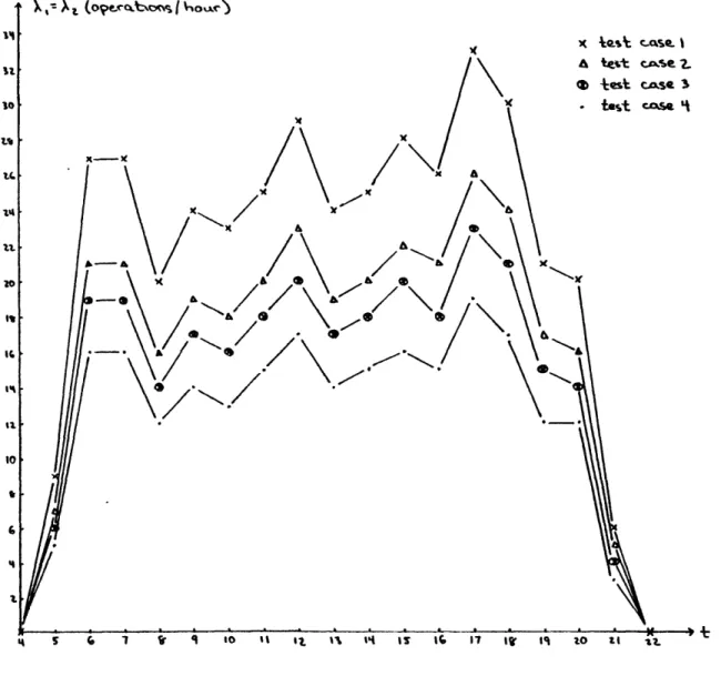
The average demand profile (in this case we assume that X (t) = X₂(t)) was obtained by connecting hourly data points for a hypothetical demand

profile in a piecewise linear manner. This profile appears as case 1 in Figure 3-1. Since demand for runway use in the early hours of the morning is negligible, we initialize the solution of the system equations

by assuming that at 4 AM the system is empty with probability 1.

Notice that for this particular system (p, = P2 P X1(t) + X2(t) =

2X1(t) = X(t), alternating priority for the two-.queue model), if the

queues have infinite capacity the single- and two-queue models should yield identical first moments for quantities such as the number of custo-mers in the system, the number of custocusto-mers in queue, and the delay faced by any aircraft. However, if finite queue sizes are imposed care must be taken when making these comparisons.

Suppose that we specify the maximum number of aircraft in the single-queue system to be 2M with M equal to the maximum number of each type allowed in the two-queue case (i.e., Nl = N2 = M). If M is too small, with a nonnegligible probability, aircraft will arrive to find a full

queue and thus will be turned away. If this situation occurs, although the maximum number of aircraft allowed in each of the models is identical, more aircraft will be lost (i.e., turned away) in the two-queue system

-28-Figure 3-1: Demand Profiles for Test Cases 1-4

than in the single-queue system. Thus, the expected number of aircraft in the system will be higher in the single-queue case.

We solved the single-queue and the basic two-queue models, with M = 15, under several levels of the "demand-to-capacity ratio" (p) - the measure of runway utilization. This ratio is defined to be the peak hour demand divided by the peak hour capacity. For the two-queue model:

peak hour demand = _{[X (t) + A2(t) peak hour}

and

peak hour capacity

=A

(t)

+

(

11. 2 ( peak hour

+

X

1

+

(tJpeak

hour

_(3.1)

This peak hour capacity is the sum of the average service rate of each type of aircraft weighted by the probability that that type of aircraft will be in service at the hour of peak demand. In the single-queue model

X(t) = X₁(t) + X2 (t), so

peak hour demand

[(t)p

peak hour and, as the average service rates are time-independent,

peak hour capacity = p.

All of the test cases used pi = p2 = P = 58 operations/hour, with the de-mand profile of case 1 scaled appropriately to yield the specified dede-mand-

demand-to-capacity ratio. The profiles for the two-queue model, p = 1.14, .9, .8, and .66, appear as cases 1 - 4 respectively in Figure 3-1.

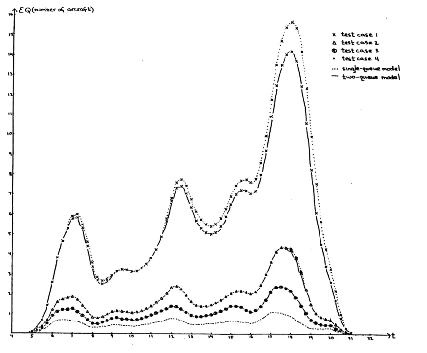
The expected number of aircraft in queue for each of these cases is shown in Figure 3-2 as a function of time. For p equal to .66 and .8,

E Q (ner oA awk tr9) x . .. a 4.w es - - ter.#

II

Wit'

-/

-..

Figure 3-2: _{Expected Number of Aircraft in Queue for Test Cases 1-4}

tese

I

the two models are indistinguishable. For the other two cases, at peri-ods of high demand, the number of aircraft arriving to a full queue was nonnegligible and, as expected, a greater number of planes were lost in the two-queue system. This difference is evident in the lower expected number in queue found in the two-queue case.

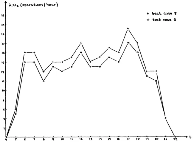
We studied two additional cases with X (t) = 2(t) and alternating

priority, but these examples used pi = 40 and p 2 = 60 operations/hour. Since X(t) = X₁(t) + x2(t) = 2 X1(t), to have the same demand-to-capacity

ratio in both the single- and two-queue models p was set equal to the peak hour capacity in this two-queue model, or (using equation (3.1))

p = 40 (1/2) + 60 (1/2) = 50 operations/hour.

The demand profiles for p = .9 and p = .8 appear as cases 5 and 6 in Figure 3-3.

Due to the nonlinear relationship between the average service rate and expected queue length, even if the queue capacities are infinite the single-queue and the two-queue models are no longer equivalent. Although in the long run we expect an equal number of each type of aircraft in ser-vice, the queue buildup during a lengthier (as compared to the single-queue system) type 1 service is not balanced by that of the shorter type 2 service and the two-queue system should, on average, have a greater number of aircraft in queue.

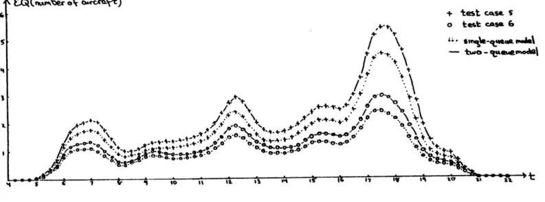
This is in fact the behavior illustrated in Figure 3-4 which shows the expected number of aircraft in queue for the single-queue and two-queue models, test cases 5 and 6. These runs used M = 15, a level high enough

to prevent the probability of an aircraft being turned away from becoming significant. Thus, the queue size is effectively infinite.

-32-AI,. (opecatons J VOwe')

!. .+ --++*,.+r e- +-. ,'..e- -~e4 ^'* -*.-.--o..e -.

*....Q +- .

-++'

.a

e&

I...-

-34-For the next test, we ran the basic model, under strict type 1 priority, for comparison with an existing M(t)/M/l simulation model. Comparing this case with the single-queue,analytical model would not be meaningful: when demands for landing and takeoff are the same, the single-queue model can be used to approximate a two-queue system with alternating priority, but it does not have the flexibility to take other priority schemes into account.

For these runs, the two-queue model used the demand profile of

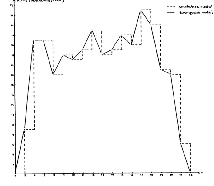
test case 1 and a maximum system size of 6 type 1 and 40 type 2 aircraft. The simulation, on the other hand, used a piecewise constant average demand which appears in Figure 3-5 with the piecewise linear profile of test case 1. Because of the differences in these two demand profiles we can not make exact comparisons between the models. In both models P1

and p2 were set at 58 operations/hour.

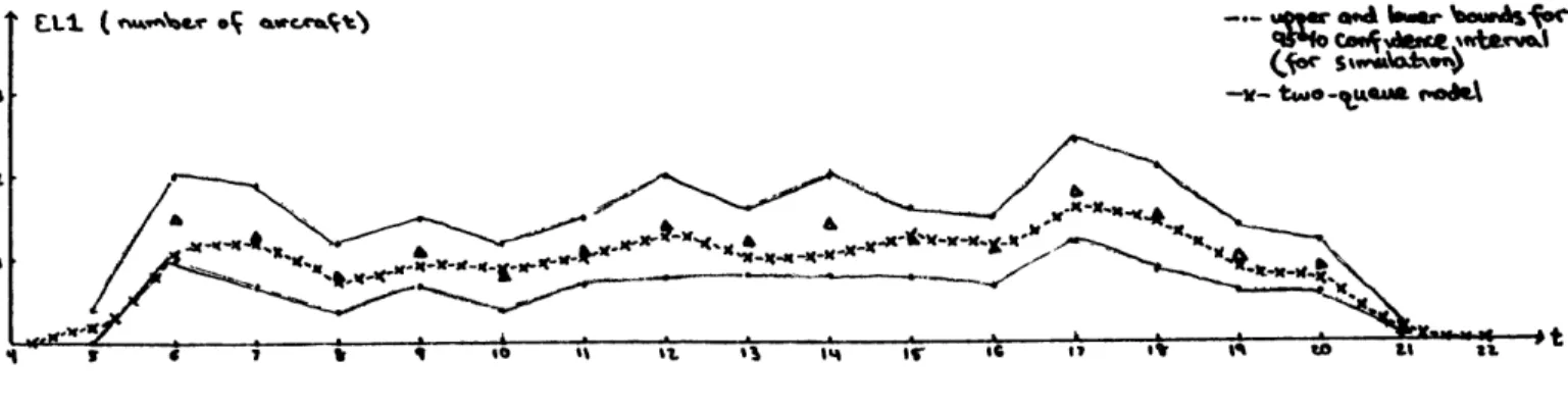
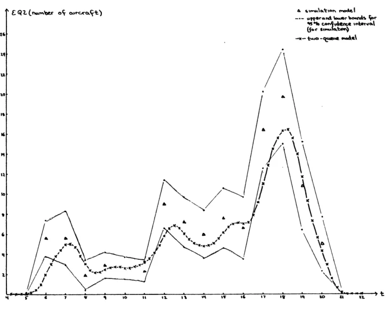
As a function of time, Figure 3-6 exhibits the expected number of type 1 aircraft in the system and Figure 3-7 shows the expected number of type 2 aircraft in queue for these two models. As can be seen from these figures, except for a few points in Figure 3-7, values from the two-queue model lie within the 95% confidence interval of the simula-tion. The disagreements can be explained by the differences in the de-mand profiles under the two models.

3.2 Using the Extended Model

To study the two-queue models in more depth, we return to a more accurate representation of behavior at the hypothetical airport. In

- - - siAot mode. -- two-*tqueA moe\

--I

\

Figure 3-5: Demand Profiles for Simulation and Two-Queue Models

A,--N.(.o eI-ons 5e

ELI *vAr ar %aws-J V tW~bjd*4 ta't

A

~

1 o i ' 9i 6 I t 14 It ILI It

v 1 10 II II. Iq to U Iu.

-38-Section 3.1 we selected p= = 58 operations/hour as appropriate average service rates only when aircraft of both types are awaiting service,

i.e., when successive aircraft are served on different runways. A more realistic picture of this intersecting runway situation can be obtained through use of the extended two-queue model under alternating priority with the following average service rates:

pl = ll = 29 operations/hour p20 22 = 55 operations/hour

p12 21 = 58 operations/hour.

These rates indicate that a stream of landings, allowed to use only one runway, will be served at an average rate of 29 operations/hour, and similarly, a stream of departures, using only the other runway, will have an average service rate of 55 operations/hour. As explained previously, when successive aircraft are of different types, the intersecting runway configuration handles aircraft in the same manner as a single runway on which aircraft of each type are served with an average rate of 58 operations/ hour. Thus the above values are appropriate for pl2 and p21'

In Figure 3-8 we show the expected number of aircraft in each queue for the extended model with the above service rates and the basic model with pl = P2 = 58 operations/hour To reduce computer costs, the less heavy demand profile of test case 2 (in Figure 3-1) was used. This allowed the system size, and thus the number of state equations, to be kept at a

-% %

* 81

-40-The final set of experimental results comes from the extended two-queue model of our hypothetical airport as just described. We once again used the demand profile of test case 2 and ran all four priority schemes introduced in Section 2.1.2. Figures 3-9 and 3-10 show the expected number of type 1 and type 2 aircraft in the system, respectively, under each of these schemes.

To interpret these resultsit is important to keep in mind the particular runway situation under consideration. Recall that, to model this two runway system using a single-server queueing model, the average service rates were chosen to specify that in a landing-takeoff-landing sequence the takeoff is inserted without interrupting the landing stream. Because of this, if alternating priority rules are in use, the number of type 1 aircraft in the system is not affected by the occurrence of take-offs. Thus, if we model the same airport situation but under strict type 1 priority rules, the expected number of aircraft of type 1 should be identical to that under alternating priority but the expected number of type 2 aircraft should be substantially larger. Under the strict type 1/alternating scheme, since takeoffs will not affect the landing stream under either strict type 1 or alternating priority rules, once again the expected number of type 1 aircraft in the system should be unchanged. As no departures will be allowed to begin during busy periods until the number of type 2 aircraft in the system is greater than the threshold

value, we anticipate the expected number of type 2 aircraft to lie be-tween those under alternating and strict type 1 priorities. For the strict type 1/strict type 2 scheme, whenever the threshold is exceeded,

-

h

v strt tpi ..

E.L % (nadoei oi % or~e..:)- **

eo stewt.t a./ t e t e .

a ztnect teWe i/cternet, x-I6 %/ X

.

I

o

~

/k

w&t

no type 1 aircraft will be allowed to begin service causing type 1 craft to accumulate rapidly. Thus, the expected number of type 1 air-craft in the system should exceed that under all of the other schemes, particularly at times of high demand. The expected number of type 2 aircraft in the system under strict type 1/strict type 2 priority should lie below the values under strict type 1 priority but the extent of this difference depends on the value of the threshold. The higher the thres-hold value, the closer the behavior under either thresthres-hold scheme will approach to that under strict type 1 priority rules. It is important to note that these results apply strictly, only when the queue capacities are effectively infinite.

In our tests, we specified system capacity to be a maximum of 13 aircraft of each type for all priority schemes except strict type 1. The threshold value (MCUT) was set at 3. In the alternating and strict type 1/alternating models, the probability that either queue becomes saturated turned out to be negligible at all hours of the day and hence the queue capacities were effectively infinite. As can be seen in Figures 3-9 and 3-10, behavior under these two schemes is as anticipated.

Under strict type 1/strict type 2 priority, at the peak period of the day a significant number of type 1 aircraft were lost. Thus, the values in Figure 3-9 are lower than anticipated.

For strict type 1 priority, we allowed a maximum of 5 type 1 and 30 type 2 aircraft in the system - lengths which caused a large number of aircraft to be lost (during the peak hours of the day the probability

-44-is full was about 20%). The aircraft turned away do not return to be served later, so the system is processing fewer total aircraft and thus the expected number of each type in the system should be consistently lower than anticipated - particularly at hours of peak demand. This is the behavior apparent in Figures 3-9 and 3-10 with the underestimate in the number of type 1 aircraft in the system particularly noticeable.

4. Expected Delay

Up to this point, statistics such as the expected queue lengths or expected number of aircraft of each type in the system have been used to indicate the relative system efficiency among different priority schemes. A measure which is usually of greater interest is the expected time delay faced by an aircraft entering the system at any time. Unfortunately, this is a very difficult quantity to determine for time-dependent, two-queue systems under priority schemes and a topic to which little research has been directed.

The quantity we are seeking is the expected time until a "virtual" aircraft entering the system at time T begins service. A "virtual" air-craft is one whose presence doesn't affect the system in any way.

In the remainder of this section we derive formulae for the expect-ed delay under two of the four priority schemes - alternating and strict type 1. The expected delay under the other two schemes, those involving a threshold, is an open research topic at this time. One observation is that the expected delay faced by a virtual aircraft of either type will be bounded from above and below by the expected delays to that type of aircraft under the strict type 1 and strict type 2 priority rules.

4.1 Alternating Priority

By assuming that there are aircraft of both types in the system at all times, we can obtain an estimate of the expected delay under alter-nating priority. We consider first the basic two-queue model and then expand this result to apply to the extended model. We then exhibit

-46-experimental results for test cases 2, 3 and 4 (of Section 3.1) compar-ing the expected delay under the scompar-ingle-queue and basic two-queue model under this scheme

Assume a virtual aircraft enters the system at time T and finds the system in state (I,J,l) 2 < I < Nl, 2 < J < N2 (i.e., queue 2 is nonempty

and neither queue is full). If the virtual aircraft is of type 1, it must wait for I-1 type 1 and I-1 type 2 service completions before it can

be-gin service. If the virtual aircraft is of type 2 it must wait for J type 1 and J-1 type 2 service completions. Similarly, if the system is in state (I,J,2) at time T, a type 1 virtual aircraft must wait for I-1 type 1 and I type 2 aircraft to be served while a type 2 virtual aircraft will wait for J-1 services of each type.

Since the arrival processes are independent and Poisson, at time T the probability that the arriving virtual aircraft at time T is of type 1 is

A(T) X1(T) + X2(T)

while the probability it is of type 2 is the complement of this quantity. For the basic model the service times have means of 1/p and 1/p2 for type 1 and type 2 aircraft respectively.

Under the assumption mentioned above, and suppressing the time de-pendence, the expected delay in hours, W, faced by a virtual aircraft entering the system at time T is

W = I (- + - )ELl + -]PROB2 +

(-

A+ X2 1 1 2

2 (il P2 i2 2

+

(-

+

-

)EL2]PROB2 +

(-

+

- )EL2 + -1PROBl

(4.1)

1i +2 11 P2 (1 P2 P11

When using the extended model p11 must be replaced by 1112 and p2 by p21' Without the assumption that aircraft of each type are always present in the system, formulae for the expected wait can be obtained by consider-ing many special cases individually. A general formula, however, has not yet been derived. We have thus used the above expression, (4.1), to

approximate the expected delay at all times for the test cases discussed below.

Two observations are in order, in this respect: first, due to the assumption that there is always a supply of each type of aircraft await-ing service, this analysis (usawait-ing expression (4.1)) should overestimate the expected wait. Second, we have exploited the no-memory property of Poisson processes: the additional amount of time (from time T) that the aircraft in service at time T will require to complete its service does not depend upon the time at which the service began.

Using expression (4.1), we calculated the expected delay in the basic two-queue model for each of test cases 2, 3 and 4 of Section 3.1. These de-lays, along with the corresponding expected delay in the single-queue mod-el, appear in Figure 4-1.

Recall that for these test cases the single-queue and two-queue sys-tem under alternating priority must have identical expected waiting times.

-48-a stcs.. e es e~..as 2 - ) m f Im al \6,4-a a. g T e i 60 a Aati t a 45 *6 Ar 1 % a 1 3 A 01 A Xa a'.

~

Figure 4-1: Expected Delay Under Alternating Priority for Three Levels of Runway Utilization

In the single-queue model, the expected delay can be determined exactly. Thus, we would expect expression (4.1) (an overestimate) to yield values above those given by the single-queue model. This behavior is apparent

in all three of the test cases. The performance of our approximation, however, for the most part seems to be quite satisfactory.

4.2 Strict Type 1 Priority

If landing aircraft are allowed absolute priority, we can derive exact expressions for the expected delay in the basic two-queue runway model by considering each type of virtual aircraft separately. In this

section we derive these expressions and apply them to test case 1 of Section 3.1.

Consider first a virtual aircraft of type 1 which enters the basic system at time T. This aircraft must wait for the plane currently in

service and those ahead of it in queue 1 to complete service before it will be allowed to land. Thus, its expected wait, Wl, is given by

=1 1 1

W1 = - PROB1 + - PROB2 + - EQ1 (4.2)

P_{1 P2 1}

(as usual, time dependence has been suppressed).

For the extended model the expression is slightly more complicated as the service time of the aircraft in service at time T depends on the type of the previous plane. If we define