Detecting information flow direction in multivariate linear and nonlinear models

(1)

HAL Id: inserm-00759802

https://www.hal.inserm.fr/inserm-00759802

Submitted on 4 Jan 2013

HAL is a multi-disciplinary open access archive for the deposit and dissemination of sci-entific research documents, whether they are pub-lished or not. The documents may come from teaching and research institutions in France or abroad, or from public or private research centers.

L’archive ouverte pluridisciplinaire HAL, est destinée au dépôt et à la diffusion de documents scientifiques de niveau recherche, publiés ou non, émanant des établissements d’enseignement et de recherche français ou étrangers, des laboratoires publics ou privés.

Detecting information flow direction in multivariate

linear and nonlinear models

Chunfeng Yang, Régine Le Bouquin-Jeannès, Gérard Faucon, Huazhong Shu

To cite this version:

Chunfeng Yang, Régine Le Bouquin-Jeannès, Gérard Faucon, Huazhong Shu. Detecting information flow direction in multivariate linear and nonlinear models. Signal Processing, Elsevier, 2013, 93 (1), pp.304-312. �10.1016/j.sigpro.2012.05.018�. �inserm-00759802�

(2)

Detecting information flow direction in multivariate linear and nonlinear models

Chunfeng Yanga, b, d_{(EURASIP Member), Régine Le Bouquin Jeannès}a, b, d_{*, Gérard Faucon}a, b, d_{, Huazhong Shu}c, d a_{U642, INSERM, F-35000, Rennes, France}

b_{LTSI, Université de Rennes 1, F-35000, Rennes, France}

c_{LIST, School of Computer Science and Engineering, Southeast University, 210096, Nanjing, China} d_{Centre de Recherche en Information Biomédicale Sino-Français (CRIBs)}

*Corresponding author: Régine Le Bouquin Jeannès (EURASIP Member) E-mail: [email protected]

Postal address: LTSI, Campus de Beaulieu, Bât 22, Université de Rennes 1, 35042, Rennes Cedex, France Tel: 33-2 23236220; Fax: 33-2 23236917

ABSTRACT: In this paper we present an approach to analyze the direction of information flow between time series

involv-ing bidirectional relations. The intuitive idea comes from a first study dedicated to the so-called phase slope index, which is a measure originally developed to detect unidirectional relations and is based on the complex coherence function. In order to detect bidirectional flows, we propose two new causality indices supplying the previous index with two other functions, the directed coherence function and the directed transfer function. Moreover, to cope with the inability of the approaches based on coherence (ordinary or directed) or on directed transfer function to distinguish between direct and indirect relations, we propose another causality index based on the partial directed coherence to identify only direct relations. Experimental results show that some challenges have promising solutions through the use of this new indicator dealing with both linear and non-linear multivariate models.

Keywords: Effective connectivity; causal relations; partial directed coherence; information flow; multivariate time series.

1. Introduction

In neuroscience, investigating activated cortical networks, in particular detecting direct interactions (directional ana-tomical links physiologically activated) between different cortical sites, helps in understanding brain functioning. Over the last decade, a number of measures have been considered to deal with causal dependency in multiple areas, such as physics, economics, chaotic systems and more particularly, effective connectivity in neurophysiology [2, 5, 8, 12, 14-18]. Recently, a Phase Slope Index (PSI) was proposed by Nolte [11] to detect information flow in unidirectional propagation graphs. The idea behind this measure is that the slope of the cross-spectrum phase between two different source activities depends on the time needed for the information flow between those areas and on the corresponding direction. This method, based on the linear phase between two signals, estimates the direction by computing the slope of the phase of the ordinary coherence

(3)

function. Now, when two time series may display direct or indirect relations, PSI based on the ordinary coherence function fails to distinguish between these two types of relations. As a matter of fact, when a third channel accounts for the linear re-lation between two other signals under scrutiny, the amplitude of the coherence function between these two signals is one (as it is when there is a direct linear relation between these signals). To deal with this issue, we recently proposed to replace or-dinary coherence with partial coherence [20]. As a matter of fact, let us consider the following simple scenario where signals

 

1

x t , x₂

 

t and x₃

 

t are given by:

 





 





 









 

1 1 1 2 1 2 3 2 1 3 0.9 1 0.5 1 0.8 2  2      _{ } _{ }   _ _ _ _ _  x t x t w t x t x t w t x t x t x t w t (1)

where w t_i

 



i1,2,3



are white Gaussian noises and the parameter  is introduced so as to possibly consider indirect (0) or direct ( 0.7) relations between the two time series x t₁

 

and x₃

 

t . In this example, if we compute the PSI based on the ordinary coherence [11], we find comparable values whatever  (for  0, PSI1.35, and for  0.7,

1.33 

PSI ), whereas results are very different when PSI is computed from the partial coherence (for  0, PSI0.01 whereas for  0.7, PSI0.95) which concludes to the success of the second indicator in detecting direct relations.

However, just like ordinary coherence, since the partial coherence function between two signals only carries a single direc-tion's information (given by the phase itself and its opposite value), it leads to a symmetric indicator and, consequently, is unable to detect bidirectional flows. As a matter of fact, if we consider a second scenario operating on the following three signals:

 





 









 





 

1 1 1 2 1 3 2 3 2 3 0.9 1 0.5 1 0.6 2 0.8 2      _{ } _{ } _ _   _ _ _  x t x t w t x t x t x t w t x t x t w t . (2)

In this example, a bidirectional relation exists between the two time series x₂

 

t and x₃

 

t . Computing the PSI from

 

2

x t to x3

 

t using coherence (resp. partial coherence) leads to a value close to 1.7 (resp. 0.7) whereas the PSI from

 

3

x t to x2

 

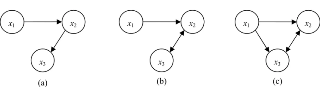
t returns the opposite value, i.e. -1.7 (resp. -0.7), so that it becomes impossible to detect bidirectional flows.

So, the aim of the present work is to mitigate the two previous issues. On the one hand, we investigate new causality indices (CI) to detect and differentiate unidirectional and bidirectional relations between multivariate time series (Fig. 1(a) and 1(b)): the first one is a new CI based on the directed coherence (DCOH) function [13] when considering pairwise analysis (i.e. only two observations are considered at the same time) and the second one is based on the directed transfer function (DTF) [9, 20] when considering multivariate analysis (i.e. joint analysis of more than two signals). On the other hand, to meet potential direct and indirect relations in bidirectional situations (Fig. 1(a) and 1(c)), we recommend to introduce partial directed co-herence (PDC) [3] in a new indicator. Until now, only the amplitudes of these different transfer functions have been

(4)

consid-ered in the literature to estimate the so-called functional connectivity between structures in the frequency domain. Such ap-proaches obviously failed in differentiating even quite simple scenarios, e.g. when two investigated observations only con-sisted of different time shifted versions of a third observation. In this paper, the three proposed causality indices are detailed theoretically in the next section. Linear and nonlinear time series are considered in a third section to test these indices and compare their performance before drawing some conclusions.

2. Methods and materials

Phase slope index (PSI) is a method to evaluate unidirectional information flows in pairs of signals [11]. After reviewing its concept and pointing out its theoretical limitations, we develop three new causality indices respectively based on DCOH, DTF and PDC.

2.1. Phase slope index

The PSI basic hypothesis relies on the exploitation of the phase monotony between signals which appears when the fre-quency components of one signal precede temporally those of another signal [11]. PSI is defined in order to summarize in-formation on the slope of the phase of the cross-spectrum between two time series x_m

 

t and x_n

 

t , t1,2,...,T , where

T is the signal length. The theoretical idea of this index is to properly represent relative time delays between spectral com-ponents of the two signals x_m and x_n only in the frequency bands leading to a significant value of the coherence function. To justify the formula introduced by Nolte to define his index, we consider the functional

 

_{ }

2 , m n mn f C f df f     



(3)

where C_mn

 

f S_mn

 

f / S_mm

 

f S_nn

 

f is the ordinary coherence function between signals x_m and x_n, with

( ) ( ) exp( ( ))

mn mn

C f C f i f and where the phase slope 

 



f

f , when it is constant, corresponds to a pure delay. Clearly, the squared magnitude of the coherence, C_mn

 

f 2, provides weighting the phase slope and, consequently, decreases its

impact when it is low. Hence, this functional is sensitive to both phase slope and coherence magnitude. As explained below the following expression

 









Im



_  

d mn mn f

f F C f C f (4)

is a numerical approximation of _{m n}_, which corresponds to the Phase slope index defined in [11] and is noted PSI_mn.

 

Im  denotes the imaginary part and the asterisk, the conjugate value; F is a discrete set of frequencies over which the _d

index is computed and which can be chosen by the experimenter according to some knowledge on the signals' characteristics. For example, if it is known that the signals are band limited, F can be reduced to only some critical frequencies. Similarly, _d

(5)

is given by: F_d 



0,1/ ,...,1 / 2N _f



where _f 1/N (in this case the frequential step-size _f corresponds to the frequency resolution 1/ N). The auto-spectral density functions S_mm

 

f and S_nn

 

f are the Fourier transforms of the auto-correlation of the signals x_m

 

t and x_n

 

t respectively, the cross-spectral density function S_mn

 

f is the Fourier transform of the cross-correlation between signals x_m

 

t and x_n

 

t defined by E x_ _m

  

t x*_n t



_, where E

 

 is the expectation operator and  is a time displacement. With C_mn( )f  C_mn( ) exp( ( ))f i f , we can write





PSI_mn



_{f F}_ sin (f _f)( )f C_mn( )f C_mn(f _f) , which can be approximated, for a sufficiently small _f , by





2

 

2 PSI _ (  )( ) ( ) _  





  i d mn _f _F i f i mn i _{f F} mn f f f C f C f df

f where the second term corresponds to a Rie-mann sum which is based on the assumption that the frequencies in F_d are regularly spaced with _f spacing and

ap-proximates the continuous sum (third term) on a continuous range F. The sign of PSI indicates the flow direction and its magnitude increases along with the delay and the coherence module. Clearly, this index (i) only works in situations of unidi-rectional connections, and (ii) cannot discriminate between direct and indirect relations. Following our notations, a positive value of PSI_mn means that the signal x_n is a delayed version of x_m. As it is well known, the linearity of the phase cor-responds to a pure delay between signals x_m and x_n. When one signal contributes to the second with multiple, different delays, the phase becomes nonlinear (the slope is no longer a constant). Nevertheless, to deal with a more general situation, we extend this idea to other coupling based functions as the phase is monotonic to propose novel causality indices, noted CI hereafter. While ordinary coherence focuses on mutual interaction of the structures themselves, directed coherence as well as directed transfer function refer more to the concept of Granger causality. This concept stipulates that a time series x t_i

 

causes another series x_j

 

t if the knowledge of x t_i

 

's past significantly improves the prediction of x_j

 

t . In this sense, only past samples are considered in improving prediction. Consequently, unlike ordinary coherence, directed coherence and directed transfer function are asymmetric quantities.

2.2. Causality index using directed coherence

The concept of directed coherence was first developed by Saito and Harashima [13] to jointly analyze information pro-duction in two time series, each having its proper white noise source, which can be seen as a local innovation, as well as a common source, seen as an external innovation. This can be represented with a bivariate autoregressive (AR) model for the production of signals. While coherence measures the degree of linear correlation as a total, the "directed coherences" can be seen as "correlations with direction" between the two observed signals expressed in the frequency domain and, interestingly, be regarded as two contributing weighted factors in the expression of the global coherence. Given these two observations (outputs of the system), these coherences describe the connection between the first (resp. second) noise input and the second

(6)

(resp. first) output of the system.

To formulate this problem of direction of correlating influences, Saito and Harashima considered a bivariate autoregres-sive process of order p including a common noise source w₃

 

t as follows:

 





 

1 11 13 1 11 12 1 3 23 22 2 1 21 22 2 2 0 -0 -        _    _        _ _          



p k w t b b x t k k x t k w t b b x t k k x t k w t (5)

where variables b_mn, m

 

1, 2 , n



1, 2,3



, are weight factors, w_j

 

t , j1, 2,3 are independent zero mean white Gaussian noises of unit variance. In the frequency domain, we have the spectral equivalent model:

 

1 2 2 1 11 12 1 1 11 13 1 3 2 2 ₂₃ ₂₂ 2 ₂₁ ₂₂ 1 1 2 1 11 13 11 12 3 23 22 21 22 2 1 ₀ 0 1 0 0                     _ _   __ _      _ _{ }      _   _ _ _         _ _     



p i fk p i fk k k p i fk p i fk k k dW f k e k e _b _b dX f dW f b b dX f _{k e} _{k e} dW f dW f b b A f A f dW f b b A f A f dW f   (6)

where dX1

 

f and dX2

 

f are the infinitesimal random spectral components [4] of the second order stochastic signals

 

1

x t and x₂

 

t , dW_j

 

f are those of the input noises w_j

 

t , j1, 2,3. Then, we introduce the matrix H f such

 

as:

 

11

 

_{ }

13

 

_{ }

12

 

_{ }

11

_{ }

 

12

_{ }

 

11 13 23 22 21 23 22 21 22 0 0                 b b H f H f H f A f A f H f b b H f H f H f A f A f . (7)

The DCOH estimate of the linear feedback from the innovation process w_m

 

t corresponding to the observation

 

m

x t to the observed signal x_n

 

t , with m n

 

1,2 , is

 

2 1,2,3 



 nm mn nj j H f DCOH f H f . (8)

Following the previous idea on PSI, we defined a causality index, named CI-DCOH, as follows:

 









CI_mn-DCOH Im



_{f F}_ DCOH_mn f DCOH_mn f _f . (9)

Contrary to the PSI, this index is asymmetric allowing the detection of bidirectional flows. It is no longer relative to the slope of the phase between the observations themselves but to those between the noise sources w_m( )t and the signals

 

n

x t , with m n

 

1, 2 .

2.3. Causality index using directed transfer function

Following the concept of directed coherence, the directed transfer function (DTF) was introduced by Kamiński and Bli-nowska [9] to deal with a number of observations greater than two. In this case, contrary to the previous situation, no hidden common noise source is considered, and each observation can be viewed as produced by its own innovation sequence line-arly combined with delayed versions of all observations. In the same manner as previously, directed transfer function from the i-th input to the j-th output of the system can be derived. Let it be indicated that both estimators are normalized with

(7)

respect to the structure that receives the signal. So, in the framework of multivariate observations, we extend the aforemen-tioned concept of causality index to DTF (instead of DCOH). Let x x₁, ₂, , x_Q be Q zero mean signals whose dis-crete-time observations are noted x t1( ), ( ),..., ( )x t2 xQ t . Suppose a multivariate AR model of order p to represent the

observations. Using the lag operator L



Lx_m

 

t x_m



t1



, m1, 2,...,Q



, we write

 

11 12 1 1 1 1 1 1 21 22 2 1 1 1 1 2 1 1 1 1 1 1                     _ _ _   _ _{ } _  _ _ _ _ _{ } _  _ _{ }_ _  _ _{ } _  _ _{ } _ _ _ _   



          p k p k p k Q k k k p k p k p k Q k k k Q Q p k p k p k Q Q QQ k k k k L k L k L x t w t k L k L k L x t w t k L k L k L . (10)

where w_m( )t are white Gaussian noises (innovations), and each regressor _mn

 

k , m n, 



1, 2,...,Q , evaluates the linear



interaction of x_n



tk on



w_m

 

t . Applying Fourier transform to the transfer functions matrix  in (10), we get the corresponding matrix D f :

 

11 12 1 21 22 2 1 2                       Q Q Q Q QQ D f D f D f D f D f D f D f D f D f D f (11)

where the components of the matrix D f are

 

2 1 2 1 1 , ,                 



p i fk mn k mn _p i fk mn k k e m n D f k e m n .

Defining the transfer matrix H f

 

as the inverse of the matrix D f

 

, we obtain

 

1 11 12 1 11 12 1 21 22 2 21 22 2 1 2 1 2              _ _{ } _                           Q Q Q Q Q Q QQ Q Q QQ H f H f H f D f D f D f H f H f H f D f D f D f H f H f H f H f D f D f D f . (12)

The Directed Transfer Function from channel m to channel n is defined by:

 

2 1 



 nm mn Q nm m H f DTF f H f (13)

where H_nm

 

f is the



n m,



element of the matrix H f

 

, corresponding to a normalized contribution of the input se-quence w_m

 

t onto the output signal x_n

 

t . In the same way as before, we defined a causality index based on DTF, noted CI-DTF, as follows:

 









CI_mn-DTF Im



_{f F}_ DTF_mn f DTF_mn f _f . (14)

(8)

Following the above developments, in [3] Baccalá and Sameshima contrasted partial directed coherence with directed coherence to show how partial directed coherence provides direct structural information for multivariate time signals, as par-tial coherence does compared to ordinary coherence in unidirectional flow models. So, given Q2 observations, the

par-tial directed coherence function describes the interaction between two of these observations when the influence due to all other Q2 time series is discounted. According to Eq. (11), the PDC from x_m to x_n conditionally to other Q2 signals can be written

 

† _  nm mn m m D f PDC f d f d f (15) where D_nm

 

f is the



n m,



element of D f

 

and d_m

 

f is the mth column of D f

 

. D_nm

 

f represents the

part of the past of x_m on the present signal x_n. The sign † denotes conjugate transpose. The arguments to define a PDC based causality index can be fully justified as we want to develop an average measure (i) to quantify the relative delays be-tween multiple signals and not only to qualify them as the PDC magnitude did, and (ii) to weight properly different fre-quency bands according to the strength of the direct coupling. Consequently, we propose to define here a PDC based causal-ity index measure, noted CI-PDC, by

 









CI_mn-PDC Im



_ _mn _mn _f

f FPDC f PDC f . (16)

If the only contribution of the signal x_m into the signal x_n is due to a pure delay, the phase of D_nm

 

f as well as the phase of PDC are linear, so that CI-PDC represents the slope of this phase, weighted by the magnitude of PDC.

2.5. Effect of deviation from linear model hypothesis

In some applications the model given in (10) is not the more realistic one and a non linear regression model (17) would be more suited

 





 





 





1 1 1 1 1,.., 1 ,.., , , ( ) , 1,.., ,.., ,                        _{ } _    Q Q d d d k i i k d d d Q Q Q g x x w t x t x t L x t i Q x t g x x w t (17)

where g i_i, 1,.., ,Q are non linear functions. The efficiency of a linear model (10) to detect non linear incidence from channels mM₁



1,..,Q



to channel n (from xd_m, mM₁, to x_n) then depends a priori on the ability of a

decompo-sition sum

 

,1 ,2 ,1 _ ,2 _ ,           n   n  d d n m n m n m M m M

g x t g x w t to approximate the function



₁,.., ,



 

Q d d n n g x x w t where





,1 ,2 1,.., , ,1 ,2  n n n n

M M Q M M ; g_n_,1 is a linear function and g_n_,2 is non linear. Only if the difference between

n

g and gn,1gn,2 is not too important, we can expect that the indices described above remain relevant. Otherwise, in

(9)

exam-ple on local linear approximations around reference points [6]. Nevertheless note that in this case the phase slope informa-tion could be less adapted, since it cannot capture phase relainforma-tion between two different frequencies.

3. Experimental results

The different approaches were tested on models simulating practical situations and, for all of them, spectral estimation was based on AR modeling which can improve the estimator and reduce its variance as indicated in [20]. For each model, simulations were carried out 500 times on 1024-point signals (corresponding to 4 s duration with a sampling rate equal to 256 Hz). We calculated N frequency points regularly spaced, with N512, and the frequential step-size _f was equal to 0.25 Hz. In our experiments, the AR coefficients and the order of the models were firstly estimated from the generated data by minimizing Akaike's information criterion (AIC) [1]. This was performed by using the functions lsqr and aic in MATLAB which, supposing Gaussian innovations, maximize a likelihood function through a least squares (LS) procedure [10] (chapter 16, section 16.4). Given these estimated parameters, we computed matrices H f

 

and D f

 

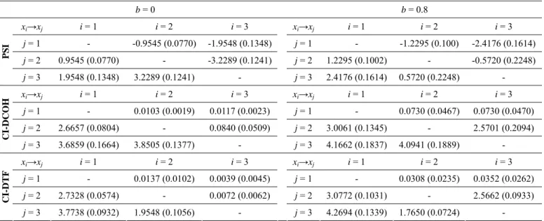
of Eqs. (7), (12) and (11) respectively by substitution of theoretical AR coefficients with the estimated ones. This procedure allows for obtaining CI-DCOH, CI-DTF and CI-PDC. Results are summarized in Tables 1 to 4, where the first value corresponds to the experimental mean of the indicator and the experimental standard deviation (sd) is in brackets.

3.1. Linear models

We start by analyzing the behavior of our estimators on signals exhibiting bidirectional propagation flows (model 1). Then, we test them on a model (model 2) displaying direct and indirect connections.

3.1.1. Model 1

For the first linear stochastic system, three signals were generated by the following equations

 









 









 





 

1 1 1 1 2 1 3 2 3 2 3 0.95 2 1 0.9025 2 0.5 1 3 0.8 2                _ _ _  x t x t x t w t x t x t bx t w t x t x t w t (18)

where w_j

 

t ,j1,2,3, are independent white Gaussian noises with zero means and unit variances, the parameter b was introduced to consider two patterns of causal interactions with unidirectional (b0; Fig. 1(a)) or bidirectional (b0.8; Fig.

1(b)) relations between signals x and 2 x . Means and standard deviations of PSI, CI-DCOH and CI-DTF were computed 3

and shown in Table 1.  Results on PSI

From Table 1, when there are only unidirectional (direct and/or indirect) information flows, i.e. b0, PSI12, PSI23 and PSI13 gave positive values indicating that x is a delayed version of 2 x , and 1 x some delayed version of 3 x and 2 x . 1

When there is a bidirectional information flow between x and ₂ x (i.e. ₃ b0.8), PSI necessarily fails in detecting the

(10)

unidirectional flows.

 Results on CI-DCOH

In Table 1, considering the case b0, when there is no information flow, i.e. from x to 2 x , or from 1 x to 3 x , or 1

from x to 3 x , the corresponding CI-DCOH remains close to zero. On the other hand, when unidirectional information 2

flows exists, i.e. from x to ₁ x , or from ₂ x to ₁ x , or from ₃ x to ₂ x , the corresponding CI-DCOH largely increases. ₃

Considering the case b0.8, the same conclusions hold. Moreover, in this case of bidirectional flow between x and ₂ x , ₃

CI-DCOH is also able to determine this particular propagation, so that it appears as a relevant indicator to detect unidirec-tional and bidirecunidirec-tional relations.

 Results on CI-DTF

For the case b0, the very low values of CI21-DTF, CI31-DTF and CI32-DTF are clearly justified as well as the great values of CI12-DTF, CI13-DTF and CI23-DTF due to only unidirectional flows. For the case b0.8, all unidirectional and bidirectional flows are also properly detected. Therefore, CI-DTF behaves well in all situations and proves efficient in draw-ing the real propagation graphs.

In a second step, we compare the performance of CI-DCOH and CI-DTF from Table 1. On the one hand, whatever the value of b , the values of CI-DCOH are greater than those given by CI-DTF for the flow from x to ₂ x . On the other ₃

hand, in the bidirectional situation (i.e. b0.8), the ratio CI -DTF/CI -DTF₃₂ ₂₃ is closer to 3/2 corresponding to the ratio of the delays between signals x and ₂ x . ₃

3.1.2. Model 2

For the second linear stochastic system we considered, the signal propagation situation was formalized as

 









 









 









 

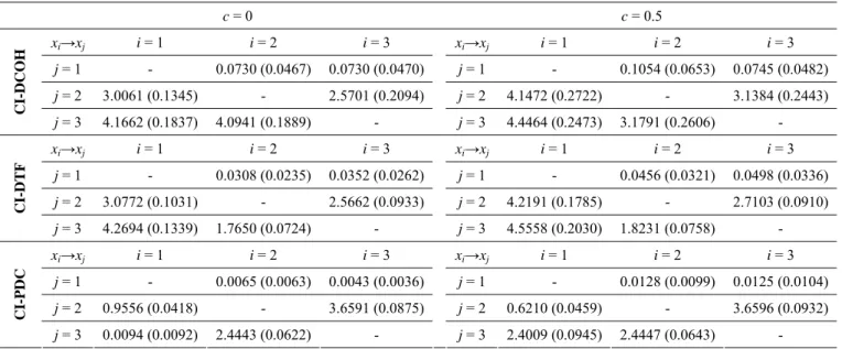
1 1 1 1 2 1 3 2 3 2 1 3 0.95 2 1 0.9025 2 0.5 1 0.8 3 0.8 2 4                _ _ _ _ _  x t x t x t w t x t x t x t w t x t x t cx t w t (19)

where w_j

 

t , j1,2,3, are independent white Gaussian noises with zero means and unit variances, and the parameter c was chosen to consider two patterns of interactions including indirect (c0; Fig. 1(b)) and direct (c0.5; Fig. 1(c))

rela-tionships from signal x to signal 1 x . In this system, a bidirectional flow was modeled between signals 3 x and 2 x . 3

Means and standard deviations of CI-DCOH, CI-DTF and CI-PDC are calculated and presented in Table 2.  Results on CI-DCOH

As already shown in Table 1, CI-DCOH allows for pointing out of unidirectional and bidirectional relations (see Table 2, either c0 or c0.5). On the other hand, when two different interactions exist from x to ₁ x , i.e. indirect (₃ c0) and

direct (c0.5, x connects to 1 x via two distinct pathways) interactions, CI3 13-DCOH reveals comparable values and, so, it becomes impossible to distinguish between direct and indirect interactions.

(11)

 Results on CI-DTF

As previously, we can conclude from Table 2 that CI-DTF succeeds in pointing out unidirectional and bidirectional rela-tions but fails in distinguishing direct and indirect relarela-tions like CI-DCOH. Nevertheless, even if CI-DTF cannot reveal the delays between signals in the bidirectional case, one can at least infer the value of the delays' ratio between x and 2 x (a 3

2-time delay from x to ₂ x and a 3-time delay from ₃ x to ₃ x ). As a matter of fact, the ratio ₂ CI -DTF/CI -DTF₃₂ ₂₃ is

always around 3/2 regardless if c0 or c0.5, whereas the ratio CI -DCOH/CI -DCOH₃₂ ₂₃ varies more (around 0.6

when c0 and 1.0 when c0.5).

 Results on CI-PDC

Like CI-DCOH and CI-DTF, from Table 2 CI-PDC succeeds in detecting unidirectional and bidirectional relations. Moreover, when there is only indirect flow from x to ₁ x (for 3 c0), CI13-PDC remains close to zero; and, when there is direct relation from x to 1 x (for 3 c0.5), CI13-PDC increases significantly. In this way, CI-PDC clearly con-trasts with CI-DCOH and CI-DTF, since these two quantities always display a non negligible value when tested from signal 1 to signal 3, whatever the value of c . Therefore, CI-PDC resolves the existence of direct and indirect connections between pairs of signals by distinguishing these kinds of connections.

Finally, for the bidirectional relation between x and ₂ x , the ratios ₃ CI -PDC/CI -PDC₃₂ ₂₃ are close to 3/2 regardless

if c0 or c0.5 like CI-DTF. Furthermore, the value of CI23-PDC (resp. CI32-PDC) is greater than the value of CI23-DTF (resp. CI32-DTF), which appears more justified corresponding to some smoothing of the noise influence.

3.2. Nonlinear models

To test the robustness of our estimators to nonlinearity, we first tested a nonlinear model (model 3) where the coupling be-tween signals is still linear. In a second step, the nonlinearity of the coupling is also taken into account (model 4).

3.2.1. Model 3

The first nonlinear stochastic system we investigated was as follows:

 









 









 









 









 









 

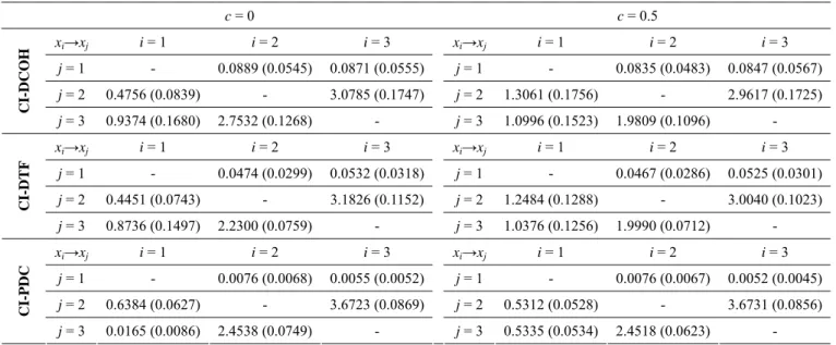
2 1 2 2 2 3 1 2 1 1 1 1 1 2 2 2 2 1 3 2 1 2 3 3 3 2 1 3 3.4 1 1 1 3.4 1 1 1 0.5 1 0.8 3 3.4 1 1 1 0.8 2 1        _ _ _ _ _   _ _ _ _ _ _{ } _{ }    _ _ _ _ _ _ _ _{ }  x t x t x t x t x t x t e w t x t x t x t e x t x t w t x t x t x t e x t cx t w t (20)

where w_j

 

t ,j1,2,3, are independent white Gaussian noises with zero means and unit variances, and the parameter c

was introduced to model direct or indirect interactions as in Eq. (19). Here we have

 

_ _

 

_{ }

 



 



 

2 __1,2,3 , 2  2,1 __1,3   2,2 _₂, 2     d d d m m m m m m

g x w t g x t g x w t , and so we can expect to detect the influences from

1

(12)

lin-ear methods according to

 

 

 

 

 



 



 

3 __1,2,3 , 3  3,1 __1,2   3,2 _₃, 3     d d d m m m m m m

g x w t g x t g x w t . Means and standard

de-viations of CI-DCOH, CI-DTF and CI-PDC are given in Table 3.  Results on CI-DCOH and CI-DTF

Means and standard deviations of CI-DCOH and CI-DTF highlighted the ability of these two indices to put forward uni-directional and biuni-directional interactions. As in the second linear model (see section 3.1.2, Eq. (19)), both CI-DCOH and CI-DTF could not differentiate between direct and indirect interactions from signal x1 to signal x3.

Comparing CI-DCOH and CI-DTF, if we consider the relations between x2 and x3, we first observe that CI-DTF

dis-plays greater values in the nonlinear model than in the linear one (model 2) unlike CI-DCOH. As in the linear case, this re-sult is explained by the signals' characteristics. Secondly, in this bidirectional case, CI-DTF is still representative of the rela-tive dependence that exists between x₂ and x₃: the ratio CI -DTF/CI -DTF₃₂ ₂₃ is around 3/2 regardless of the model (linear or nonlinear) and the pattern (indirect and direct interactions from x₁ to x₃).

 Results on CI-PDC

Results on CI-PDC reported in Table 3 lead to the same conclusions as those derived in the linear case (see section 3.1.2). CI-PDC acts as the most suitable and relevant indicator not only in detecting unidirectional and bidirectional relations but also in differentiating direct and indirect relations. For the bidirectional relation between x2 and x3, the ratios

32 23

CI -PDC/CI -PDC are also closer to 3/2 regardless of the value of c like CI-DTF. Moreover, CI23-PDC (resp. CI32-PDC) is also greater than CI23-DTF (resp. CI32-DTF) which is a worthwhile expected result.

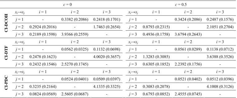
3.2.2. Model 4

The second nonlinear stochastic system with nonlinear coupling was generated by the equations

 









 









 









 









 









 

2 1 2 2 2 2 1 2 1 1 1 1 1 2 2 2 2 2 1 3 2 1 2 3 2 2 2 1 3 3.4 1 1 1 3.4 1 1 1 0.8 3 0.8 3 3.4 1 1 1 0.8 2 1        _ _ _ _ _   _ _ _ _ _ _{ } _{ }    _ _ _ _ _ _{ } _{ }  x t x t x t x t x t x t e w t x t x t x t e x t x t w t x t x t x t e x t cx t w t (21)

where w_j

 

t ,j1,2,3, are independent white Gaussian noises with zero means and unit variances, and the parameter c was introduced to model direct or indirect interactions as in Eq. (19). Here we have

 

_ _

 



 



 

2 __1,2,3 , 2  2,1 _₃  2,2 __1,2, 2     d d d m m m m m m

g x w t g x t g x w t , and we can expect to detect the influences from x₃ to x₂ with linear methods. Similarly for the third signal, we can expect to detect the influences from x₁ to x₃ with linear methods according to

 

 

 



 



 



 



 

3 __1,2,3 , 3  3,1 _₁  3,2 _₂, 3   d d d m m m m m m

g x w t g x t g x w t (according to the definition re-tained in section 2.5, all delayed versions of signal x₂ are included in the nonlinear function g_3,2). Note that, comparing with model 3, we introduced in model 4 a nonlinear coupling to test the influence of linearity versus nonlinearity of coupling. Means

(13)

and standard deviations of CI-DCOH, CI-DTF and CI-PDC are given in Table 4. Despite a global increase in the standard de-viation, the mean values of the different indicators are of the same order of magnitude as those shown in Table 3. Considering CI-DCOH, when comparing signals two by two, we note that this indicator is affected by the nonlinear coupling to detect cor-rectly the relations between x1 and x2, as well as between x1 and x3. On the other hand, the CI-DTF indicator allows

detecting unidirectional and bidirectional relations despite the introduction of this nonlinear coupling and CI-PDC still performs well in differentiating direct and indirect relations.

4. Discussion and conclusion

As shown in this study, the information flows among multivariable observations can display different patterns including unidirectional and/or bidirectional relations, direct and/or indirect relations. The original ordinary coherence based phase slope index only appears suitable to detect unidirectional flows when considering two time series. In this paper, we focus on information propagation between multi-site observations. The interest of the techniques we propose can be summarized as follows: (i) the introduction of directed coherence (DCOH) and directed transfer function (DTF) allows for dealing with uni-directional and biuni-directional relations; (ii) moreover, the introduction of partial directed coherence (PDC) allows for distin-guishing direct and indirect relations for unidirectional as well as bidirectional flow. In so far as we know, only amplitudes of DCOH, DTF and PDC have already been investigated to deal with the difficult issue of coupling between time series. In this contribution, both amplitudes and phases of these functions have been introduced to develop new causality indices that pear more relevant to flow propagation. Among the different techniques, the partial directed coherence function based ap-proach has an advantage over the others since it takes into account only the direct contribution of a signal x_m on another signal x_n to compute the corresponding phase slope. It behaves well in distinguishing direct and indirect relations either for unidirectional or bidirectional flows. Now, if CI-PDC seems to be the best technique to differentiate all patterns in the pro-posed linear and nonlinear multivariate autoregressive models, real biological patterns may be more complex (EEG, ECG, EMG, etc.), which support the proposal of these different indicators. Moreover, according to EEG models found in the lit-erature [7, 19], we can expect that in many practical cases the nonlinearities are sufficiently smooth, so that the indicators remain relevant. In the future, we plan to test them to characterize the underlying network organization of an epileptic sei-zure, in some difficult situation where time shifts between signals vary strongly in time. Clearly practical use of these indi-cators will imply the introduction of decision thresholds to reject the null hypothesis (no connectivity). Classically, as it is difficult to obtain theoretical distribution under independence, it will be necessary to obtain it empirically, for example using surrogate data. In such a situation, as in many other applications involving more than two or three channels, the computa-tional cost of linear AR identification and phase analysis is highly reduced compared to the case of non linear analysis, which can then be only considered to solve ambiguous cases. Finally, despite the basic idea behind the indices developed in this work, which can be viewed as detecting linear phase slopes associated with pure delay, this phase linearity does not need

(14)

to be verified to expect interesting results: only a monotonic phase variation with a significant mean slope is required. It is important to note that generally, when using DCOH and DTF, the phase linearity is not verified, due to the intrinsic defini-tion of such quantities. In the same manner, the PDC based index corresponds to linear phase only when there is a unique contribution (in terms of delay) of a first signal to a second. In a future work, we can also search for other choices of func-tions q and C_mn in (3), depending on the index property we want to emphasize. To conclude, it could be also interesting to extend phase analysis based on linear regression models to a higher order phase analysis based on polynomial regression models.

Acknowledgements

The authors thank Jean-Jacques Bellanger for fruitful discussions and the anonymous reviewers for comments on this manu-script.

References

[1] H. Akaike, Information theory and an extension of the maximum likelihood principle, vol. the Second International Sympo-sium on Information Theory, Budapest, Hungary, 1973, pp. 267-281.

[2] P. O. Amblard, O. J. J. Michel, On directed information theory and Granger causality graphs, Journal of Computational Neuroscience, 30 (2010) 7-16.

[3] L. A. Baccalá, K. Sameshima, Partial directed coherence: a new concept in neural structure determination, Biological Cy-bernetics, 84 (6) (2001) 463-474.

[4] P. J. Brockwell, R. A. Davis, Time series: theory and methods, second ed., Springer Verlag, 1991. [5] G. C. Carter, Coherence and time delay estimation, Proceedings of the IEEE, 75 (2) (2005) 236-255.

[6] Y. Chen, G. Rangarajan, J. Feng, M. Ding, Analyzing multiple nonlinear time series with extended Granger causality, Phys-ics Letters A, 324 (1) (2004) 26-35.

[7] K. J. Friston, L. Harrison, W. Penny, Dynamic causal modelling, Neuroimage, 19 (4) (2003) 1273-1302.

[8] C. W. J. Granger, Investigating causal relations by econometric models and cross-spectral methods, Econometrica, 37 (3) (1969) 424-438.

(15)

[9] M. J. Kamiński, K. J. Blinowska, A new method of the description of the information flow in the brain structures, Biological Cybernetics, 65 (3) (1991) 203-210.

[10] L. Ljung, System identification, Prentice-Hall, New Jersey, American, 1987.

[11] G. Nolte, A. Ziehe, V. V. Nikulin, A. Schlögl, N. Krämer, T. Brismar, K. R. Müller, Robustly estimating the flow direction of information in complex physical systems, Physical Review Letters, 100 (23) (2008) 234101.

[12] S. Sabesan, L. Good, K. Tsakalis, A. Spanias, D. Treiman, L. Iasemidis, Information flow and application to epileptogenic focus localization from intracranial EEG, IEEE transactions on neural systems and rehabilitation engineering: a publication of the IEEE Engineering in Medicine and Biology Society, 17 (No. 3) (2009) 244-253.

[13] Y. Saito, H. Harashima, Tracking of information within multichannel EEG record-causal analysis in EEG, El-sevier-North-Holland Biomedical Press, Amsterdam, 1981.

[14] A. Salazar, L. Vergara, R. Miralles, On including sequential dependence in ICA mixture models, Signal Processing, 90 (7) (2010) 2314-2318.

[15] S. Spasic, Surrogate data test for nonlinearity of the rat cerebellar electrocorticogram in the model of brain injury, Signal Processing, 90 (12) (2010) 3015-3025.

[16] K. E. Stephan, L. Kasper, L. M. Harrison, J. Daunizeau, H. E. M. den Ouden, M. Breakspear, K. J. Friston, Nonlinear dy-namic causal models for fMRI, NeuroImage, 42 (2) (2008) 649-662.

[17] B. Veeramani, K. Narayanan, A. Prasad, L. D. Iasemidis, A. S. Spanias, K. Tsakalis, Measuring the direction and the strength of coupling in nonlinear systems-a modeling approach in the state space, IEEE Signal Processing Letters 11 (7) (2004) 617-620.

[18] X. Wang, Y. Chen, S. L. Bressler, M. Ding, Granger causality between multiple interdependent neurobiological time series: Blockwise versus pairwise methods, International journal of neural systems, 17 (2) (2007) 71-78.

(16)

[19] F. Wendling, A. Hernandez, J. J. Bellanger, P. Chauvel, F. Bartolomei, Interictal to ictal transition in human temporal lobe epilepsy: insights from a computational model of intracerebral EEG, Journal of Clinical Neurophysiology, 22 (5) (2005) 343-356.

[20] C. Yang, R. Le Bouquin-Jeannès, G. Faucon, H. Shu, Extracting information on flow direction in multivariate time series, IEEE Signal Processing Letters, 18 (4) (2011) 251-254.

Fig. 1. Three patterns of causal interactions. (a) Connection from signal x1 to signal x3 is indirect and mediated by signal x2, and only unidirectional pathways exist. (b) Bidirectional flow exists between signals x2 and x3. (c) Both direct and indirect connec-tions exist from signal x1 to signal x3, and bidirectional flow exists between signals x2 and x3.

x1 x2 (a) x3 (c) x1 x2 x3 (b) x1 x2 x3

(17)

Table 1. Results on PSI, CI-DCOH and CI-DTF in Model 1 (Eq. (18)) b = 0 b = 0.8 xi→xj i = 1 i = 2 i = 3 xi→xj i = 1 i = 2 i = 3 j = 1 - -0.9545 (0.0770) -1.9548 (0.1348) j = 1 - -1.2295 (0.100) -2.4176 (0.1614) j = 2 0.9545 (0.0770) - -3.2289 (0.1241) j = 2 1.2295 (0.1002) - -0.5720 (0.2248) PS I j = 3 1.9548 (0.1348) 3.2289 (0.1241) - j = 3 2.4176 (0.1614) 0.5720 (0.2248) - xi→xj i = 1 i = 2 i = 3 xi→xj i = 1 i = 2 i = 3 j = 1 - 0.0103 (0.0019) 0.0117 (0.0023) j = 1 - 0.0730 (0.0467) 0.0730 (0.0470) j = 2 2.6657 (0.0804) - 0.0840 (0.0509) j = 2 3.0061 (0.1345) - 2.5701 (0.2094) CI-DCOH j = 3 3.6859 (0.1664) 3.8505 (0.1377) - j = 3 4.1662 (0.1837) 4.0941 (0.1889) - xi→xj i = 1 i = 2 i = 3 xi→xj i = 1 i = 2 i = 3 j = 1 - 0.0137 (0.0102) 0.0039 (0.0045) j = 1 - 0.0308 (0.0235) 0.0352 (0.0262) j = 2 2.7328 (0.0574) - 0.0072 (0.0062) j = 2 3.0772 (0.1031) - 2.5662 (0.0933) CI-DTF j = 3 3.7738 (0.0932) 1.9548 (0.1056) - j = 3 4.2694 (0.1339) 1.7650 (0.0724) -

(18)

Table 2. Results on CI-DCOH, CI-DTF and CI-PDC in Model 2 (Eq. (19)) c = 0 c = 0.5 xi→xj i = 1 i = 2 i = 3 xi→xj i = 1 i = 2 i = 3 j = 1 - 0.0730 (0.0467) 0.0730 (0.0470) j = 1 - 0.1054 (0.0653) 0.0745 (0.0482) j = 2 3.0061 (0.1345) - 2.5701 (0.2094) j = 2 4.1472 (0.2722) - 3.1384 (0.2443) CI-DCOH j = 3 4.1662 (0.1837) 4.0941 (0.1889) - j = 3 4.4464 (0.2473) 3.1791 (0.2606) - xi→xj i = 1 i = 2 i = 3 xi→xj i = 1 i = 2 i = 3 j = 1 - 0.0308 (0.0235) 0.0352 (0.0262) j = 1 - 0.0456 (0.0321) 0.0498 (0.0336) j = 2 3.0772 (0.1031) - 2.5662 (0.0933) j = 2 4.2191 (0.1785) - 2.7103 (0.0910) CI-DTF j = 3 4.2694 (0.1339) 1.7650 (0.0724) - j = 3 4.5558 (0.2030) 1.8231 (0.0758) - xi→xj i = 1 i = 2 i = 3 xi→xj i = 1 i = 2 i = 3 j = 1 - 0.0065 (0.0063) 0.0043 (0.0036) j = 1 - 0.0128 (0.0099) 0.0125 (0.0104) j = 2 0.9556 (0.0418) - 3.6591 (0.0875) j = 2 0.6210 (0.0459) - 3.6596 (0.0932) CI-PDC j = 3 0.0094 (0.0092) 2.4443 (0.0622) - j = 3 2.4009 (0.0945) 2.4447 (0.0643) -

(19)

(20)