HAL Id: hal-00295801
https://hal.archives-ouvertes.fr/hal-00295801
Submitted on 14 Dec 2005
HAL is a multi-disciplinary open access
archive for the deposit and dissemination of
sci-entific research documents, whether they are
pub-lished or not. The documents may come from
teaching and research institutions in France or
abroad, or from public or private research centers.
L’archive ouverte pluridisciplinaire HAL, est
destinée au dépôt et à la diffusion de documents
scientifiques de niveau recherche, publiés ou non,
émanant des établissements d’enseignement et de
recherche français ou étrangers, des laboratoires
publics ou privés.
retrieved from SCIAMACHY by WFM-DOAS: year
2003 initial data set
M. Buchwitz, R. de Beek, S. Noël, J. P. Burrows, H. Bovensmann, H. Bremer,
P. Bergamaschi, S. Körner, M. Heimann
To cite this version:
M. Buchwitz, R. de Beek, S. Noël, J. P. Burrows, H. Bovensmann, et al.. Carbon monoxide, methane
and carbon dioxide columns retrieved from SCIAMACHY by WFM-DOAS: year 2003 initial data
set. Atmospheric Chemistry and Physics, European Geosciences Union, 2005, 5 (12), pp.3313-3329.
�hal-00295801�
Atmos. Chem. Phys., 5, 3313–3329, 2005 www.atmos-chem-phys.org/acp/5/3313/ SRef-ID: 1680-7324/acp/2005-5-3313 European Geosciences Union
Atmospheric
Chemistry
and Physics
Carbon monoxide, methane and carbon dioxide columns retrieved
from SCIAMACHY by WFM-DOAS: year 2003 initial data set
M. Buchwitz1, R. de Beek1, S. No¨el1, J. P. Burrows1, H. Bovensmann1, H. Bremer1, P. Bergamaschi2, S. K¨orner3, and
M. Heimann3
1Institute of Environmental Physics (IUP), University of Bremen FB1, Bremen, Germany 2Institute for Environment and Sustainability, Joint Research Centre (EC-JRC-IES), Ispra, Italy 3Max Planck Institute for Biogeochemistry (MPI-BGC), Jena, Germany
Received: 27 January 2005 – Published in Atmos. Chem. Phys. Discuss.: 1 April 2005 Revised: 27 June 2005 – Accepted: 23 November 2005 – Published: 14 December 2005
Abstract. The near-infrared nadir spectra measured by
SCIAMACHY on-board ENVISAT contain information on the vertical columns of important atmospheric trace gases such as carbon monoxide (CO), methane (CH4), and
car-bon dioxide (CO2). The scientific algorithm WFM-DOAS
has been used to retrieve this information. For CH4 and
CO2also column averaged mixing ratios (XCH4and XCO2)
have been determined by simultaneous measurements of the dry air mass. All available spectra of the year 2003 have been processed. We describe the algorithm versions used to generate the data (v0.4; for methane also v0.41) and show comparisons of monthly averaged data over land with global measurements (CO from MOPITT) and models (for CH4and
CO2). We show that elevated concentrations of CO
result-ing from biomass burnresult-ing have been detected in reasonable agreement with MOPITT. The measured XCH4is enhanced
over India, south-east Asia, and central Africa in Septem-ber/October 2003 in line with model simulations, where they result from surface sources of methane such as rice fields and wetlands. The CO2measurements over the Northern
Hemi-sphere show the lowest mixing ratios around July in quali-tative agreement with model simulations indicating that the large scale pattern of CO2uptake by the growing vegetation
can be detected with SCIAMACHY. We also identified po-tential problems such as a too low inter-hemispheric gradient for CO, a time dependent bias of the methane columns on the order of a few percent, and a few percent too high CO2over
parts of the Sahara.
1 Introduction
Knowledge about the global distribution of carbon monox-ide (CO) and of the relatively well-mixed greenhouse gases
Correspondence to: M. Buchwitz
methane (CH4) and carbon dioxide (CO2) is important for
many reasons. CO, for example, plays a central role in tropospheric chemistry (see, e.g., Bergamaschi et al., 2000, and references given therein) as CO is the leading sink of the hydroxyl radical (OH) which itself largely determines the oxidizing capacity of the troposphere and, therefore, its self-cleansing efficiency and the concentration of greenhouse gases such as CH4. CO also has large air quality impact as a
precurser to tropospheric ozone, a secondary pollutant asso-ciated with respiratory problems and decreased crop yields. Satellite measurements of CH4, CO2, and CO in combination
with inverse modeling have the potential to help better under-stand their surface sources and sinks than currently possible with the very accurate but rather sparse data from the net-work of surface stations (see Houweling et al., 1999, 2004; Rayner and O’Brien, 2001, and references given therein). A better understanding of the sources and sinks of CH4 and
CO2is important for example to accurately predict the future
concentrations of these gases and associated climate change. Monitoring of the emissions of these gases is also required by the Kyoto protocol.
The first CO measurements from SCIAMACHY have been presented in Buchwitz et al. (2004), and first results on CH4 and CO2 have been presented in Buchwitz et al.
(2005), both papers focusing on a detailed analysis of single day data (except for CO2for which also time averaged data
have been discussed). Here we present the first large data set of the above mentioned gases obtained by processing nearly a year of nadir radiance spectra using initial versions (v0.4 and v0.41) of the WFM-DOAS retrieval algorithm. WFM-DOAS is a scientific retrieval algorithm which is independent of the official operational algorithm of DLR/ESA.
The SCIAMACHY/WFM-DOAS data set has been com-pared with independent ground based Fourier Transform Spectroscopy (FTS) measurements. These comparisons, which are limited to the data close to a given ground station,
are described elsewhere in this issue (Dils et al., 2005; Suss-mann et al., 2005). Initial comparison for a sub-set of the data can be found in de Maziere et al. (2004); Sussmann and Buchwitz (2005); Warneke et al. (2005). The findings of these validation studies are consistent with the findings that will be reported in this study. Here, however, we focus on the comparison with global reference data.
High quality trace gas column retrieval from the SCIA-MACHY near-infrared spectra is a challenging task for many reasons, e.g., because of calibration issues mainly related to high and variable dark signals (Gloudemans et al., 2005), cause the weak CO lines are difficult to be detected, and be-cause of the challenging accuracy and precision requirements for CO2(Rayner and O’Brien, 2001; Houweling et al., 2004)
and CH4. When developing a retrieval algorithm many
deci-sions have to be made (selection of spectral fitting window, inversion procedure including definition of fit parameters and use of a priori information, radiative transfer approximations, etc.) to process the data in an optimum way such that a good compromise is achieved between processing speed and accu-racy of the data products. In this context it is important to point out that other groups are also working on this impor-tant topic using quite different approaches (see Gloudemans et al., 2004, 2005; Frankenberg et al., 2005a,b,c; Houweling et al., 2005).
This paper is organized as follows: In Sect. 2 the SCIA-MACHY instrument is introduced followed by a description of the WFM-DOAS retrieval algorithm in Sect. 3. Section 4 gives an overview about the processed data mainly in terms of time coverage. The main sections are the three Sects. 5–7 where the results for CO, CH4, and CO2are separately
pre-sented and discussed. The conclusions are given in Sect. 8 and a short summary of our latest developments (v0.5 CO and XCH4) is given in Sect. 9.
2 The SCIAMACHY instrument
The SCanning Imaging Absorption spectroMeter for At-mospheric CHartographY (SCIAMACHY) instrument (Bur-rows et al., 1995; Bovensmann et al., 1999, 2004) is part of the atmospheric chemistry payload of the European Space Agencies (ESA) environmental satellite ENVISAT, launched in March 2002. ENVISAT flies in sun-synchronous polar low Earth orbit crossing the equator at 10:00 AM local time. SCIAMACHY is a grating spectrometer that measures spec-tra of scattered, reflected, and spec-transmitted solar radiation in the spectral region 240–2400 nm in nadir, limb, and solar and lunar occultation viewing modes.
SCIAMACHY consists of eight main spectral channels (each equipped with a linear detector array with 1024 de-tector pixels) and seven spectrally broad band Polarization Measurement Devices (PMDs) (details are given in Bovens-mann et al., 1999). For this study observations of channel 6 (for CO2) and 8 (for CH4, CO, and N2O), and Polarization
Measurement Device (PMD) number 1 (∼320–380 nm) have been used. In addition, channel 4 has been used to determine the mass of dry air from oxygen (O2) column measurements
using the O2A band. Channels 4, 6 and 8 measure
simulta-neously the spectral regions 600–800 nm, 970–1772 nm and 2360–2385 nm at spectral resolutions of 0.4, 1.4 and 0.2 nm, respectively. For SCIAMACHY the spatial resolution, i.e., the footprint size of a single nadir measurement, depends on the spectral interval and orbital position. For channel 8 data the spatial resolution is 30×120 km2corresponding to an in-tegration time of 0.5 s, except at high solar zenith angles (e.g., polar regions in summer hemisphere), where the pixel size is twice as large (30×240 km2). For the channel 4 and 6 data used for this study the integration time is mostly 0.25 s cor-responding to a horizontal resolution of 30×60 km2. SCIA-MACHY also performs direct (extraterrestrial) sun observa-tions, e.g., to obtain the solar reference spectra needed for the retrieval.
SCIAMACHY is one of the first instruments that performs nadir observations in the near-infrared (NIR) spectral region (i.e., around 2µm). In contrast to the ultra violet (UV) and visible spectral regions where high performance Si detec-tors have been manufactured for a long time, no appropriate near-infrared detectors were available when SCIAMACHY was designed. The near-infrared InGaAs detectors of SCIA-MACHY were a special development for SCIASCIA-MACHY. Compared to the UV-visible detectors they are character-ized by a substantially higher pixel-to-pixel variability of the quantum efficiency and the dark (leakage) current. Each de-tector array has a large number of dead and bad pixels. In addition, the dark signal is significantly higher compared to the UV-visible mainly because of thermal radiation gener-ated by the instrument itself. The in-flight optical perfor-mance of SCIAMACHY is overall as expected from the on-ground calibration and characterization activities (Bovens-mann et al., 2004). One exception is the time dependent optical throughput variation in the SCIAMACHY NIR chan-nels 7 and 8 due the build-up of an ice layer on the detectors (”ice issue”) (Gloudemans et al., 2005). This effect is min-imized by regular heating of the instrument (Bovensmann et al., 2004) during decontamination phases. The ice lay-ers advlay-ersely influence the quality of the retrieval of all gases discussed in this paper as they result in reduced throughput (transmission) and, therefore, reduced signal and signal-to-noise performance. In addition, changes of the instrument slit function have been observed which introduce systematic errors (Gloudemans et al., 2005). All these issues complicate the retrieval.
3 WFM-DOAS retrieval algorithm
The Weighting Function Modified Differential Optical Ab-sorption Spectroscopy (WFM-DOAS) retrieval algorithm and its current implementation is described in detail
M. Buchwitz et al.: CO, CH4, and CO2columns from SCIAMACHY 3315
12 M. Buchwitz et al.: CO, CH4, and CO2columns from SCIAMACHY
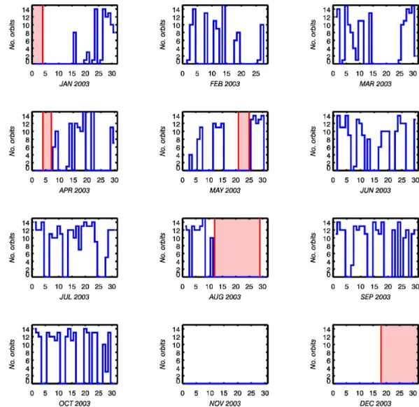
Fig. 1. Number of orbits per day of the year 2003 processed by WFM-DOAS (blue lines). The maximum number of orbits per day is about
14 (∼100%). The red shaded areas indicate the decontamination phases performed to get rid of the ice layer that grows on the near-infrared detectors of channels 7 and 8. Data gaps are due to decontamination but also due to other (mostly ground processing related) reasons.
Atmos. Chem. Phys., 0000, 0001–21, 2005 www.atmos-chem-phys.org/acp/0000/0001/
Fig. 1. Number of orbits per day of the year 2003 processed by WFM-DOAS (blue lines). The maximum number of orbits per day is about
14 (∼100%). The red shaded areas indicate the decontamination phases performed to get rid of the ice layer that grows on the near-infrared detectors of channels 7 and 8. Data gaps are due to decontamination but also due to other (mostly ground processing related) reasons.
elsewhere (Buchwitz et al., 2000a, 2004, 2005). In short, WFM-DOAS is an unconstrained linear-least squares method based on scaling pre-selected trace gas vertical pro-files. The fit parameters are the desired vertical columns. The logarithm of a linearized radiative transfer model plus a low-order polynomial is fitted to the logarithm of the ratio of the measured nadir radiance and solar irradiance spectrum, i.e., observed sun-normalized radiance. The WFM-DOAS refer-ence spectra are the logarithm of the sun-normalized radi-ance and its derivatives. They are computed with a radiative transfer model taking into account line-absorption and mul-tiple scattering (Buchwitz et al., 2000b). A fast look-up table scheme has been developed in order to avoid time consuming on-line radiative transfer simulations. A detailed description of the look-up table is given in Buchwitz and Burrows (2004) (please note that the current version of the look-up table is
based on HITRAN2000/2003 line parameters) (Rothmann et al., 2003). A short description is also provided in Buchwitz et al. (2005).
In order to identify cloud-contaminated ground pixels we use a simple threshold algorithm based on sub-pixel infor-mation as provided by the SCIAMACHY Polarization Mea-surement Devices (PMDs) (details are given in Buchwitz et al., 2004, 2005). We use PMD1 which corresponds to the spectral region 320–380 nm located in the UV part of the spectrum. Strictly speaking, the algorithm detects enhanced backscatter in the UV. Enhanced UV backscatter mainly re-sults from clouds but might also be due to high aerosol load-ing or high surface UV spectral reflectance. As a result, ice or snow covered surfaces may be wrongly classified as cloud contaminated. This needs to be improved in future versions of our retrieval method.
The quality of the WFM-DOAS fits in the near-infrared is poor (i.e., the fit residuals are large) when applying WFM-DOAS to the operational Level 1 data products. In order to improve the quality of the fits and thereby the quality of our data products we pre-process the operational Level 1 data products mainly with respect to a better dark signal calibra-tion (see Buchwitz et al., 2004, 2005). In addicalibra-tion, there are indications that the in-orbit slit function of SCIAMACHY is different from the one measured on-ground (Gloudemans et al., 2005) due to the ice layer (see Sect. 2). We use a slit function that has been determined by applying WFM-DOAS to the in-orbit nadir measurements. We selected the one that resulted in best fits, i.e., smallest fit residuum (see Buchwitz et al., 2004, 2005).
4 WFM-DOAS data products: Time coverage
The WFM-DOAS trace gas column data products have been derived by processing all consolidated SCIAMACHY Level 1 operational product files (i.e., the calibrated and geolocated spectra) of the year 2003 that have been made available by ESA/DLR (up to mid-2004). Figure 1 gives an overview about the number of orbits per day that have been processed. The maximum number of orbits per day is about fourteen. As can been seen (blue lines), all 14 orbits were available for only a small number of days. For many days no data were available. Many of the large data gaps are due to decontami-nation phases (see Sect. 2) which are indicated by red shaded areas. For November and December 2003 no consolidated (i.e., full product) orbit files have been made available (for ground processing related reasons).
5 Carbon monoxide (CO)
CO columns have been retrieved from a small spectral fitting window (2359–2370 nm) located in SCIAMACHY channel 8. The fitting window covers four CO absorption lines. The retrieval is complicated by strong overlapping absorp-tion features of methane and water vapor. The first CO re-sults from SCIAMACHY have been presented in Buchwitz et al. (2004) focusing on a detailed analysis of three days of data of the year 2003. For details concerning pre-processing of the spectra (for improving the calibration), WFM-DOAS v0.4 retrieval, vertical column averaging kernels, quality of the spectral fits, and a quantitative comparison with MO-PITT Version 3 CO columns (Deeter et al., 2003; Emmons et al., 2004) we refer to Buchwitz et al. (2004). An initial error analysis using simulated measurements can be found in Buchwitz et al. (2004) and Buchwitz and Burrows (2004) where it is shown that the retrieval errors are expected to be less than about 20%. In Buchwitz et al. (2004) it has been shown that plumes of elevated CO can be detected with single overpass data in good qualitative agreement with
MOPITT. Globally, for measurements over land, the stan-dard deviation of the difference with respect to MOPITT was shown to be in the range 0.4–0.6×10¹⁸molecules/cm2 and the linear correlation coefficient between 0.4 and 0.7. The differences of the CO from the two sensors depend on time and location but are typically within 30% for most lat-itudes. Perfect agreement with MOPITT is, however, not to be expected for a number of reasons (differences in overpass time, spatial resolution, etc.). In this context it is important to point out that the sensitivity of SCIAMACHY measure-ments is nearly independent of altitude whereas the sensitiv-ity of MOPITT to boundary layer CO is low. On the other hand, retrieval of CO from SCIAMACHY is not unproblem-atic. For example, the WFM-DOAS v0.4 CO columns are scaled with a constant factor of 0.5 to compensate for an ob-vious overestimation (see Buchwitz et al., 2004, for details). This overestimation is most probably closely related to the difficulty of accurately fitting the weak CO lines in the se-lected fitting window (note that the CO columns of our new version 0.5 data product, which is retrieved from a different fitting window, are not scaled any more; see Sect. 9 for de-tails). The fit residuals, which are on the order of the CO lines, are not signal-to-noise limited but dominated by (not yet understood) rather stable spectral artifacts.
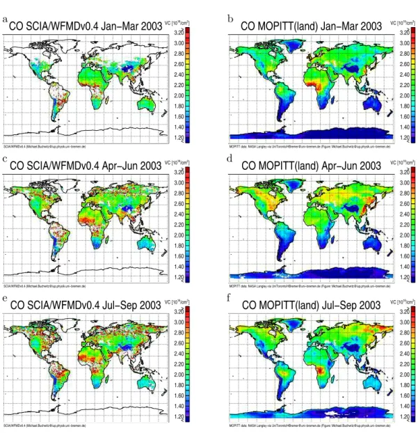
Figure 2 shows a comparison of tri-monthly averaged WFM-DOAS version 0.4 CO columns with CO from MO-PITT (version 3). Because of the low surface reflectivity of water in the NIR (outside sun-glint conditions) the nadir measurements are noisy over the ocean. Therefore, we focus on SCIAMACHY measurements over land. Only these mea-surements are shown in Fig. 2. The same land mask as used for SCIAMACHY has also been used for MOPITT to ease the comparison. SCIAMACHY data have only been included in Fig. 2 if the CO fit error was less than 60% and when the pixels were cloud free. As can be seen from Fig. 1, there are large SCIAMACHY data gaps. Therefore, the SCIA-MACHY data shown in Fig. 2 are not tri-monthly averages obtained from a bias free sampling. For example, the July-September average is strongly weighted towards July and September due to a long decontamination period with no data in August. There are also gaps in the tropical region due to persistent cloud cover. Furthermore, there are no data over Greenland and Antarctica, and over large parts of the North-ern Hemisphere in the period January to March. This is par-tially also due to clouds but mainly due to ice/snow covered surfaces because of the limitations of the cloud detection al-gorithm.
When comparing the January–March data from SCIA-MACHY and MOPITT one can see that there are similari-ties but also differences. For example, the inter-hemispheric difference is clearly visible for MOPITT but barely visible for SCIAMACHY. Both sensors see low columns over re-gions of elevated surface topography (Himalaya, Andes and Rocky Mountains) and high columns over the western part of central Africa (where significant biomass burning is going
M. Buchwitz et al.: CO, CH4, and CO2columns from SCIAMACHY 3317
M. Buchwitz et al.: CO, CH4, and CO2columns from SCIAMACHY 13
a b
CO SCIA/WFMDv0.4 Jan−Mar 2003
< 1.20 1.40 1.60 1.80 2.00 2.20 2.40 2.60 2.80 3.00 3.20 > < 1.20 1.40 1.60 1.80 2.00 2.20 2.40 2.60 2.80 3.00 3.20 > VC [1018/cm2] SCIA/WFMDv0.4 ([email protected]−bremen.de)CO MOPITT(land) Jan−Mar 2003
< 1.20 1.40 1.60 1.80 2.00 2.20 2.40 2.60 2.80 3.00 3.20 > < 1.20 1.40 1.60 1.80 2.00 2.20 2.40 2.60 2.80 3.00 3.20 > VC [1018/cm2]MOPITT data: NASA Langley via UniToronto/HBremer@uni−bremen.de (Figure: [email protected]−bremen.de)
c d
CO SCIA/WFMDv0.4 Apr−Jun 2003
< 1.20 1.40 1.60 1.80 2.00 2.20 2.40 2.60 2.80 3.00 3.20 > < 1.20 1.40 1.60 1.80 2.00 2.20 2.40 2.60 2.80 3.00 3.20 > VC [1018/cm2] SCIA/WFMDv0.4 ([email protected]−bremen.de)CO MOPITT(land) Apr−Jun 2003
< 1.20 1.40 1.60 1.80 2.00 2.20 2.40 2.60 2.80 3.00 3.20 > < 1.20 1.40 1.60 1.80 2.00 2.20 2.40 2.60 2.80 3.00 3.20 > VC [1018/cm2]MOPITT data: NASA Langley via UniToronto/HBremer@uni−bremen.de (Figure: [email protected]−bremen.de)
e f
CO SCIA/WFMDv0.4 Jul−Sep 2003
< 1.20 1.40 1.60 1.80 2.00 2.20 2.40 2.60 2.80 3.00 3.20 > < 1.20 1.40 1.60 1.80 2.00 2.20 2.40 2.60 2.80 3.00 3.20 > VC [1018/cm2] SCIA/WFMDv0.4 ([email protected]−bremen.de)CO MOPITT(land) Jul−Sep 2003
< 1.20 1.40 1.60 1.80 2.00 2.20 2.40 2.60 2.80 3.00 3.20 > < 1.20 1.40 1.60 1.80 2.00 2.20 2.40 2.60 2.80 3.00 3.20 > VC [1018/cm2]MOPITT data: NASA Langley via UniToronto/HBremer@uni−bremen.de (Figure: [email protected]−bremen.de)
Fig. 2. Tri-monthly averaged CO columns over land from SCIAMACHY/ENVISAT (left) and MOPITT/EOS-Terra (right). Only the columns
over land are shown because the quality of the SCIAMACHY CO columns over water is low due to the low reflectivity of water in the near-infrared. For SCIAMACHY only data have been averaged where the CO fit error is less than 60% and where the PMD1 cloud identification algorithm indicates a cloud free pixel. For MOPITT cloudy pixels are also not included.
www.atmos-chem-phys.org/acp/0000/0001/ Atmos. Chem. Phys., 0000, 0001–21, 2005
Fig. 2. Tri-monthly averaged CO columns over land from SCIAMACHY/ENVISAT (left) and MOPITT/EOS-Terra (right). Only the columns
over land are shown because the quality of the SCIAMACHY CO columns over water is low due to the low reflectivity of water in the near-infrared. For SCIAMACHY only data have been averaged where the CO fit error is less than 60% and where the PMD1 cloud identification algorithm indicates a cloud free pixel. For MOPITT cloudy pixels are also not included.
on during the dry season), south-east Asia, parts of Europe, and the south-eastern part of the United States of Amer-ica. Over South America and the northern part of Australia SCIAMACHY sees elevated CO not observed by MOPITT.
During April to June both sensors see elevated CO over large parts of the Northern Hemisphere (eastern part of the US, Canada, western Europe and large parts of Russia (the observed pattern are, however, not exactly identical), south-east Asia and parts of China. Over India and parts of south-east Asia SCIAMACHY sees elevated CO not seen by MOPITT. The largest difference over the Northern Hemi-sphere occurs over the western part of central Africa where the CO retrieved from SCIAMACHY is significantly higher than the CO from MOPITT. The reason for the elevated
SCIAMACHY CO columns over the Sahel region is not yet exactly understood but it is very likely that this is an over-estimation due to systematic artifacts (caused by, for exam-ple, aerosol). This is supported by the fact that our new ver-sion 0.5 CO WFM-DOAS data product, which is shortly de-scribed in Sect. 9, shows significantly lower values over this region compared to v0.4. The version 0.5 CO columns are less sensitive to errors related to average light path (or ob-served airmass) uncertainty resulting from the unknown dis-tribution of scattering material (aerosols, clouds) in the atmo-sphere and/or surface reflectivity variability. The reason for this is that the CO v0.5 column is normalized by the methane column obtained from the same spectral fitting window re-sulting in (at least partial) canceling of errors. Also over large
3318 M. Buchwitz et al.: CO, CH4, and CO2columns from SCIAMACHY
Fig. 3. The black diamonds show XCH4(v0.4) as measured by SCIAMACHY over the Sahara normalized by a constant reference value of 1750 ppbv as a function of day of the year 2003 (”methane bias curve”). The red diamonds (”Transmission (orig.)”) show independent measurements, namely the SCIAMACHY channel 8 transmission which changes due to the varying ice layer on the detector. This curve has been determined by averaging the signal of the solar measurements and normalizing it. The magenta (m) ”Transmission (transformed)” curve has been obtained by a linear transformation of the red (r) curve, i.e., by computing m = A + B r. Applying the same coefficients A and B as used for the data before day 230 also to the data after day 230 results in the yellow curve which still shows an offset with respect to the black methane bias curve. To get a better match, two sets of coefficients have been used, one for the data before day 230 and another set for the data after day 230. The reason why different coefficients are needed is most probably because the spatial distribution of the ice layer on the detector changes with time.
Atmos. Chem. Phys., 0000, 0001–21, 2005 www.atmos-chem-phys.org/acp/0000/0001/
Fig. 3. The black diamonds show XCH4(v0.4) as measured by
SCIAMACHY over the Sahara normalized by a constant reference value of 1750 ppbv as a function of day of the year 2003 (“methane bias curve”). The red diamonds (“Transmission (orig.)”) show inde-pendent measurements, namely the SCIAMACHY channel 8 trans-mission which changes due to the varying ice layer on the detector. This curve has been determined by averaging the signal of the solar measurements and normalizing it. The magenta (m) “Transmission (transformed)” curve has been obtained by a linear transformation of the red (r) curve, i.e., by computing m=A+B r. Applying the same coefficients A and B as used for the data before day 230 also to the data after day 230 results in the yellow curve which still shows an offset with respect to the black methane bias curve. To get a bet-ter match, two sets of coefficients have been used, one for the data before day 230 and another set for the data after day 230. The rea-son why different coefficients are needed is most probably because the spatial distribution of the ice layer on the detector changes with time.
parts of South America the SCIAMACHY measurements are significantly higher than MOPITT (WFM-DOAS version 0.5 also shows higher values than MOPITT confirming the v0.4 results). For the time period July to September the pattern of elevated CO as observed by SCIAMACHY is similar to the SCIAMACHY observations during April to June. The main differences are: (i) higher values over Southern Amer-ica (in quantitative agreement with MOPITT; note that this is the time where most of the biomass burning takes place in this area) and (ii) higher values over the eastern part of northern Russia (also observed by MOPITT). There are also significant differences when comparing the SCIAMACHY data with MOPITT especially over the northern part of cen-tral Africa, the eastern US, south-east Asia and over most of the mid to high latitude parts of the Northern Hemisphere.
In summary, the agreement with MOPITT is reasonable but there are large differences at certain locations during cer-tain times of the year. More investigations are needed to ex-plain the observed differences taking into account the differ-ent altitude sensitivities of both sensors.
6 Methane (CH4)
The methane columns have been retrieved from a small spectral fitting window (2265–2280 nm) located in SCIAMACHY channel 8 which covers several absorption lines of CH4and several (much weaker) absorption lines of
nitrous oxide (N2O) and water vapor (H2O). The main
sci-entific application of the methane measurements of SCIA-MACHY is to obtain information on the surface sources of methane. The modulation of methane columns due to methane sources is only on the order of a few percent. This is much weaker than the variation of the methane column due to changes of surface pressure / surface elevation (be-cause methane is well-mixed the methane column is highly correlated with the total air mass over a given location and, therefore, with surface pressure). To filter out these much larger disturbing modulations, the methane columns need to be normalized by the observed airmass to obtain a so called dry air column averaged mixing ratio of methane (denoted XCH4). To accomplish this, oxygen (O2) columns have been
retrieved in addition to the methane columns. From the oxy-gen columns the airmass can be calculated using its constant mixing ratio of 0.2095. The O2columns used to compute the
WFM-DOAS v0.4 XCH4 data product have been retrieved
from the SCIAMACHY measurements in the O2 A band
spectral region (around 760 nm; channel 4).
First CH4results from SCIAMACHY have been presented
in Buchwitz et al. (2005) focusing on a detailed analysis of four days of data of the year 2003. For details concerning pre-processing of the spectra (to improve the calibration), WFM-DOAS (v0.4) processing, averaging kernels, quality of the spectral fits, an initial error analysis (see also Buch-witz and Burrows, 2004), and a quantitative comparison with global models we refer to that study. According to the er-ror analysis erer-rors of a few percent due to undetected cirrus clouds, aerosols, surface reflectivity, temperature and pres-sure profiles, etc., are to be expected. It has been shown in Buchwitz et al. (2005) that the WFM-DOAS Version 0.4 methane columns have a time dependent (nearly globally uniform) bias of up to –15% (low bias of SCIAMACHY) for one of the four days that have been analyzed. The bias is correlated with the time after the last decontamination per-formed to get rid of the ice layers on the detector. There-fore, Buchwitz et al. (2005) concluded that the bias might be due to the “ice-issue” (see Sect. 2). This is consistent with the finding of Gloudemans et al. (2005) that the ice build-up on the detectors results in a broadening of the instrument slit function (the wider the slit function compared to the assumed
M. Buchwitz et al.: CO, CH4, and CO2columns from SCIAMACHY 3319
M. Buchwitz et al.: CO, CH4, and CO2columns from SCIAMACHY 15
a
b
c
d
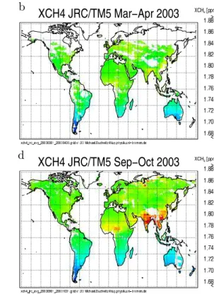
Fig. 4. Column averaged mixing ratios of methane (XCH4) as measured by SCIAMACHY over land using WFM-DOAS v0.41 (left) compared to TM5 model data (right). For SCIAMACHY only the measurements from cloud free pixels have been averaged where the methane error is less than 10%. The model data have been averaged taking into account the daily sampling of the SCIAMACHY data. The model data have been scaled by a constant factor of 1.03 to compensate for the bias between the two data sets (see Fig. 5).
www.atmos-chem-phys.org/acp/0000/0001/ Atmos. Chem. Phys., 0000, 0001–21, 2005
Fig. 4. Column averaged mixing ratios of methane (XCH4) as measured by SCIAMACHY over land using WFM-DOAS v0.41 (left)
compared to TM5 model data (right). For SCIAMACHY only the measurements from cloud free pixels have been averaged where the methane error is less than 10%. The model data have been averaged taking into account the daily sampling of the SCIAMACHY data. The model data have been scaled by a constant factor of 1.03 to compensate for the bias between the two data sets (see Fig. 5).
slit function, the larger the underestimation of the retrieved methane column).
Typically, the weak methane source signal is difficult to be clearly detected with single overpass or single day SCIA-MACHY data. For accurate detection of methane sources averages have to be computed. Because of the time depen-dent bias of the WFM-DOAS v0.4 methane columns this is, however, not directly possible.
In the following we describe how we have processed the SCIAMACHY data to get an improved version of our methane data product (Version 0.41) by applying a bias cor-rection to the v0.4 methane columns. We assume that the data can be sufficiently corrected by dividing the columns by a globally constant scaling factor which only depends on time (on the day of the measurement). The correction fac-tor has been determined as follows: For each day all cloud free v0.4 XCH4 measurements over the Sahara have been
averaged. The ratio of these daily average mixing ratios to a constant reference value (chosen to be 1750 ppbv) is approx-imately the methane bias (because methane is not constant this is not exactly the methane bias and a certain systematic error is introduced by this assumption). This time depen-dent methane bias is shown in Fig. 3 (black diamonds). This bias shows a similar time dependence as the independently
measured channel 8 transmission loss also shown in Fig. 3 (red diamonds). The transmission has been determined by averaging the signal of the channel 8 solar measurements normalized to a reference measurement at the beginning of the mission. The varying transmission is a consequence of the varying ice layer on the detectors. Figure 3 shows a third curve, the (daily) correction factor (magenta diamonds). The correction factor curve has been obtained by linearly trans-forming the transmission curve. The coefficients of the lin-ear transformation have been selected such that a good match is obtained with the methane bias curve. In order to correct the WFM-DOAS v0.4 methane columns for the systematic errors introduced by the ice layer the correction factors are applied as follows: All v0.4 methane columns of a given day have been divided by the correction factor for this day. The corrected WFM-DOAS v0.4 methane columns are the new WFM-DOAS v0.41 (absolute) methane columns.
In order to generate the new WFM-DOAS v0.41 XCH4
product a second modification has been applied: Instead of normalizing the methane columns by the oxygen column re-trieved from the 760 nm O2A band (as done for v0.4 XCH4),
they have been normalized by the CO2 columns retrieved
from the 1580 nm region (for details on CO2 retrieval see
methane columns has been first proposed by Frankenberg et al. (2005c) (the approach has been presented earlier, namely at the ENVISAT Symposium, Salzburg, Austria, September 2004).
The reason why normalizing methane by CO2rather than
O2 is expected to give better results for XCH4 is that the
CO2band is located spectrally much closer to the CH4band
than the O2A band. Retrieval errors due to aerosols, residual
cloud contamination, surface reflectivity uncertainties, etc., are expected to be the more similar, the more similar the ra-diative transfer is (including all parameters that influence the radiative transfer such as surface albedo). In general, this requires that the two spectral intervals from which the two columns are retrieved are spectrally located as close as pos-sible next to each other (there are exceptions, of course, for example in case of spectral absorption features). As the CO2
fitting window (at 1580 nm), is much closer to the CH4fitting
window (2270 nm) than the O2window (760 nm) canceling
of errors will be better using CO2. In addition, when the
column retrieval from the two spectral regions suffers from similar instrumental/calibration errors, also these errors can-cel to a certain extent (note that in Sect. 9 we shortly describe our latest XCH4data product (v0.5) derived using methane
columns retrieved from channel 6, i.e., located close to the CO2 fitting window (also channel 6) to improve the
can-celling of errors Frankenberg et al., 2005c).
The drawback of this approach is that CO2is not as
con-stant as O2mainly because of the surface sources and sinks
of CO2. This approach requires that the variability of the
col-umn averaged mixing ratio of CO2is small (ideally
negligi-ble) compared to the variability of the column averaged mix-ing ratio of CH4. According to global model simulation this
is a reasonable assumption. The model simulations shown in Buchwitz et al. (2005) indicate that the variability of the methane column is about 6% (±100 ppbv) and the variability of the CO2column is about 1.5% (±5 ppmv), i.e., a factor of
four smaller than for methane. This means that the error in-troduced by essentially assuming that CO2is constant is less
than about 1.5%. This is comparable to the estimated error on the WFM-DOAS v0.4 CO2columns as reported in
Buch-witz et al. (2005). It has to be pointed out, however, that this aspects needs more study as, for example, the XCO2results
from SCIAMACHY presented in Sect. 7 show a significantly higher XCO2variability compared to model simulations.
Figure 4 shows a comparison of WFM-DOAS v0.41 XCH4 with TM5 model simulations. The TM5 model is a
two-way nested atmospheric zoom model (Krol et al., 2005). It allows to define zoom regions (e.g. over Europe) which are run at higher spatial resolution (1×1 deg), embedded into the global domain, run at a resolution of 6×4 deg. We employ the tropospheric standard version of TM5 with 25 vertical layers. TM5 is an off-line model and uses analyzed meteo-rological fields from the ECMWF weather forecast model to describe advection and vertical mixing by cumulus convec-tion and turbulent diffusion. CH4(a priori) emissions are as
described by Bergamaschi et al. (2005). Chemical destruc-tion of CH4by OH radicals is simulated using pre-calculated
OH fields based on CBM-4 chemistry and optimized with methyl chloroform. For the stratosphere also the reaction of CH4with Cl and O(1D) radicals are considered. The
compar-ison is limited to observations over land as the SCIAMACHY observations over ocean are less precise because of the low ocean reflectivity in the near-infrared. For SCIAMACHY all measurements from cloud free pixels have been averaged where the CH4 column fit error is less than 10%. The
bi-monthly averages have been computed from daily gridded data. For the model simulations only those grid boxes where measurements were available have been used to compute the averages.
The comparison with the model simulations shows simi-larities but also differences. Very interestingly and in qual-itative agreement with the model simulations, the measure-ments show high CH4mixing ratios in the September to
Oc-tober 2003 average over India, southeast Asia, and over the western part of central Africa, which are absent or signifi-cantly lower in the March to April average. In the model the high columns over these regions are a result of methane emissions mainly from rice fields, wetlands, ruminants, and waste handling. The good agreement with the model simula-tions indicates that SCIAMACHY can detect these emission signals. Similar findings have been reported in Frankenberg et al. (2005c). However, there are also differences compared to the model simulations. For example, in the March–April average the SCIAMACHY data are a few percent higher over large parts of northern South America. Over large parts of the Northern Hemisphere the SCIAMACHY data are a few percent lower.
We have also compared monthly averaged v0.41 XCH4
with (the throughput-based) bias corrected v0.4 XCH4to
as-sess the impact of normalizing by CO2(as done for v0.41)
compared to normalizing by O2(as done for v0.4). For
ex-ample for October 2003 this comparison showed significant differences. The extended plumes of high v0.41 XCH4over
India, China, and central Africa (similar as those shown in Fig. 4) do not show up so clearly in the v0.4 XCH4. In
ad-dition, there are also large differences at other places with the v0.4 XCH4being more “noisy” (more inhomogeneous)
than V0.41 XCH4. This confirms that cancellation of errors
is better for v0.41 XCH4 (normalization by CO2) than for
v0.4 XCH4(normalization by O2). The impact of using the
O2measurements to obtain column averaged mixing ratios is
further discussed in Sect. 7 where it has been used to obtain XCO2.
Figure 5 shows a quantitative comparison of the global daily data with the TM5 model, the correlation coefficient and the bias for the two versions of SCIAMACHY XCH4
data products, namely v0.4 and v0.41. As can be seen, the bias is significantly smaller for the v0.41 data, although not zero. There still appears to be a systematic bias due to the ice issue indicating that the bias correction applied to generate
M. Buchwitz et al.: CO, CH4, and CO2columns from SCIAMACHY 3321
16 M. Buchwitz et al.: CO, CH4, and CO2columns from SCIAMACHY
Fig. 5. Comparison of daily SCIAMACHY XCH4measurements (versions 0.4 (blue triangles) and 0.41 (black diamonds)) with TM5 model
simulations. The top panel shows the bias (SCIAMACHY-model), the middle panel the standard deviation of the difference, and the bottom panel Pearson’s linear correlation coefficient r.
Atmos. Chem. Phys., 0000, 0001–21, 2005 www.atmos-chem-phys.org/acp/0000/0001/
Fig. 5. Comparison of daily SCIAMACHY XCH4measurements (versions 0.4 (blue triangles) and 0.41 (black diamonds)) with TM5 model
simulations. The top panel shows the bias (SCIAMACHY-model), the middle panel the standard deviation of the difference, and the bottom panel Pearson’s linear correlation coefficient r.
the v0.41 data is not perfect. Also the correlation with the model results is typically significantly better for the version 0.41 data.
7 Carbon dioxide (CO2)
The CO2columns have been retrieved using a small spectral
fitting window (1558–1594 nm) located in SCIAMACHY channel 6 (which is not affected by an ice layer). This spec-tral region covers one absorption band of CO2and weak
ab-sorption features of water vapor. As for methane v0.4 (air or)
O2-normalized CO2columns have been derived, the dry air
column averaged mixing ratios XCO2. First results of CO2
from SCIAMACHY have been presented in Buchwitz et al. (2005). For details concerning pre-processing of the spectra (for improving the calibration), WFM-DOAS (v0.4) process-ing, vertical column averaging kernels, quality of the spectral fits, and a quantitative comparison with global model simu-lations we refer to Buchwitz et al. (2005). An initial error analysis using simulated measurements is given in Buchwitz et al. (2005) and Buchwitz and Burrows (2004). According to this analysis, errors of a few percent due to undetected
cirrus clouds, aerosols, surface reflectivity, temperature and pressure profiles, etc., are to be expected. To compensate for a not yet understood systematic underestimation of the initially retrieved CO2columns the WFM-DOAS v0.4 CO2
columns have been scaled with a constant factor of 1.27 (see Buchwitz et al., 2005, for details). The factor has been cho-sen to make sure that the CO2 column is near its expected
value of about 8×10²¹molecules/cm2for a cloud free scene with a surface elevation close to sea level and moderate sur-face albedo. In Buchwitz et al. (2005) it has been shown that the WFM-DOAS v0.4 CO2(scaled) columns agree with
model columns within a few percent (range –3.7% to +2.0%). Because of the scaling factor a meaningful comparison with reference data should focus on variability in time and space and not on the absolute level. Also the v0.4 O2 columns,
used to compute XCO2, are scaled (by 0.85). The reason
for the about 15% overestimation of the originally retrieved O2columns is currently unclear. The factor has been chosen
to make sure that the O2 column is near its expected value
of about 4.5×1024molecules/cm2for a cloud free scene with a surface elevation close to sea level and moderate surface albedo. In a recent paper of van Diedenhofen et al. (2005) an overestimation of 2–5% over scenes with moderate to high surface albedo is found when comparing their SCIAMACHY O2columns with actual meteorological data. They found that
2% can be explained by an offset on the measured reflectance and argue that the remaining overestimation is likely due to aerosols. Taking this into account our retrievals are still over-estimated by 10%. At present we cannot offer an explana-tions for this discrepancy. The investigation of this will be a focus of our future work. For now we have to state that the v0.4 CO2and O2columns are scaled resulting in a quite
large scaling factor for XCO2of 1.49 (=1.27/0.85). Because
of this we focus on variability rather than on absolute XCO2
levels when comparing our XCO2to reference data.
In Buchwitz et al. (2005) it has been shown that the spa-tial and temporal pattern of the retrieved column averaged mixing ratio is in reasonable agreement with the model data except for the amplitude of the variability. The measured variability is about a factor of four higher than the variabil-ity of the model data (about 6% compared to about 1.5% for the model data). This is also confirmed in this study which provides more details on this finding. In this con-text it is important to note that an overestimation of the re-trieved variability of about a factor 2.2 (at maximum) may be explained as follows: The SCIAMACHY/WFM-DOAS CO2 column averaging kernels (shown in Buchwitz et al.,
2005) peak in the lower troposphere and have a maximum value of about 1.5. This means that the retrieved variabil-ity is overestimated by 50% (e.g., 3 ppmv instead of 2 ppmv) if this column variability is entirely due to variability in the lower troposphere (note that the averaging kernels typically decrease with altitude and reach 1.0 (i.e., no over- or under-estimation) around 400 hPa (∼7 km); above 400 hPa they are less than 1.0). The scaling factor of 1.49 which is currently
applied to the retrieved XCO2may also contribute to an
en-hancement of the retrieved variability. This however requires that the initially retrieved columns are off by a constant off-set rather than a constant scaling factor (this aspect needs further investigation). The averaging kernels in combination with the scaling factor might explain at maximum a factor of 2.2 (=1.5×1.49) overestimated variability. The different resolution of the SCIAMACHY measurements (60×30 km2) and the model simulations (1.8×1.8 deg) also contribute to a difference in the observed and the modeled variability. Fur-ther study is needed to identify the origin of the scaling fac-tors for CO2and O2. Also the averaging kernels need to be
taken into account when comparing with reference data. The factor of 2.2 however can only partially explain the observed variability. At least a factor of 2 higher observed variability still needs to be explained.
In the following we present a detailed comparison of the retrieved XCO2 with TM3 model simulations. TM3 3.8
(Heimann and K¨orner, 2003) is a three-dimensional global atmospheric transport model for an arbitrary number of ac-tive or passive tracers. It uses re-analyzed meteorological fields from the National Center for Environmental Predic-tion (NCEP) or from the ECMWF re-analysis. The modeled processes comprise tracer advection, vertical transport due to convective clouds and turbulent vertical transport by diffu-sion. Available horizontal resolutions range from 8×10 deg to 1.1×1.1 deg. In this case, TM3 was run with a resolu-tion of 1.8×1.8 deg and 28 layers, and the meteorology fields were derived from the NCEP/DOE AMIP-II reanalysis. CO2
source/sink fields for the ocean originate from Takahaschi et al. (2002), for anthropogenic sources from the EDGAR 3.2 database and for the biosphere from the BIOME-BGC model (Thornton et al., 2002) with inclusion of a simple parameter-ization of the diurnal cycle in photosynthesis and respiration. For SCIAMACHY the averages have been computed using only the cloud free pixels with a XCO2 error of less than
10%. Shown in Fig. 6 are only the data over land because of the problems with measuring over the ocean in the near-infrared (see Sect. 5).
For SCIAMACHY Fig. 6 shows absolute column aver-aged mixing ratios of CO2in the range 335–385 ppmv. For
TM3 “uncalibrated” XCO2-offsets are shown which are in
the range 0–13.7 ppmv. These offsets do not include the (current) background concentration of CO2. Therefore, not
the absolute values but only the variability in space and time should be compared. The model simulations show low CO2
columns (compared to the mean column) over the Northern Hemisphere in July 2003 compared to higher values in May and September. This is mainly due to uptake of CO2by the
biosphere which results in minimum columns around July. Qualitatively the SCIAMACHY data show a similar time de-pendence with also lower columns in July compared to May and September. Thus the general time dependence of the SCIAMACHY retrievals is consistent with the model simu-lations.
M. Buchwitz et al.: CO, CHM. Buchwitz et al.: CO, CH4, and CO4, and CO2columns from SCIAMACHY2columns from SCIAMACHY 17 3323
Fig. 6. Comparison of SCIAMACHY XCO2(left) with TM3 model simulations (right). For SCIAMACHY all cloud free measurements over land have been averaged where the CO2column fit error is less than 10%. For TM3 monthly averaged XCO2-offsets are shown. These offsets do not include the background concentration of CO2. Therefore, only the spatial and temporal variability should be compared. Two different scales have been used, one for SCIAMACHY (±25 ppmv) and one for the model simulations (±6.85 ppmv), to consider the 3-4 times higher variability of the SCIAMACHY data compared to the model data.
www.atmos-chem-phys.org/acp/0000/0001/ Atmos. Chem. Phys., 0000, 0001–21, 2005
Fig. 6. Comparison of SCIAMACHY XCO2(left) with TM3 model simulations (right). For SCIAMACHY all cloud free measurements
over land have been averaged where the CO2column fit error is less than 10%. For TM3 monthly averaged XCO2-offsets are shown. These
offsets do not include the background concentration of CO2. Therefore, only the spatial and temporal variability should be compared. Two
different scales have been used, one for SCIAMACHY (±25 ppmv) and one for the model simulations (±6.85 ppmv), to consider the 3–4 times higher variability of the SCIAMACHY data compared to the model data.
Figure 6 shows that over large parts of the (mostly west-ern) Sahara SCIAMACHY sees “plumes” of relatively high CO2(red colored areas) not present in the model simulations.
These few percent too high CO2 mixing ratios may result
from the high surface reflectivity over the Sahara in combina-tion with aerosol variability. This is qualitatively consistent with the analysis of Houweling et al. (2005) who performed a detailed study on the impact of aerosols and albedo on SCIA-MACHY CO2column retrievals. We are optimistic that this
problem can be substantially reduced in future versions of
our retrieval algorithm which currently only considers first order effects of albedo and aerosol variability (mainly by in-cluding a polynomial in our WFM-DOAS fit). Currently, for the radiative transfer simulations, a constant surface albedo of 0.1 is assumed and only one aerosol scenario. Accord-ing to the error analysis presented in Buchwitz et al. (2005) the XCO2 error is estimated to be +4.5% (16 ppmv
over-estimation) if the albedo is 0.3 instead of 0.1 (for a solar zenith angle of 50◦). Depending on the aerosol scenario and on a number of other parameters the actual error might be
3324 M. Buchwitz et al.: CO, CH4, and CO2columns from SCIAMACHY
Fig. 7. Comparison of daily gridded XCO2from SCIAMACHY (considering only cloud free pixels over land) with TM3 model simulations (considering only those gridboxes for a given day where also observations have been made). First three panels: Black diamonds: SCIA-MACHY daily average. Blue triangles: as black diamonds but for TM3. Solid lines: 31 days running means of the daily data. Red lines: as black lines but using the TM3 surface pressure (instead of the retrieved O2column) to convert the retrieved CO2column to XCO2. The top panel shows a comparison of northern hemispheric averages, the middle panel a comparison of southern hemispheric averages, and the bottom panel a comparison of the inter-hemispheric differences (northern hemispheric mean minus southern hemispheric mean). Last three panels: The top panel shows the mean difference (SCIA-TM3) for the global data, the middle panel the standard deviation of this difference, and the bottom panel Pearson’s linear correlation coefficient for the two data sets.
Atmos. Chem. Phys., 0000, 0001–21, 2005 www.atmos-chem-phys.org/acp/0000/0001/
Fig. 7. Comparison of daily gridded XCO2from SCIAMACHY (considering only cloud free pixels over land) with TM3 model simulations (considering only those gridboxes for a given day where also observations have been made). First three panels: Black diamonds: SCIA-MACHY daily average. Blue triangles: as black diamonds but for TM3. Solid lines: 31 days running means of the daily data. Red lines: as black lines but using the TM3 surface pressure (instead of the retrieved O2column) to convert the retrieved CO2column to XCO2. The
top panel shows a comparison of northern hemispheric averages, the middle panel a comparison of southern hemispheric averages, and the bottom panel a comparison of the inter-hemispheric differences (northern hemispheric mean minus southern hemispheric mean). Last three panels: The top panel shows the mean difference (SCIA-TM3) for the global data, the middle panel the standard deviation of this difference, and the bottom panel Pearson’s linear correlation coefficient for the two data sets.
somewhat higher or lower. This indicates that the high val-ues seen by SCIAMACHY over the Sahara may be explained by retrieval algorithm limitations as the current version does not take albedo and aerosol variations fully into account.
To provide more confidence that the uptake (and re-lease) of CO2by the biosphere can be observed with
SCIA-MACHY, the year 2003 XCO2data set has been investigated
in more detail. This is important, because the estimated re-trieval errors are on the same order as the few ppmv XCO2
variations shown by the model. It has to be made sure that the observed XCO2 modulations are not an artifact
result-ing from, e.g., solar zenith angle dependent errors. Figure 7 shows a detailed comparison of the daily data as well as for time averaged data (using a 31 days running mean) for the entire year 2003 data set.
Before we discuss the first three panels we will discuss the bottom part of Fig. 7. The last three panels show the mean difference between SCIAMACHY (black) and TM3 (blue),
M. Buchwitz et al.: CO, CH4, and CO2columns from SCIAMACHY 3325
the standard deviation of the difference, and the correlation coefficient. The mean difference is in the range -5 ppmv to –20 ppmv (–1.5% to –5.5%; low bias of SCIAMACHY), the standard deviation is in the range 15–20 ppmv (∼4–5%), and the correlation coefficient is typically around 0.3. The red lines correspond to the same comparison, except that the CO2
columns have been normalized by the surface pressure of the TM3 model to obtain the observed XCO2. As one can see,
using the models surface pressure instead of the retrieved O2
column leaves the results either nearly unchanged (correla-tion coefficient) or results in larger differences (larger bias and standard deviation). From this one can conclude that normalizing the CO2by O2gives better results than
normal-ization by model surface pressure although the normalnormal-ization by O2is not unproblematic because the large spectral
differ-ence between the O2 A band (760 nm) and the CO2 band
(1580 nm) does not guarantee perfect cancellation of errors. The first three panels of Fig. 7 show a comparison of hemi-spheric averages of the two data sets. The data are plotted as anomalies, i.e., each data set has a mean value of zero. The SCIAMACHY data are shown in black, the TM3 data in blue. The symbols refer to daily mean values and the lines to time averaged data (31 days running means). The red lines have the same meaning as described in the previous para-graph (XCO2from SCIAMACHY obtained by normalizing
with TM3 surface pressure). The top panel shows a com-parison of northern hemispheric averages, the second panel the comparison for the Southern Hemisphere, and the third panel a comparison of the inter-hemispheric difference (NH-SH). Let us focus on the time averaged data (solid lines). In the top panel the blue lines show the time dependence of the model XCO2. During the first half of the year
(un-til around day 160) the model XCO2 is mostly larger than
the average (which is zero), during the second half of the year the model XCO2is mostly lower than the average. The
minimum occurs end of July / beginning of August, after the peak in the Northern Hemisphere land biosphere uptake. The SCIAMACHY data (black solid line) show a similar time de-pendence (except at the beginning of the year where the ob-served XCO2is rather constant but the model XCO2slightly
increases with time). Both curves cross the zero line at nearly the same day. The main difference is the amplitude of the si-nusoidal time dependence, which is about a factor of four larger for SCIAMACHY (8 ppmv compared to 2–3 ppmv). The second panel shows the same comparison but for the Southern Hemisphere. The main difference with respect to the Northern Hemisphere is the expected six-month shift and the much smaller amplitude of the time dependence of the observed XCO2 (which is also “noisier”, i.e., shows more
deviation from the smooth sinusoidal behavior of the model simulations). This is most probably due to less available data points for the Southern Hemisphere which contains less land surfaces than the Northern Hemisphere (remember that only data over land are compared). Over the Southern Hemi-sphere the amplitude of the observed variability is roughly
M. Buchwitz et al.: CO, CH4, and CO2columns from SCIAMACHY 19
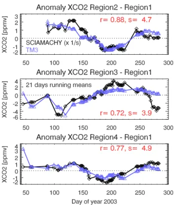
Fig. 8. Comparison of time series of regional XCO2differences (shown as anomalies, i.e., with a mean value of zero). Top panel: The SCIAMACHY data (shown in black) have been obtained as follows: Two regions have been defined (each 20 deg latitude × 20 deg longitude) which are denoted region 1 (the reference region) and region 2 (both regions are shown in Fig.9 where, for example, the reference region is shown as green rectangle). For each region its daily average XCO2has been determined (considering only measurements over land). The daily time series for the reference region has been subtracted from the time series of region 2 (only if data were available for both regions; if not the day was ignored). The time series of the XCO2difference has been smoothed (21 days running mean). Finally, the mean of the time series has been subtracted. The blue curve has been obtained by applying the same procedure to the TM3 model data. Annotation: r denotes Pearson’s linear correlation coefficient and s is a scaling factor obtained from a linear least squares fit of the SCIAMACHY time series to the TM3 time series (s=4.7 means that the SCIAMACHY XCO2anomaly time series has to be divided by 4.7 to match the TM3 time series). The middle and the bottom panels show the corresponding time series for two other regions denoted regions 3 and 4 (shown in Fig. 9).
www.atmos-chem-phys.org/acp/0000/0001/ Atmos. Chem. Phys., 0000, 0001–21, 2005
Fig. 8. Comparison of time series of regional XCO2differences
(shown as anomalies, i.e., with a mean value of zero). Top panel: The SCIAMACHY data (shown in black) have been obtained as follows: Two regions have been defined (each 20-deg latitude × 20-deg longitude) which are denoted region 1 (the reference region) and region 2 (both regions are shown in Fig. 9 where, for example, the reference region is shown as green rectangle). For each region its daily average XCO2has been determined (considering only
mea-surements over land). The daily time series for the reference region has been subtracted from the time series of region 2 (only if data were available for both regions; if not the day was ignored). The time series of the XCO2 difference has been smoothed (21 days running mean). Finally, the mean of the time series has been sub-tracted. The blue curve has been obtained by applying the same procedure to the TM3 model data. Annotation: r denotes Pear-son’s linear correlation coefficient and s is a scaling factor obtained from a linear least squares fit of the SCIAMACHY time series to the TM3 time series (s=4.7 means that the SCIAMACHY XCO2
anomaly time series has to be divided by 4.7 to match the TM3 time series). The middle and the bottom panels show the corresponding time series for two other regions denoted regions 3 and 4 (shown in Fig. 9).
in agreement with the modeled variability. The third panel shows the observed and modeled inter-hemispheric XCO2
difference.
The first three panels of Fig. 7 show that the SCIA-MACHY observations are significantly correlated with the model results. The time dependence of the observed XCO2
cannot be explained by a solar zenith angle dependent er-ror. Over the Northern Hemisphere the minimum solar zenith
3326 M. Buchwitz et al.: CO, CH4, and CO2columns from SCIAMACHY
Fig. 9. Correlation coefficient r (top panel) and scaling factor s (bottom panel) for SCIAMACHY and TM3 time series of regional XCO2
differences (see Fig. 8 for a detailed explanation). The green area indicates the reference region (region 1). Details for regions 2-4 are shown in Fig. 8. The correlation coefficient is only shown for those regions where the final time series comprises at least 70 days. The scaling factor (bottom panel) is only shown for a subset of the regions shown in the top panel, namely only for regions where the correlation coefficient is larger than 0.7.
Atmos. Chem. Phys., 0000, 0001–21, 2005
www.atmos-chem-phys.org/acp/0000/0001/
Fig. 9. Correlation coefficient r (top panel) and scaling factor s (bottom panel) for SCIAMACHY and TM3 time series of regional XCO2
differences (see Fig. 8 for a detailed explanation). The green area indicates the reference region (region 1). Details for regions 2–4 are shown in Fig. 8. The correlation coefficient is only shown for those regions where the final time series comprises at least 70 days. The scaling factor (bottom panel) is only shown for a subset of the regions shown in the top panel, namely only for regions where the correlation coefficient is larger than 0.7.
angle occurs at summer solstice (21 June; around day 170), i.e., close to the day where the XCO2 values cross the zero
line and change sign. A solar zenith angle dependent error would be symmetric around summer solstice, but the curves are anti-symmetric with respect to this day. This means that the observed XCO2is not significantly influenced by a
so-lar zenith angle dependent error. A significant error due to the changing solar zenith angle was not to be expected as the solar zenith angle dependence of the radiative transfer is explicitely taken into account for WFM-DOAS retrievals. Similar arguments can be given for atmospheric temperature related errors. Temperature variability is taken into account because a temperature weighting function is included in the WFM-DOAS fit.
Now we will focus on the regional scale. A comparison between observed and modeled XCO2for regions of size 20
deg latitude times 20 deg longitude yields similar sinusoidal curves (not shown here) as displayed in the first two panels of Fig. 7 for the hemispheric averages. In order to better highlight regional differences we have compared differences between time series from two regions. Typical results are shown in Fig. 8. We have selected a smaller interval for the time averaging (21 days) compared to the interval used for Fig. 7 (31 days) to better display the regional differences.
The top panel of Fig. 8 shows the observed time series (in black) and the model time series (in blue). These curves are the difference of the time series of two regions, region 2 and region 1 (region 1 is denoted the reference region in the
M. Buchwitz et al.: CO, CH4, and CO2columns from SCIAMACHY 3327
following). The spatial positions of both regions (and of the regions 3 and 4 investigated in the remaining two panels) are shown in Fig. 9. As in Fig. 7 all curves are shown as anoma-lies. As can be seen, the measured and the modeled curve are significantly correlated (r=0.88). The main difference is the amplitude. The SCIAMACHY curve has been divided by a scaling factor s, which is 4.7. This value has been deter-mined by a linear least-squares fit. The middle and the bot-tom panels show the same comparison for two other regions (shown in Fig. 7) but using the same reference region (re-gion 1). Figure 7 shows the extension of this analysis to the entire globe (but restricted to land surfaces) using the same region 1 as reference region as used for the detailed results shown in Fig. 8. Shown in the top panel, which displays the correlation coefficient r (see Fig. 8), are only those regions where at least 70 days with measurements were available in this region and (for the same days) also in the reference re-gion. The bottom panel show the scaling factor s (see Fig. 8) for the sub-set of the regions shown in the top panel where the correlation coefficient is larger than 0.7 (otherwise the scaling does not make too much sense). The top panel shows that significant correlations exist for most regions between observed and modelled XCO2. The bottom panel shown that
the scaling factor is mostly in the range 3–7 and always less than 9. This analysis confirms earlier results obtained with the same data set also indicating that the retrieved XCO2
variability is typically significantly larger than the variabil-ity of the model simulations (typically larger than a factor of 2 which might be explained by the averaging kernels and the applied scaling factor). This analysis also indicates that SCIAMACHY seems is able to capture regional XCO2
dif-ferences which is important for the main application of these measurements, namely the detection and quantification of re-gional sources and sinks of CO2.
8 Conclusions
Nearly one year (2003) of SCIAMACHY nadir measure-ments have been processed with the WFM-DOAS retrieval algorithm (v0.4, for methane also v0.41) to generate a num-ber of data products: vertical columns of CO, CH4, and
CO2. In addition, O2 columns have been retrieved to
com-pute dry air column averaged mixing ratios for the relatively well-mixed greenhouse gases CH4and CO2, denoted XCH4
and XCO2, respectively. The data products have been
com-pared with independent measurements (CO from MOPITT) and model simulations (for CH4and CO2).
For the CO columns the agreement with MOPITT is mostly within 30% (Buchwitz et al., 2004). SCIAMACHY detects enhanced concentrations of CO due to biomass burn-ing similar as MOPITT. SCIAMACHY seems to system-atically overestimate the CO columns over large parts of the Southern Hemisphere at least for certain months where MOPITT sees systematically lower columns in the Southern
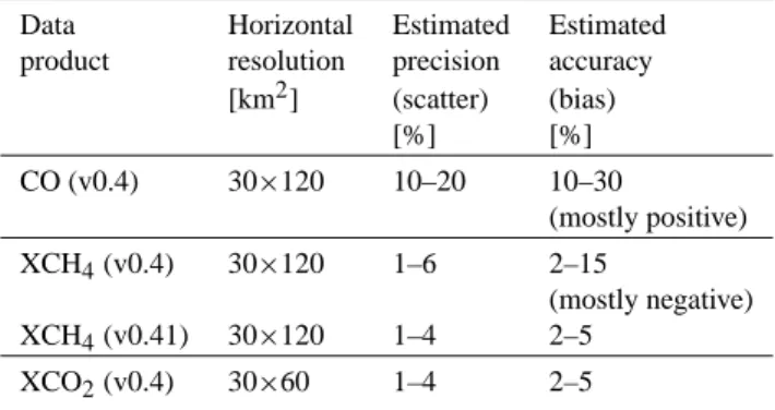
Table 1. Current estimates of precision and accuracy of the SCIAMACHY/WFM-DOAS v0.4x vertical column data products over land. The WFM-DOAS products are partially based on scaled initially retrieved columns (the scaling factors are: 0.5 for CO, 1.27 for CO2, 0.85 for O2, no scaling for methane).
Data Horizontal Estimated Estimated
product resolution precision accuracy [km2] (scatter) (bias) [%] [%] CO (v0.4) 30×120 10–20 10–30 (mostly positive) XCH4(v0.4) 30×120 1–6 2–15 (mostly negative) XCH4(v0.41) 30×120 1–4 2–5 XCO2(v0.4) 30×60 1–4 2–5
Hemisphere compared to the Northern Hemisphere. This dis-crepancy is most probably related to the difficulty of accu-rately fitting the weak CO lines covered by SCIAMACHY (see Sect. 9).
The WFM-DOAS Version 0.4 methane columns have a time dependent bias of up to about –15% related to ice build-up on the channel 8 detector. Using a simple bias correction an improved methane data product (v0.41) has been gener-ated. The comparison with model simulations shows agree-ment within a few percent (mostly within 5%). The compari-son indicates that SCIAMACHY can detect elevated methane columns resulting from emissions from surface sources such as rice fields and wetlands over India, southeast Asia and cen-tral Africa. Similar findings have been reported in Franken-berg et al. (2005c).
The (scaled) WFM-DOAS Version 0.4 CO2columns show
agreement with model simulations within a few percent (mostly within 5%). The comparison indicates that SCIA-MACHY is able to detect low columns of CO2resulting from
uptake of CO2over the Northern Hemisphere when the
veg-etation is in its main growing season. Over highly reflecting surfaces such as over the Sahara SCIAMACHY seems to sys-tematically overestimate the column averaged mixing ratio of CO2by a few percent most probably because of limitations
of the current version of the retrieval algorithm (simplified treatment of albedo and aerosol variability).
A summary of our findings from the comparisons with in-dependent data shown here and elsewhere (Buchwitz et al., 2004, 2005; Gloudemans et al., 2004; de Maziere et al., 2004; Dils et al., 2005; Sussmann et al., 2005; Sussmann and Buch-witz, 2005; Warneke et al., 2005) is given in Table 1 which shows our current best estimates of precision and accuracy of our v0.4x data products.
Our future work will focus on identifying the reasons for the observed biases and to improve the accuracy of the data