HAL Id: halshs-01677296
https://halshs.archives-ouvertes.fr/halshs-01677296
Preprint submitted on 8 Jan 2018
HAL is a multi-disciplinary open access archive for the deposit and dissemination of sci-entific research documents, whether they are pub-lished or not. The documents may come from teaching and research institutions in France or abroad, or from public or private research centers.
L’archive ouverte pluridisciplinaire HAL, est destinée au dépôt et à la diffusion de documents scientifiques de niveau recherche, publiés ou non, émanant des établissements d’enseignement et de recherche français ou étrangers, des laboratoires publics ou privés.
Tanzanian household energy choices
Johanna Choumert, Pascale Combes Motel, Leonard Le Roux
To cite this version:
Johanna Choumert, Pascale Combes Motel, Leonard Le Roux. Stacking up the ladder: A panel data analysis of Tanzanian household energy choices. 2018. �halshs-01677296�
C E N T R E D' ÉT U D E S E T D E R E C H E R C H E S S U R L E D E V E L O P P E M E N T I N T E R N A T I O N A L
SÉRIE ÉTUDES ET DOCUMENTS
Stacking up the ladder: A panel data analysis of Tanzanian
household energy choices
Johanna Choumert
Pascale Combes Motel
Leonard Le Roux
Études et Documents n° 24
December 2017
To cite this document:
Choumert J., Combes Motel P., Le Roux L. (2017) “ Stacking up the ladder: A panel data analysis
of Tanzanian household energy choices”, Études et Documents, n° 24, CERDI.
http://cerdi.org/production/show/id/1900/type_production_id/1
CERDI
65 BD. F. MITTERRAND
63000 CLERMONT FERRAND – FRANCE TEL.+33473177400
FAX +33473177428
2
The authors
Johanna Choumert
Head of Research - Economic Development Initiatives (EDI) Limited, High Wycombe, United
Kingdom/Bukoba, Tanzania.
E-mail:
j.choumert.nkolo@surveybe.com
Pascale Combes Motel
Professor - School of Economics & CERDI, University Clermont Auvergne - CNRS,
Clermont-Ferrand, France.
E-mail:
pascale.motel_combes@uca.fr
Leonard Le Roux
MCom student, School of Economics, University of Cape Town, South Africa.
E-mail:
Leonardleroux32@gmail.com
Corresponding author: Pascale Combes Motel
This work was supported by the LABEX IDGM+ (ANR-10-LABX-14-01) within the program “Investissements d’Avenir” operated by the French National Research Agency (ANR).
Études et Documents are available online at:
http://www.cerdi.org/ed
Director of Publication: Grégoire Rota-Graziosi
Editor: Catherine Araujo Bonjean
Publisher: Mariannick Cornec
ISSN: 2114 - 7957
Disclaimer:
Études et Documents is a working papers series. Working Papers are not refereed, they constitute
research in progress. Responsibility for the contents and opinions expressed in the working papers rests solely with the authors. Comments and suggestions are welcome and should be addressed to the authors.
3
Abstract
Energy-use statistics in Tanzania reflect the country’s low level of industrialization and
development. In 2016, only 16.9% of rural and 65.3% of urban inhabitants in mainland
Tanzania were connected to some form of electricity. We use a nationally representative
three-wave panel dataset (2008-2013) to contribute to the literature on household energy
use decisions in Tanzania in the context of the stacking and energy ladder hypotheses. We
firstly adopt a panel multinomial-logit approach to model the determinants of household
cooking- and lighting-fuel choices. Secondly, we focus explicitly on energy stacking
behaviour, proposing various ways of measuring what is inferred when stacking behaviour is
thought of in the context of the energy transition and presenting household level correlates
of energy stacking behaviour. Thirdly, since fuel uses have gender-differentiated impacts, we
investigate women’s bargaining power in the decision-making process of household fuel
choices. We find that whilst higher household incomes are strongly associated with a
transition towards the adoption of more modern fuels, especially lighting fuels, this
transition takes place in a context of significant fuel stacking. In Tanzania, government policy
has been aimed mostly at connecting households to the electric grid. However, the public
health, environmental and social benefits of access to modern energy sources are likely to
be diminished in a context of significant fuel stacking. Lastly, we present evidence that the
educational attainment of women in the household is an important aspect of household fuel
choices.
Keywords
Fuel choices, Intra-household bargaining, Sub-Saharan Africa.
JEL Codes
O13, Q41, N5.
Acknowledgments
We are grateful to the ANR (project REVE, ANR-14-CE05-0008) and the French Ministry of
Research for their financial support. We’d also like to thank Olivier Santoni, who compiled
the nighttime lights dataset, and Théophile Azomahou, Olivier Beaumais, Marc Jeuland,
Koen Leuveld, Aude Pommeret, François Salanié, an anonymous referee of the French
Association of Environmental and Resource Economists (FAERE) and participants of the 2017
FAERE Conference for their valuable advice. The usual disclaimers apply.
4
1 Introduction
Tanzanian energy-use statistics reflect the country’s low level of industrialization and development. According to The United Republic of Tanzania (2017), in 2016, only 16.9% of rural and 65.3% of urban inhabitants of mainland Tanzania were connected to some form of electricity. According to other sources, nationally only 2% of rural and 39% of urban inhabitants have access to electricity and only 10% of households have direct access to the national grid (UNDP, 2016).
The recent 2015 Tanzania National Energy Policy1 sets the framework to implement the new
energy policy, accounting for the United Nations’ global initiative of providing sustainable energy for all, the need for energy conservation and efficiency and the recent gas discoveries in the south-east coast of the country. The policy’s long-term objective is to improve reliable energy production and to promote productive use of energy in line with policies aimed at shaping the economic transformation of the country, where almost 30% of the population cannot meet their basic consumption needs (World Bank, 2015).
The types of fuels used by households for everyday activities, such as cooking, lighting and heating, have an important bearing on various factors influencing well-being (See Bruce et al., 2000; Dherani et al., 2008; Khandker et al., 2013; Kishore et al., 2014; Peters and Sievert, 2016; Po et al., 2011; van de Walle et al., 2017). These factors range from health outcomes and exposure to safety and financial risks to aspects of individual and collective time use. In addition, the societal relations which dictate who is exposed to the adverse effects associated with the use of traditional, ‘dirty’ fuels, such as firewood and charcoal, intimately link fuel use to the risks faced and the work carried out by women and children. Time spent collecting wood or other energy sources also represents an opportunity cost of time not spent on education or income generating activities. These immediate linkages between fuel use and well-being are also not divorced from the broader effects of a reliance on traditional fuels such as forest degradation and pollution which endanger environmental systems (Baland et al., 2010; Heltberg et al., 2000; Hofstad, 1997). For these reasons, both the short-term determinants of demand and the mechanisms of a longer-term energy transition are important to understand in order to work effectively against these adverse effects.
5
Considering the importance of the types of fuels households use, and in recognition of the various benefits associated with the adoption of modern, ‘clean’ fuels such as electricity and gas, there has been much engagement in the literature on theories of the energy transition from traditional to modern fuels.
A key early concept in the literature of the household energy transition is the energy ladder hypothesis, which views the process by which households substitute traditional fuels for modern fuels as one driven mostly by increases in income and socio-economic status (Bruce et al., 2000; Hosier and Dowd,1987; Leach, 1992; van der Kroon et al., 2013). An important aspect of this view is that it sees the energy transition as a series of largely disjointed steps in which households switch from traditional fuels, to transition fuels, and finally to clean fuels. Empirical investigations have repeatedly confirmed the importance of income in energy choices. Early studies on this topic, such as that of Hosier and Dowd (1987), also recognised that household fuel choice decisions are the result of an array of factors in addition to income levels. According to the authors, factors which influence households in ‘stepping up the ladder’ away from traditional fuels, include location, price, and infrastructure, amongst others.
In recent decades, this conception of the energy transition as one defined by fuel switching as households move up the energy ladder has been challenged by a growing body of empirical evidence that shows that households simultaneously use multiple different fuels, a characteristic described as fuel stacking (Heltberg, 2004; Masera et al., 2000; Ruiz-Mercado and Masera, 2015). The implication is that a clean-break with the use of traditional fuels is unlikely to be occurring in many developing regions today. The energy stacking hypothesis holds that as household incomes rise, the transition towards the use of modern fuels takes place in a context of the simultaneous use of various types of fuels. In this view, poorer households usually use a small variety of traditional fuels, such as firewood, animal residue and charcoal. As incomes increase, households adopt the use of modern fuels, but also continue using traditional fuels for some activities, thus ‘mixing’ various energy sources.
The household energy landscape in Tanzania is characterised by a very high prevalence of traditional fuel use, especially charcoal and firewood (The United Republic of Tanzania, 2017). Until now, to the best of our knowledge, no large scale quantitative studies have been conducted in Tanzania to empirically model the correlates of household fuel decisions using household surveys. Recent studies focus on electricity use only (Rahut et al., 2017) and charcoal expenditures only (D’Agostino et al., 2015). Considering Tanzania’s current priorities, the main goal of this paper is to develop an understanding of the nature of household energy use in
6
Tanzania in the context of the energy ladder and stacking hypotheses. More precisely, our contribution is threefold.
Firstly, we adopt a panel multinomial logit approach to model the determinants of household cooking and lighting fuel choices. To the best of our knowledge, this is the first-time household fuel choices have been explicitly modelled in this manner in Tanzania using a nationally representative panel survey. Whilst some authors, such as Mekonnen and Köhlin (2009) and Alem et al. (2016) in Ethiopia and Zhang and Hassen (2017) in urban China, have recently made use of panel data in approaching the modelling of household fuel choices, the majority of past empirical studies on this subject have been reliant on cross-sectional data. One short-coming of multinomial logit models is that they assume a series of discrete choices between the use of various fuels, thus not explicitly being able to account for stacking or fuel-mixing behaviour if mixing is not one of the categories of the dependent variables. Thus, secondly, we focus on energy stacking behaviour, proposing four ways of measuring it and deriving household correlates with these measures. Finally, since fuel uses have gender-differentiated impacts, we investigate women’s bargaining power in the decision-making process of fuel choices.
The remainder of the paper is organized as follows. Section 2 provides an overview of the energy situation in Tanzania and the data sets used for the empirical analysis. Section 3 details the empirical strategy. Thereafter, Section 4 presents the econometric results. Section 5 presents the discussion of the results.
2 Overview of the data
In this section, we firstly provide an overview of the Tanzanian National Panel Survey. Secondly, we describe how we measure intra-household bargaining. Thirdly, we detail how we proxy electricity supply and provide an overview of household energy use and fuel purchases.
2.1 Presentation of Tanzanian National Panel Survey
The compilation of the Tanzanian National Panel Survey (TZNPS) over the five-year period from October 2008 until October 20132, resulted in the production of a nationally
2 The National Panel Survey 2014-2015, Wave 4, was published in 2017. However, the sample is composed of fresh new households and is therefore not included in this study.
7
representative panel survey which provided information on a range of socio-economic indicators at the household, individual and community levels (NBS, 2014a).3
Throughout the course of the survey, the same households were tracked over three data collection rounds. Total household attrition at 4.84% (NBS, 2014b) over the entire period of the survey is sufficiently low to dispel worries of attrition-induced bias. The panel nature of the dataset and the low level of attrition are invaluable in helping to account for time-based variability, which goes unobserved in the hitherto mostly cross-sectional studies of energy use which have characterised the majority of studies on energy use in Tanzania.
The sampling design4 of the first round of the TZNPS allows for the production of
representative statistics at the national, rural/urban and major agro-ecological zone levels. The sampling design of the two subsequent rounds was based on re-contacting all households interviewed in the initial round as well as any new households which formed as a result of the splitting of original households, for example, as a result of marriage or migration. For this reason, the sample size grew from an initial sample of 3,265 households in the 2008/2009 wave to 3,924 and 5,010 households in the 2010/2011 and 2012/2013 waves, respectively (NBS, 2014b).
We chose to restrict this analysis to only those households that participated in all three waves of the survey. The reason for this is grounded in the desire to observe the factors affecting household energy choices over time, and the sample size is large enough to allow for a balanced panel dataset of 3,088 households interviewed in each of the three rounds.
For both the energy ladder and stacking model approaches, we identify in the TZNPS numerous variables, shown in Table 1 (summary statistics are provided in Table 4), which are likely to have relevance to household fuel choices. Among these are variables capturing household characteristics (what van der Kroon et al. (2013) term the “household opportunity set”), such as characteristics of the household head and the education levels and age and gender compositions of the household, and other factors relevant at the intra-household level. Secondly, household socio-economic status has been recognized in both models as a key variable
3 The dataset is publicly available and published by the World Bank as part of its Living Standards Measurement Study (LSMS) programme.
4 The unit of observation of the survey is the household and primary sampling units (PSUs) are
Enumeration Areas (EAs) from the 2002 Census. A clustered two-stage sampling design was chosen with eight households sampled randomly per PSU, and clusters were stratified along the eight administrative zones and rural areas (65%), Dar es Salaam (17.5%) and other urban areas (17.5%). The end target sample was 3,280 households in 410 EAs. The sample design is detailed in Sandefur (2009).
8
influencing the energy transition from traditional to modern fuels. In order to determine that the results are robust to different proxies of socio-economic status, we use both real per-adult-equivalent household expenditure, derived from the TZNPS expenditure questions, and a wealth index.5 Thirdly, locational aspects, such as the district and time dummy variables, are also
included.
5 It was constructed using household assets and living conditions. Steps taken in the derivation of the wealth index available from the authors upon request.
9
Table 1. Description of control variables
Variable Description Hou seh old ch ar ac ter ist ics 6 Educati on level of the househ old head
Less than primary = 1 if household head’s highest level of education is below primary school, including no schooling. Primary = 1 if household head completed primary but not junior secondary school.
Junior secondary = 1 if household head completed junior secondary but not secondary school. Secondary = 1 if household head completed secondary school but not a tertiary qualification. Tertiary = 1 if household head completed a tertiary qualification.
HH size Number of persons who normally live and eat their meals together in the household. Head age Age of household head.
Ratio of women to men Ratio of female residents to male residents.
Dependency ratio Ratio of number of members under 15 and over 65 years of age to number of members between 15 and 64 years of age. Female-headed household = 1 if household head is a woman.
Me asu res of w omen ’s ba rg aini ng p ow er Indicat or no 1
Heducouple = 1 if the husband has attained at least junior secondary education and the wife has attained less than junior secondary education (Head-powered couple) Seducouple = 1 if wife has attained at least junior secondary education and husband has attained less than junior secondary education (Spouse-powered couple) Educouple = 1 if both husband and wife have attained at least junior secondary education (Educated couple)
Neducouple = 1 if neither husband nor wife has attained junior secondary education (Undereducated couple) Indicat
or no 2 Spouse Education Years of education of the wife. Indicat
or no 3 Education Difference Years of education of the husband minus years of education of the wife. Indicat Age difference Husband’s age in years minus wife’s age in years.
6 “The word ‘household’ refers to people who live together and share income and basic needs. In other words, residents of a household share the same centre of production and consume from that centre.” (NPS, Household Questionnaire)
10 or no 4 Socio -ec on omic st at u s ind ica to
rs Log real per-adult-equivalent
expenditure
Real yearly household expenditure divided number by of adult equivalent members.7 Real yearly household expenditure is already constructed in the data and comprised of the sum of food and non-food expenditures for the household. Spatial price heterogeneity is accounted for by using Fischer food price indices. To account for inflation, we weight this by a yearly consumer price index8 based on 2010 prices.
Wealth index score Score for asset-based wealth index.
Elec/Gas stove ownership = 1 if household owns at least one electric and/or gas stove. Other stove ownership9 = 1 if household owns another type of stove.
Loca tio n al ch ar acte ris tic s
Luminosity Average level of luminosity (measured as a percentage) for the ward in which the household is located (Source: National Oceanic and Atmospheric Administration, 2008-2013) Rural household = 1 if household is classified by the TZNPS as being situated in a rural area.
Administrative District
Dummy variables Sample is divided into 7 mainland administrative districts and Zanzibar.
Fu
el
p
rices
Log Kerosene price Based on mean reported per-litre price in the EA the household is situated in. Log Firewood price Based on mean reported per-kilogramme price in the EA the household is situated in. Log electricity price Based on national energy tariffs for domestic consumption of between 50-283kWh/month. Log Charcoal price Based on mean reported per-kilogramme price in the EA the household is situated in.
7 Information on adult equivalent weights used can be found in the Survey Basic Information Document (NBS, 2014b). 8 The World Bank World Development Indicators CPI is used (World Bank, 2017).
11
2.2 Intra-household bargaining variables
Since fuel uses have gender-differentiated impacts, we also investigate women’s bargaining power in the decision-making process of household fuel choices. As stressed by Pachauri and Rao (2013) most studies on fuel choices fail to address the gender dimension. In the context of Tanzania, recent evidence shows the importance of intra-household bargaining on household decisions related to farming (Anderson et al., 2017), and more generally theoretical research highlights the relationship between intra-household distribution of power and household behaviour (Chiappori and Meghir, 2014; Doss, 2013). Moreover, there is an established literature showing that women carry out most of the house-related work in Tanzania (Budlender, 2010). In addition, in the TZNPS women report more time spent collecting firewood or other fuels than men. We can thus assume that men and women have different preferences regarding energy choices.
While measures of household welfare or locality are likely to be correlated with household cooking and lighting fuel decisions, these household-level variables do not capture intra-household dynamics which may also influence these decisions. Thus, in recognition of these societal aspects, we also include various measures of the intra-household decision making power of women. To measure women’s bargaining power, we use several proxies.10 They are presented in Table 1 (and their summary statistics
in Table 5) and include (i) a measure of the wife’s relative education level, (ii) the number of years of education of the wife, (iii) the number of years of education of the husband minus the number of years of education of the wife, and (iv) the age in years of the husband minus the age the wife. Since we are interested in women’s relative bargaining power to their husband, we only include households with a husband and a wife, and where the husband is the household head. This restricted sample has a size of 1,901 households present in each wave of the survey.
2.3 Energy variables
Below, we present the outcome variables used to test the energy ladder and energy stacking hypotheses. The TZNPS contains information on the major cooking and lighting fuels used by the household, the type and amount of four different fuels (kerosene, charcoal, electricity, and gas) purchased, and information on fuel prices in the enumeration area in which the household is located.
10 We do not include the income of the spouse due to differences in the way this information was collected across waves in the TZNPS.
12 In our approach to the energy ladder model, we adopt the classical typology of cooking fuels: (i) Modern fuels: petroleum products (e.g. kerosene and LPG) and electricity; (ii) Transition fuels: charcoal and (iii) Traditional fuels: wood fuels and agricultural waste. We classify lighting fuels similarly.
2.3.1 Variables for the energy ladder model
We identify variables in the TNZPS household questionnaires which relate to the major cooking and lighting fuels used by households based on the typology outlined above. Whilst this provides some information on the fuel-choice profile of households, it is limited by the nature of the data. Only information on the major fuels used is available in the TZNPS, whilst in its original conception, the energy ladder model concerns the exclusive use of different fuels (See Table 2).
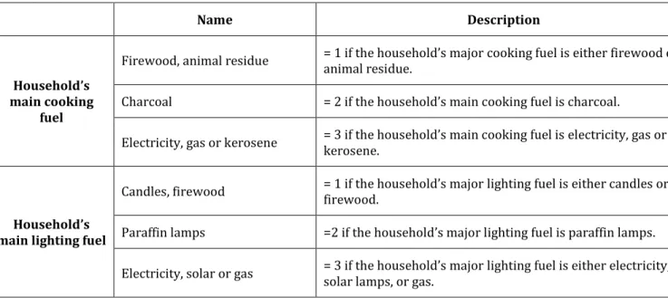
Table 2. Constructed variables for major household cooking and lighting fuels
Name Description
Household’s main cooking
fuel
Firewood, animal residue = 1 if the household’s major cooking fuel is either firewood or animal residue. Charcoal = 2 if the household’s main cooking fuel is charcoal.
Electricity, gas or kerosene = 3 if the household’s main cooking fuel is electricity, gas or kerosene.
Household’s main lighting fuel
Candles, firewood = 1 if the household’s major lighting fuel is either candles or firewood. Paraffin lamps =2 if the household’s major lighting fuel is paraffin lamps. Electricity, solar or gas = 3 if the household’s major lighting fuel is either electricity, solar lamps, or gas.
2.3.2 Variables for the energy stacking model
In order to create a sound basis for explicitly testing the energy stacking model, a key step involves creating a well-defined outcome variable which captures the qualitative and quantitative aspects of stacking behaviour. In order to do this, some theoretical decisions need to be taken.
On the one hand, an indiscriminate outcome variable in which the level of fuel stacking is determined solely by the number of different fuels a household purchased can be created. Using this, the level of fuel stacking is deemed equivalent to the number of fuels purchased. On the other hand, various continuous outcome variables can be derived, taking into account the extent to which households engage in stacking behaviour. In order not to limit the results to the type of stacking measure chosen, we present four different indicators of stacking behaviour. The four measures are outlined in Table 3, below.
13
Table 3. Various approaches to measuring fuel stacking behaviour
Name Specification Explanation
1.Simple
Stacking Number purchased: of different fuels
Where refers to the number of different fuels purchased by household i in wave t.
2.Directional
Stacking Ratio of electricity and gas in number of fuels purchased:
as above. ∑ ,
where are dummy variables taking a value of 1 if electricity and gas respectively are purchased.
3.Share
Stacking Ratio of electricity and gas expenditure in energy expenditure:
is the share of electricity and gas expenditure in total energy expenditure by household i in wave t.
4.Stacking Index
Extent of stacking given by:
∑
Stacking Index, following Andadari et al. (2014),
augmented to take into account the share of energy expenditure on clean fuels. as above.
is a dummy variable taking on a value of 1 if household i bought fuel k in period t.
Each of the four stacking measures outlined above relies on a particular conception of stacking behaviour and, whilst linked, effectively measures different types of household decisions. The Simple Stacking variable captures the most basic conception of fuel stacking by only taking into account the number of types of fuel bought, but has clear shortcomings: it does take into account the direction of stacking, i.e. which fuels are being bought, and it does not differentiate between the extent of stacking behaviour in terms of expenditure shares. There is a clear difference between a household which buys charcoal and firewood, and one which buys electricity and gas, but both households would have the same stacking score. The second, Directional Stacking variable takes into account the nature of fuel stacking by favouring stacking “up the ladder” in terms of purchases of clean fuels. The third Stacking Share variable captures the fact that households may change energy use by changing relative expenditures on various fuels. In this regard, households which dedicate more of their energy budget to modern fuels score higher on this measure. The final Stacking Index weights the number of fuels bought by the share of expenditure dedicated to clean fuels. This index has the advantage of taking into
14 account both the number of fuels bought and the share of the energy expenditure allotted to modern fuels. Arguably it would most accurately reflect stacking behaviour by having the highest score for households which purchase numerous fuels, whilst dedicating the largest share of energy expenditures towards electricity and gas.
2.3.3 Energy prices
Among the aspects of the external decision context of the household, prices households face could play an important role in the decision-making process. The community level questionnaire in the TZNPS contains price data on kerosene, charcoal, and firewood. From this data, per litre prices for kerosene and per kilogramme prices for firewood and charcoal are derived.11 Next, average prices faced
by each household are calculated by taking the mean of all prices in the EA in which the household is located. It is thus assumed that households face the average fuel prices of the community they reside in.
The TZNPS does not provide information on electricity prices. For this reason, we use national electricity tariffs. In this regard, there is no spatial variation in electricity prices, but substantial time-variation due to tariff hikes. The price information is sourced from Peng and Poudineh (2016). The State electricity provider, TANESCO, allocates five different tariff bands, dependent on the type of electricity use of the consumer. The categorisation of the consumer is based on the average voltage and consumption level of the consumer. We use the domestic use tariffs as indicators of electricity prices. Within this domestic category, there is a lifeline price which applies to usage lower than 50kWh per month, as well as a general tariff which applies to domestic use between 50-283 kWh per month. Given that a two-plate electric stove used for 3 hours a day equates to around 135kWh per month, we use the 50-283kWh tariff as an indicator of electricity prices faced by households. This tariff was subject to three adjustments throughout the panel: from 2008 until 2011 the price was 156 TZS/kWh, from 2011 to 2012 it was 195 TZH/kWh and from 2012 to 2013 it was 274 TZH/kWh.
2.4 Luminosity data as a proxy for electricity availability
In modelling household energy decisions in developing regions which are often characterised by low levels of connection to the electricity grid, access to electricity is a factor which should be taken into account. In the absence of a market for electricity (i.e. without direct household access to the electricity grid), the assumption that households face the choice whether or not to use electricity in an indirect utility maximising context is flawed. Prices are one way of getting around this factor, by assuming that
11 Potential outliers are identified using Stata’s Bacon algorithm using the 15th percentile as a threshold. However, they were only excluded from the analysis in the case that they were clearly the result of coding or capturing errors.
15 prices would reflect relative levels of supply, but in the case of electricity where prices are centrally set, this would also be inadequate.
In the absence of data on whether or not households are directly connected to the electricity grid,12
we control for electricity access using luminosity data. We make use of the DMSP-OLS Nighttime Lights data published by the U.S. National Oceanic and Atmospheric Administration (NOAA, 2008-2013).
Although there is substantial debate on whether nighttime lights data are a good proxy for economic activity in developing countries, there are several convincing arguments in favour of using this measure as a proxy for electricity consumption (Amaral et al., 2005; Chand et al., 2009; Mellander et al., 2015). Indeed, the light captured by the satellites is mainly the result of electricity-powered illumination. For instance, in a study conducted in Australia, Townsend and Bruce (2010) find a 0.93 correlation between electricity consumption and nighttime lights between 1997 and 2002. Doll and Pachauri (2010) use nighttime lights data in developing countries from 1992 to 2000 in order to investigate the capability of nighttime lights data to estimate populations without electricity access. They stress that the data tends to overestimate the population without access to electricity, as the satellite sensors may not capture low density energy usage or indoor lighting. Moreover, such data would fail to reflect situations in which households do have access to the electricity grid in an infrastructural sense, but do not use electricity. Nevertheless, this data remains extremely valuable. Hence, in the absence of publicly available information on the electricity grid in Tanzania, nighttime lights data appears to be a good and relevant proxy for electricity access.
Thus, relying on the assumption that at least some of the households in the surrounding area would have been connected to electricity grid (which would be reflected in the luminosity data), we use mean rates of luminosity at the ward13 level as a proxy for electricity access.
12 In the questionnaire, there is no specific question asking respondents whether they are connected to the grid network or not.
13 A ward is an administrative unit of the Tanzanian local governance structure that contains sub-divisions of urban and rural areas. Rural wards encompass several villages. In deriving the luminosity measure, the luminosity score of a household is given by the average level of luminosity emanating from the area covered by the ward in which it is located. Ward shape files come from the Tanzanian National Bureau of Statistics, available here:
https://goo.gl/nnoiqo.The resolution of the nighttime lights data is 30 arc seconds, which equates to roughly 1 km
16
Table 4. Pooled14 summary statistics of explanatory and explained variables (2008-2013)
Variable Mean SD Min Max
Household Characteristics
Less than primary 0.41 0.49 0 1
Primary 0.47 0.50 0 1 Junior Secondary 0.08 0.27 0 1 Secondary 0.02 0.13 0 1 Tertiary 0.01 0.10 0 1 HH Size 5.33 3.00 1 55 Head Age 47.86 15.30 16 107
Ratio of women to men 1.28 1.08 0 8 Dependency ratio 102.10 89.15 0 800 Female Headed Household 0.24 0.43 0 1
Household main cooking fuel
Firewood/Animal Residue 0.71 0.43 0 1
Charcoal 0.25 0.45 0 1
Electricity/Gas/Kerosene 0.04 0.43 0 1
Household main lighting fuel
Candles/Firewood 0.02 0.14 0 1
Paraffin Lamps 0.65 0.48 0 1
Electricity/Gas/Solar 0.24 0.42 0 1
Measures of stacking behaviour
Simple stacking 1.37 0.85 0 4 Directional stacking 0.11 0.21 0 1
Share stacking 0.12 0.25 0 1
Stacking Index 0.07 0.15 0 0.97
Socio-economic status indicators
Log per-adult-equivalent
expenditure 13.51 0.78 10.57 16.72 Wealth index score 0.00 1.97 -2.82 15.41 Elec/Gas stove ownership 0.09 0.29 0 1 Other stove ownership 0.55 0.50 0 1
Stacking Measures Simple Stacking 1.37 0.85 0 4 Directional Stacking 0.11 0.21 0 1 Share Stacking 0.12 0.25 0 1 Stacking Index 0.07 0.15 0 0.97
17
Fuel Prices & Electricity Access
Log Kerosene price 7.49 0.44 5.19 8.51 Log Firewood price 4.92 0.82 3.24 8.40 Log Electricity price 5.40 0.41 4.88 5.95 Log Charcoal price 5.77 0.67 3.74 9.52
Locational characteristics Rural household 0.67 0.47 0 1 Luminosity 9.44 19.14 0 63 Administrative zone Lake 0.10 0.29 0 1 Western 0.11 0.31 0 1 Northern 0.12 0.33 0 1 Central 0.05 0.21 0 1 Southern Highlands 0.11 0.32 0 1 Eastern 0.21 0.41 0 1 Southern 0.15 0.36 0 1 Zanzibar 0.15 0.35 0 1 N15=9,264
Source: Authors’ calculations from TZNPS (2008-2013) pooled data
Table 5. Pooled summary statistics of proxies for women’s intra-household bargaining power16
Variable Mean SD Min Max
Educouple 0.03 0.18 0 1 Seducouple 0.02 0.15 0 1 Heducouple 0.07 0.26 0 1 Neducouple 0.85 0.36 0 1 Age difference 7.80 6.85 -20 53 Education difference 0.44 2.41 -9 10 Spouse Education 7.05 2.09 0 18 N=5,70317
Source: Authors’ calculations from TZNPS (2008-2013) pooled data
15 These statistics relate to the pooled data across all three waves. Estimates for means of particular variables may be lower due to missing data.
16 A yearly breakdown of these statistics is provided in the Appendix, Annex 2.
17 These statistics relate to the pooled data of all three waves of the restricted sample of households which have a patriarchal family structure i.e. a male head and a female spouse.
18
2.5 Descriptive overview on energy use in Tanzania
On a descriptive level, many of the stylized facts concerning energy use in Tanzania are reflected in the TZNPS (2008-2013) data. High levels of traditional fuel dependency, especially for cooking, and a particularly low level of reported reliance on electricity characterise the energy situation of most households. Using the pooled data, the average reported time spent collecting firewood per household in the previous day was 40 minutes and the average time spent collecting firewood by women/female household members was four times higher than that spent by men. At the same time, there is also a significant level of spatial heterogeneity18 in dependence on both traditional lighting and cooking fuels,
with the lowest rates found near Dar es Salaam. We also find that across the country’s 26 regions there is a much higher level of variation in rates of reliance on traditional fuels for lighting purposes than for cooking. When the main cooking and lighting fuel choices of households are averaged for different segments of the per-adult-equivalent expenditure distribution in Table 6, the predominance of firewood and charcoal as the major cooking fuel types across the distribution is made clear. We see that in terms of per-adult-equivalent expenditures, of the households in the bottom 33% of the expenditure distribution, close to 96% in 2012/2013 rely on firewood as their main cooking fuel. This number consistently declines as incomes increase, as can be seen in the figures. However, it is very stable over the five-year period of the panel despite an increase in the state electricity company TANESCO’s residential users from 722 031 in 2008 to 1 014 096 in 2012 (Knoema, 2014). Of the households in the top third of the expenditure distribution in 2012/2013, 37% rely on firewood as their main cooking fuel, whilst the majority (54%) rely on charcoal. Similar results are shown for lighting fuels. The proportion of households which cite electricity, gas and solar as their main lighting fuels consistently increases as incomes increase. At the same time, the proportion of households using kerosene lamps for lighting decreases as one moves up the expenditure distribution. There is also much more time-variation in lighting fuels than in cooking fuels. In 2008-2009 45.66% of the top 33% of the expenditure distribution used electricity, gas or solar power, whilst the same figure for the 2012-2013 round is 58.17%.
Table 6. Main cooking and lighting fuels, by segment of per-adult-equivalent expenditure distribution
Main Cooking Fuel Type of Fuel 2008/2009 2010/2011 2012/2013
Poorest 33% Firewood 94.6 95.3 95.8 Charcoal 4.2 4.3 4.1 Elec/Gas/Kerosene 1.3 0.4 0.1 Total 100.0 100.0 100.0 Middle 33% Firewood 82.2 79.5 77.4
19 Charcoal 16.8 19.6 21.5 Elec/Gas/Kerosene 1.1 0.9 1.1 Total 100.0 100.0 100.0 Richest 33% Firewood 41.1 36.9 36.7 Charcoal 47.9 52.2 54.0 Elec/Gas/Kerosene 10.9 10.9 9.3 Total 100.0 100.0 100.0 N = 3,073 3,064 3,058
Main Lighting Fuel Type of Fuel 2008/2009 2010/2011 2012/2013
Poorest 33% Candles/Firewood 4.35 3.61 4.76 Kerosene Lamps 91.3 91.58 85.33 Electricity/Gas/Solar 4.35 4.81 9.92 Total 100.0 100.0 100.0 Middle 33% Candles/Firewood 1.57 1.57 1.82 Kerosene Lamps 84.07 81.17 74.64 Electricity/Gas/Solar 14.36 17.26 23.54 Total 100.0 100.0 100.0 Richest 33% Candles/Firewood 0.79 1.21 2.26 Kerosene Lamps 53.55 47.38 39.57 Electricity/Gas/Solar 45.66 51.41 58.17 Total 100.0 100.0 100.0 N19= 3,042 2,863 2,490
Source: Authors’ calculations using TZNPS (2008-2013)
From this overview, there is a clear indication that, although richer households are more likely to use modern fuels, the largest part of any transition in cooking fuels as one moves up the expenditure distribution is characterised by the tendency of richer households being more likely to use charcoal than firewood for cooking, rather than a transition towards modern fuels. This could also be explained by the fact that better-off households are likely to be urban households where firewood would not be available. On the other hand, there is much more expenditure-based variability, as well as a more substantial portion of households using modern fuels for lighting. This suggests that the rates at which households change their fuel use decisions over time and as incomes rise are different for cooking and lighting fuels. A tentative explanation of this differentiated pattern of fuel transition could be that
19 Statistics are calculated on non-missing data, which is why the number of observations varies by year and variable.
20 decisions about lighting fuels have an effect on a more diversified set of activities compared to cooking fuels. Put differently, changes in lighting fuels incur a potentially larger reallocation of resources and therefore larger welfare effects than changes in cooking fuel use. One may, therefore, expect that lighting fuel choices are more sensitive to a change in income or socio-economic status of households. In addition, the costs associated with changing towards modern cooking fuels are much higher than those associated with changing to modern lighting fuels.
Figure 1. Spending on various fuels as a ratio of total energy expenditure, by ventile of the per-adult-equivalent expenditure
N20 = 9,264. Source: Authors’ own calculations from TZNPS (2008-2013) pooled data
Using expenditure data, the information presented in Figure 1 speaks directly to the notion of fuel mixing and the energy stacking model. Households were asked whether they purchased electricity, charcoal, gas or kerosene in the preceding 30 days.21 In addition, if the answer to the question was yes,
they were asked how much they spent. In Figure 1, household energy expenditures are broken down and the average share of expenditure accruing to each of the four fuels is calculated per ventile of the distribution. We see that on average, the poorest households spend nearly all of their energy expenditure on kerosene, whilst richer households have a much more mixed portfolio of fuels. As one moves up the expenditure distribution, increasing shares of the household energy budget are allocated
20 This is the combined number of observations of households across all three waves. Expenditure information was only collected for households which purchased the given fuels. In this regard, 82% of households purchased kerosene, 31% purchased charcoal, 2% purchased gas, 21% purchased electricity.
21 Sampling rounds were structured such that the households were interviewed at the same time-period of the year in each wave.
21 to electricity and gas. However, the results echo those presented in Table 6, by demonstrating the low levels of adoption of modern fuels for most of the population. The share of energy expenditure on gas and electricity only rises above 20% for the top 10% of the income distribution scale and is under 10% for the bottom half of the income distribution scale. To put these figures into context, the data shows that the poorest households use nearly exclusively firewood and animal residue as main cooking fuels and their energy expenditure goes mostly to kerosene, which is used as the main source of lighting. Around the median of the expenditure distribution scale, households still cook mainly with firewood and animal residue, whilst more exclusively relying on kerosene as the main lighting fuel, seconded by electricity, solar or gas. The best-off households (close to the top 5% of the distribution scale) cook mainly with charcoal and use mostly modern lighting sources. The ratios of energy expenditure to total household expenditures show that most households spend between 10-20% of their total monthly expenditures on energy sources. Richer households are largely located in urban areas where due to transport costs and higher demand they are likely to have to purchase fuels such as charcoal at higher costs than in rural areas. In addition, in an urban context, the possibilities for household members collecting firewood are also likely to be more limited. For this reason, richer households are seen to spend slightly larger shares of their household budget on fuels.
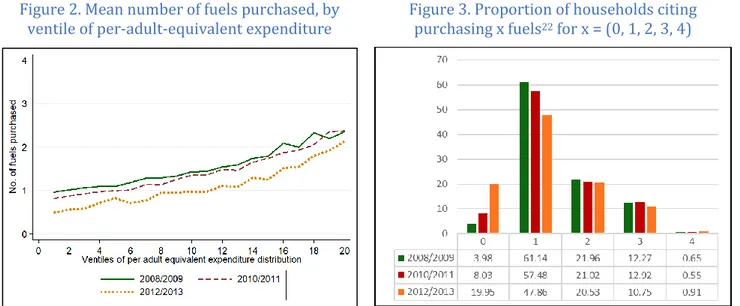
Figure 2. Mean number of fuels purchased, by
ventile of per-adult-equivalent expenditure Figure 3. Proportion of households citing purchasing x fuels22 for x = (0, 1, 2, 3, 4)
N = 9,264. Source: Authors’ own calculations from TZNPS (2008-2013) pooled data.
When the average number of fuels purchased per ventile of the per-adult-equivalent expenditure distribution is plotted in Figure 2 we see that on average richer households tend to purchase a larger number of fuels, in line with the fuel stacking hypothesis. Figure 3 shows that a large proportion (close to 30%) of households purchase more than one of the fuels surveyed. Note these statistics relate to
22 fuels purchased and not to fuels used. This is the extent of the information in the TZNPS data. The total number of fuels used may be higher.
3 Empirical strategy and econometric model
Our empirical strategy revolves around two main goals. The first is to contribute to the existing literature on the determinants of cooking and lighting fuel choices in Tanzania by adopting a multinomial logit approach. As a second goal, in recognition of the increasing relevance of the notion of fuel stacking in the literature, as well as relatively few explicit attempts to model fuel stacking using nationally representative data, we propose various ways of measuring the concept of fuel stacking and provide an analysis of the correlates of these measures.
3.1 Multinomial logit model of household fuel choices to test the energy ladder
hypothesis
When individuals are presented with the same choice successively in different time-periods, especially when that choice involves a monetary or habitual investment, they tend to make similar choices over time. There is a strong basis for this to be true, especially of cooking fuel choices. Cooking fuel choices are often associated with some investment in technology, such as stoves or hearths, as well as household-specific habits and preferences which are often persistent. These household-specific factors lead to household-specific heterogeneity, which is never fully observed.
In the fuel-choice literature, numerous authors have adopted a pooled multinomial logit approach to model fuel choices (Heltberg, 2005; Ouedraogo, 2006; Pundo and Fraser, 2006). However, this approach does not account for unobserved household heterogeneity. For these reasons, we adopt a model which takes these unobserved household effects into account.
In order to account for unobserved household heterogeneity, the two commonly used approaches are via fixed or random effects.23 Neither of these specifications imposes the assumption that repeated
household fuel choices in different time periods are independent of one another, that is, both approaches assume there is a household-specific effect but differ in the assumptions made about the nature of these effects.
We categorize both cooking and lighting fuels, respectively, into three groups according to their position in the energy spectrum, from traditional to modern fuels. In the case of cooking fuels, these
23 A general outline of random effects multinomial logit models can be found in Frees (2004, Ch.11.2) and Chen and Kuo (2001), whilst that of a fixed effects approach to multinomial logit models can be found in Pforr (2014).
23 categories are 1=firewood and animal residue, 2=charcoal and 3=electricity, gas or kerosene. In the case of lighting fuels, the categories are 1=candles and firewood, 2=paraffin lamps and 3=electricity, solar or gas. In addition, each household in the panel is observed in 3 time periods (T = 3). Thus, the observation of household i can take on a value of j = (1, 2, 3) where j refers to the category of the fuel choice.
Implicit in the model is the assumption that at any point in time, households choose those cooking or lighting fuels which maximise household utility, subject to household constraints. Thus, in a general specification taking into account unobserved household-specific effect, household i’s indirect utility associated with the choice of fuel j in time t is given by:
Where is a vector of observed explanatory variables particular to the household, and is a vector of parameters specific to fuel choice . In addition, is the unobserved household-specific effect and is an independent and identically distributed error term. In a pooled multinomial logit model, the household-specific effect is not taken into account, whilst both fixed and random effects models rely on the assumption that the explanatory variables are exogenous conditional on the household-specific term, i.e. | .
A key additional assumption specific to random effects models is that | i.e. that the unobserved household effect is independent of the explanatory variables. Under this condition and in the case where there are no omitted variables, random effects coefficient estimates are deemed to be consistent, as well as more efficient than fixed effects estimates. On the other hand, a fixed effects estimation relaxes this additional assumption and allows the household-specific effect to be correlated with the explanatory variables. Thus, a fixed effects approach allows for the derivation of consistent estimates in a case where there exist time-invariant unobserved factors which may be related to the observed explanatory variables.
The inclusion of household-specific effects implies that the probability of a household making a particular choice in one time period is subject to the same unobserved characteristics as in the other periods. This accounts for likely correlations in the error terms across repeated choices. In a multinomial logit model with unobserved household heterogeneity, the conditional probability that household i chooses fuel j in time t is thus given by:
|
( ) ∑ ( )
24 where B refers to the base outcome category. The probability is conditional on the set of household level effects and on the observable household characteristics and is estimated by way of a maximum likelihood estimator.
3.2 Stacking model
Whilst multinomial logit approaches are suited to the modelling of the energy ladder model if fuels are classed into various groups, specific studies focussed on fuel stacking need an explanatory measure capturing stacking behaviour. Some studies have attempted to explicitly model stacking behaviour using data which is not uniquely collected for that purpose. In a study in Guatemala, Heltberg (2005) creates outcome variables, capturing the stacking behaviour of households by looking at the correlates with households that use either: only wood, only LPG or LPG and charcoal for cooking. The shortcoming of this approach is that it does not take into account the extent of the stacking behaviour, nor the use of more than two fuels. In a study carried out in India, Cheng and Urpelainen (2014), use expenditure shares and information on the specific uses of different fuels, distinguishing between lighting and cooking fuels, where households use electricity and kerosene for lighting and LPG and biomass fuels in cooking. They find that whilst higher household incomes lead to decreased fuel stacking for lighting, the same is not true for cooking. In an impact evaluation study of a government LPG promotion programme, Andadari et al. (2014) create an index of fuel stacking by weighting the number of fuels used by the total number possible in the dataset. This is useful in a descriptive sense but does not capture the direction of fuel stacking, i.e. households which perform higher on the index do not necessarily stack ‘up the ladder’ by increasing modern fuel use.
4 Results
4.1 Multinomial logit regression results
Both household cooking and lighting decisions are modelled using a multinomial logit approach. The full regression output using pooled, fixed effects and random effects specifications, as well as the constructed wealth index as an alternative measure of socio-economic status, are displayed in Annex 4 and 5. Below, in Table 7 and Table 8, the average marginal effects of the random effects regressions are displayed due to the omission of time-invariant household variables, such as location and educational attainment, in a fixed effects estimation. The marginal effects we display allow us to illustrate how these factors correlate with fuel choices. A Small-Hsiao test rejects the null hypothesis of a violation of the independence of irrelevant alternatives assumption across all eliminated categories in the case of lighting fuels, and consistently for two of the eliminated categories for cooking fuels, and inconsistently
25 for the third. There has, however, been extensive engagement on the reliability of these types of tests which cast doubt on their usefulness for empirical work (Cheng and Long, 2007; Fry and Harris, 1998; Fry and Harris, 1996).
Table 7. Average marginal effects from random effects regression results: cooking fuels
Firewood/Animal Res. Charcoal Electricity/ Kerosene/Gas
dy/dx Std. Err. dy/dx Std. Err. dy/dx Std. Err.
Log per. ad. eq. expenditure -0.095*** 0.009 0.082*** 0.010 0.013*** 0.005
Luminosity -0.003*** 0.000 0.002*** 0.000 0.000** 0.000 Rural Household 0.175*** 0.017 -0.162*** 0.018 -0.013** 0.006 Primary -0.040*** 0.011 0.023* 0.013 0.017** 0.008 Junior Secondary -0.121*** 0.024 0.087*** 0.027 0.034** 0.016 Secondary -0.122** 0.048 0.099** 0.050 0.023 0.021 Tertiary -0.130 0.087 0.036 0.082 0.095** 0.043 Female Headed HH -0.028** 0.012 0.035*** 0.013 -0.008 0.005 HH Size 0.002 0.002 0.001 0.002 -0.003** 0.001
Ratio of Women to Men -0.001 0.004 0.005 0.004 -0.004 0.002
HH Head age 0.001*** 0.000 -0.001** 0.000 0.000 0.000
Elec/Gas stove -0.066*** 0.022 0.025 0.022 0.041*** 0.011
Other Stove -0.131*** 0.013 0.147*** 0.014 -0.016** 0.008
Log Kerosene Price -0.012 0.026 0.000 0.028 0.013 0.012
Log Firewood Price 0.005 0.008 -0.005 0.009 -0.001 0.003
Log Charcoal Price -0.003 0.012 0.002 0.012 0.001 0.005
Log Electricity Price -0.009 0.046 0.044 0.048 -0.034* 0.019
Admin. District Dummy Variables YES YES YES
Wave Dummy Variables YES YES YES
N= 3,575
* p<0.10, ** p<0.05, *** p<0.010. These marginal effects estimates are calculated from random effects multinomial logit results presented fully in Annex 4. In addition, marginal effects calculated at various points of the log per-adult equivalent expenditure distribution function are presented in Annex 6.
The average marginal effects estimates for the random effects cooking fuel regression show that per-adult-equivalent expenditure is significantly correlated with household fuel choices and that households with higher levels of per-adult-equivalent expenditures on average are less likely to use biomass fuels as their main cooking fuel, but more likely to use charcoal than electricity. This result is not so puzzling, given the high level of charcoal use and low levels of electricity use for cooking in the country.
In addition, we see that the relationship between luminosity rates and major cooking fuel choices is very weak and the marginal effects coefficient close to zero. This alludes to the likelihood that ceteris
26 paribus, access to electricity does not necessarily lead to the exclusive adoption of modern fuels. This could be explained by the positive externalities of having neighbours or businesses with access to electricity or living in a town with street lights. Following van de Walle et al. (2017), there is a distinction between the internal effects of a household’s electrification and the external effects of village electrification which can lead to different types of spillovers, hence of behaviour in terms of energy choices.
Rural households are substantially less likely to use clean fuels as their major cooking fuel than urban households. We see that rural households are 17% more likely to use firewood/animal residue, 16% less likely to use charcoal and 1% less likely than urban households to use clean fuels as their main cooking fuel. Similarly, households in areas where luminosity scores are higher are less likely to use firewood and animal residue. We also see that households which have access to electric or gas stoves are significantly more likely than those which do not to use clean fuels and less likely to use biofuels.24
Female-headed households are more likely than non-female-headed households to rely on charcoal and less likely to rely on biofuels as a main cooking fuel source.
The level of education of the household head is positively associated with a transition towards the use of modern fuels. In particular, we see that households in which the head has obtained tertiary are 9% more likely to use clean fuels as their main cooking fuels than households without primary education (the base case). When looking at the price effects, it is surprising to see that only the electricity price is weakly significant (at the 10% level). The marginal effects illustrate that a 10% increase in the electricity price is associated with a 0.3% decrease in the likelihood of using modern fuels.
Table 8. Average marginal effects from random effects regression results: Lighting fuels
Candles/ Firewood Lamp Oil (Kerosene/ Paraffin) Electricity/ Gas/ Solar
dy/dx Std. Err. dy/dx Std. Err. dy/dx Std. Err.
Log per.ad.eq. Expenditure -0.006** 0.003 -0.088*** 0.009 0.094*** 0.009
Luminosity 0.000** 0.000 -0.003*** 0.000 0.003*** 0.000
Rural Household 0.000 0.002 0.122*** 0.014 -0.121*** 0.014
Primary -0.002 0.002 -0.061*** 0.011 0.064*** 0.011
Junior Secondary -0.001 0.003 -0.262*** 0.033 0.264*** 0.035
24 In their systematic review on who adopts improved fuels and cookstoves, Lewis and Pattanayak (2012) find that cookstoves programmes have low rates of adoption in developing economies, and this despite the triple dividends (household health, local environmental quality, and regional climate benefits) that could result from the use of improved cook stoves and clean fuels. Unfortunately, in our dataset, we cannot make a precise distinction between different types of cook stoves. Most household surveys do not provide such detailed information. This would deserve further attention in the context of Tanzania.
27
Secondary -0.004** 0.002 -0.384*** 0.090 0.388*** 0.090
Tertiary -0.004** 0.002 -0.331*** 0.124 0.334*** 0.124
Female Headed HH -0.002 0.001 0.032*** 0.012 -0.031** 0.012
HH Size -0.001 0.000 -0.004** 0.002 0.005*** 0.002
Ratio of Women to Men 0.000 0.000 -0.011* 0.004 0.011** 0.004
HH Head Age 0.000 0.000 -0.001*** 0.000 0.001*** 0.000
Log Kerosene Price 0.001 0.004 -0.089*** 0.024 0.087*** 0.024
Log Firewood Price -0.003* 0.002 -0.006 0.007 0.009 0.007
Log Electricity Price 0.017* 0.010 -0.015 0.046 -0.002 0.045
Admin. District Dummy Variables YES YES YES
Wave Dummy Variables YES YES YES
N = 5,007
* p<0.10, ** p<0.05, *** p<0.010. These marginal effects estimates are calculated from random effects multinomial logit results presented fully in Annex 5. In addition, Marginal effects calculated at various points of the log per-adult equivalent expenditure distribution function are presented in Annex 6.
The marginal effects estimates for the categorical lighting fuel variable in Table 8 also show that per-adult-equivalent expenditure is positively and significantly correlated with the use of modern fuels. In the case of lighting fuels, the effect of increases in per-adult-equivalent expenditure is largest for modern fuels. All else equal, rural households are also less likely than urban households to use more modern lighting sources. In addition, as expected, households in areas with higher rates of luminosity have a higher probability of mainly using modern lighting fuels.
Female-headed households are less likely to use modern fuels than households headed by men; however, households with a higher ratio of women to men are more likely to use mainly modern lighting fuels. In addition, larger households are more likely to use modern fuels, perhaps alluding to the relative cost of modern fuels, which can be more easily incurred by larger households. The results in Table 6 also show that a 10% increase in the kerosene price results in a 0.9% decrease in the likelihood of using lamp oil as a fuel source for lighting and an almost equivalent 0.9% increase in the likelihood of using modern fuels, suggesting that households easily switch between paraffin lamps and modern lights, such as solar or electric lamps.
We also see that marginal changes in expenditure have larger effects on the probabilities of households’ main cooking fuel choices as one moves up the expenditure distribution25. We observe that
at the mean of the per-adult-equivalent expenditure, a 10% increase in per-adult-equivalent expenditure results in a roughly 11% decrease in the probability of using mainly firewood and animal residue, a 10% increase in the probability of using charcoal and a 1% increase in the probability of using modern fuels. Across the expenditure distribution, the probability of using charcoal associated
25 This relates to marginal affects estimates presented in Annex 6.
28 with an increase in expenditure is always higher than the probability of using modern fuels. For lighting fuels, we see that at the mean of the per-adult-equivalent expenditure distribution, a 10% increase in per-adult-equivalent expenditure results in a 1% decrease in the probability of using firewood and candles as a main lighting fuel, a 10% decrease in the probability of using lamp oil and a 9% increase in the probability of using modern lighting fuels. Thus, when focussing on the relative sizes of the marginal effects, increases in income are always associated with an increase in the probability of using modern fuels and a decrease in the probability of using lamp oil, firewood, and candles.
4.2 Household fuel stacking results
Table 9 displays the results of panel regressions of the correlates of fuel stacking using the Stacking Index presented in Table 3 as the dependent variable and using three different estimators. We display results of the random effects generalised least squares (GLS) and maximum likelihood (ML) estimators as well as fixed effects results. As a robustness test, GLS regressions using each of the other stacking measures are presented in the Appendix, Annex 7, showing that the results are not generally dependent on the choice of the stacking measures proposed here.
Table 9. Fuel stacking panel regressions: Stacking Index as dependent variable
(1) (2) (3)
Random Effects GLS Random Effects ML Fixed Effects
Log per.ad.eq.expenditure 0.0343*** 0.0346*** 0.00897*** (0.00) (0.00) (0.00) Luminosity 0.00217*** 0.00216*** 0.00143*** (0.00) (0.00) (0.00) Rural Households -0.0269*** -0.0271*** (0.00) (0.00) Primary 0.00803** 0.00796** (0.00) (0.00) Junior Secondary 0.0748*** 0.0751*** (0.01) (0.01) Secondary 0.117*** 0.117*** (0.01) (0.01) Tertiary 0.192*** 0.193*** (0.02) (0.02) Female Head HH -0.00674 -0.00675 -0.00555 (0.00) (0.00) (0.01) Household size 0.00192*** 0.00195*** -0.000509 (0.00) (0.00) (0.00)
Ratio of women to men 0.000724 0.000755 -0.00217
(0.00) (0.00) (0.00)
29
(0.01) (0.01)
Log Electricity Price 0.00318 0.00299
(0.02) (0.02)
Log Firewood Price -0.00680** -0.00681**
(0.00) (0.00)
Log Charcoal Price 0.00707* 0.00709*
(0.00) (0.00)
Constant -0.617*** -0.621*** -0.0600
(0.11) (0.11) (0.04)
Admin. District Dummy Variables YES YES NO
Wave Dummy Variables YES YES YES
sigma_u constant 0.0830*** (0.00) sigma_e constant 0.0704*** (0.00) Overall R-Squared 0.41 0.23 N 4936 4936 7288
* p<0.10, ** p<0.05, *** p<0.010. Standard errors in parentheses.
Across all three specifications in Table 9, we find significant correlations of fuel stacking behaviour as measured by the Stacking Index and by increases in per-adult-equivalent expenditure. Using the other measures of fuel stacking presented in Annex 7, we find the same result, supporting the fuel stacking hypothesis. We find that a 10% increase in per-adult-equivalent expenditure on average is associated with an increase of between 0.001 and 0.0035 on the Stacking Index score. Similar positive and significant effects for the luminosity coefficients suggest that household access to electricity is not necessarily a determinant of a full transition to the exclusive use of modern fuels. The results also show significant urban-rural disparities in levels of fuel stacking, with rural households scoring on average around 0.03 less on the Stacking Index than urban households, ceteris paribus.
Higher education levels are also correlated with higher levels of fuel stacking. The size of the coefficients on the education dummy variables increase as the level of education increases. Thus, the largest coefficient of all the education dummy variables is on tertiary education, signifying that households in which the household head is more educated are more likely to score higher on the Stacking Index. Of the price measures, we see that wood and kerosene price effects are significant at the 5% level.
Aside from the nature of the household energy transition, there has been a debate on why households choose to use a mixture of different fuels. It has been highlighted that fuel choice decisions are explained by numerous, often interlinked factors. In particular, the influence of cultural preferences has emerged in the literature. Ruiz-Mercado and Masera (2015) argue that in most cases, modern fuels