Designing Hardware for Machine Learning: The Important Role Played by Circuit Designers

Designing Hardware for Machine Learning: The

Important Role Played by Circuit Designers

The MIT Faculty has made this article openly available.

Please share

how this access benefits you. Your story matters.

Citation

Sze, Vivienne. "Designing Hardware for Machine Learning: The

Important Role Played by Circuit Designers." IEEE Solid-State

Circuits Magazine 9, 4 (November 2017): 46-54 © 2017 IEEE

As Published

http://dx.doi.org/10.1109/mssc.2017.2745798

Publisher

Institute of Electrical and Electronics Engineers (IEEE)

Version

Author's final manuscript

Citable link

https://hdl.handle.net/1721.1/129802

Terms of Use

Creative Commons Attribution-Noncommercial-Share Alike

Designing Hardware for Machine Learning

Vivienne Sze

Abstract—Machine learning is becoming increasingly impor-tant in the era of big data. It enables us to extract meaningful information from the overwhelming amount of data that is being generated and collected every day. This information can be used to analyze and understand the data to identify trends (e.g., surveil-lance, portable/wearable electronics); or to take immediate action (e.g., robotics/drones, self-driving cars, smart Internet of Things). In many applications, embedded processing near the sensor is preferred over the cloud due to privacy or latency concerns, or limitations in the communication bandwidth. However, sensor devices often have stringent constraints on energy consumption and cost in addition to throughput and accuracy requirements. Circuit designers can play an important role in addressing these challenges by developing energy-efficient platforms to perform the necessary processing for machine learning. In this tutorial, we will give a short overview of the key concepts in machine learning, discuss its challenges particularly in the embedded space, and highlight various opportunities where circuit designers can help to address these challenges.

I. INTRODUCTION

Machine learningis needed to extract meaningful, and ideally actionable, information from the overwhelming amount of data that is being generated and collected every day. Given the sheer volume of data, the high energy cost of communication and the often limited communication bandwidth, there is an increasing need to perform the analysis locally near the sensor rather than sending the raw data to the cloud. Enabling machine learning at the edge also addresses important concerns related to privacy, latency and security. Accordingly, embedded machine learning has shown to be beneficial for many applications in the multimedia and medical fields.

For instance, computer vision is a form of machine learning that extracts information from images and videos, which are arguably the biggest of the big data as they account for over 70% of today’s Internet traffic [1]. In many applications (e.g., measuring wait times in stores, traffic patterns), it is desirable to extract the meaningful information from the video at the image sensor rather than in the cloud to reduce the communication cost. For other applications such as autonomous vehicles, drone navigation and robotics, local processing is desired since the latency and security risk of relying on the cloud are too high. However, video involves a large amount of data, which is computationally expensive to process; thus, low cost hardware to analyze video is challenging yet critical to enabling these applications. While there is a wide range of computer vision tasks [2], in this article, we will focus on image classification as a driving example, where the task is to determine the class of objects in the image (Fig. 1).

Another important application is speech recognition, which enables us to seamlessly interact with electronic devices, such as smartphones. Speech recognition is the first step before

Dog (0.7) Cat (0.1) Bike (0.02) Car (0.02) Plane (0.02) House (0.04) Machine Learning (Inference)

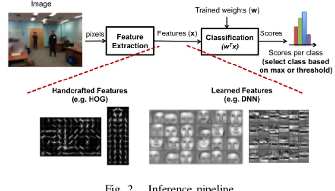
Fig. 1. Example of an image classification task. The machine learning platform takes in an image and outputs the confidence scores for a predefined set of classes. Feature Extraction Classification (wTx) Handcrafted Features (e.g. HOG) Learned Features (e.g. DNN) pixels Features (x) Trained weights (w) Image Scores Scores per class (select class based on max or threshold)

Fig. 2. Inference pipeline.

many other tasks such as machine translation, natural language processing, etc. Low power hardware for speech recognition is explored in [3, 4].

In the medical field, there is a clinical need to collect long-term data to help detect/diagnose various diseases or monitor treatment. For instance, constant monitoring of ECG or EEG signals can identify cardiovascular diseases or detect the onset of a seizure for epilepsy patients, respectively. In many cases, these devices are either wearable or implantable, and thus the energy consumption must be kept to a minimum. The use of embedded machine learning to extract meaningful physiological signals and process them locally is explored in [5, 6].

II. MACHINELEARNINGBASICS

Machine learning is a form of artificial intelligence (AI) that can perform a task without being specifically programmed. Instead, it learns from previous examples of the given task during a process called training. After learning, the task is performed on new data through a process called inference. Machine learning is particularly useful for applications where the data is difficult to model analytically.

A typical machine learning pipeline for inference can be broken down into two steps as shown in Fig. 2: Feature Extraction and Classification. Approaches such as deep neural networks (DNN) blur the distinction between these steps.

A. Feature Extraction

Feature extraction is used to transform the raw data into meaningful representations for the given task. Traditionally, feature extraction was designed through a hand-crafted process by experts in the field. For instance, it was observed that humans are sensitive to edges (i.e., gradients) in an image. As a result, many well-known computer vision algorithms use image gradient-based features such as Histogram of Oriented Gradients (HOG) [7] and Scale Invariant Feature Transform (SIFT) [8]. The challenge in designing these features is to make them robust to variations in illumination and noise. B. Classification

The output of feature extraction is represented by a vector (x in Fig. 2), which is mapped to a score of confidence using a classifier. Depending on the application, the score is either compared to a threshold to determine if an object is present, or compared to the other scores to determine the object class. Techniques for classification include linear methods such as support vector machine (SVM) [9] and Softmax, and non-linear methods such as kernel-SVM [9] and Adaboost [10]. Many of these classifiers compute the score using a dot product of the features (~x) and a set of weights ( ~w) (i.e.,P

iwixi). As

a result, machine learning hardware research tends to focus on reducing the cost of a multiply and accumulate (MAC) operation.

Training involves learning these weights from a dataset. Inference involves performing a given task using the trained weights. In most cases, training is done in the cloud, while inference can happen in the cloud or locally on a device near the sensor. In latter case, the trained weights are downloaded from the cloud and stored on the device. Thus, the device needs to be programmable in order to support a reasonable range of tasks.

C. Deep Neural Networks (DNN)

Rather than using hand-crafted features, the features can be directly learned from the data, similar to the weights in the classifier, such that the entire system is trained end-to-end. These learned features are used in a popular form of machine learning called deep neural networks (DNN), also known as deep learning [11]. DNNs deliver higher accuracy than hand-crafted features, sometimes even better than human level accuracy, on a variety of tasks by mapping inputs to a high-dimensional representation; however, it comes at the cost of high computational complexity, resulting in orders of magnitude higher energy consumption than hand-crafted approaches [12].

There are many forms of DNN (e.g., convolutional neural networks, recurrent neural networks, etc.). For computer vision applications, DNNs are often composed of multiple convolu-tional (CONV) layers [13] as shown in Fig. 3; each CONV layer involves the application of multiple high-dimensional filters to the incoming data. With each layer, a higher-level abstraction of the input data, called a feature map, is extracted that preserves essential yet unique information. Modern DNNs

Modern DNNs: 5 – 1000 Layers Classes FC Layer CONV Layer Low-Level

Features CONV _Layer

High-Level Features … 1 – 3 Layers convolu'on non-linearity × normaliza'on pooling

Fig. 3. Deep Neural Networks are composed of several convolutional layers followed by fully connected layers.

TABLE I

SUMMARY OF POPULARDNNS[16, 18–21]. ACCURACY MEASURED BASED ONTOP-5ERROR ONIMAGENET[22].

Metrics LeNet AlexNet VGG-16 GoogLeNet ResNet

5 16 (v1) 50 Accuracy n/a 16.4 7.4 6.7 5.3 CONV Layers 2 5 16 21 49 Weights 2.6k 2.3M 14.7M 6.0M 23.5M MACs 283k 666M 15.3G 1.43G 3.86G FC Layers 2 3 3 1 1 Weights 58k 58.6M 124M 1M 2M MACs 58k 58.6M 124M 1M 2M Total Weights 60k 61M 138M 7M 25.5M Total MACs 341k 724M 15.5G 1.43G 3.9G

are able to achieve superior performance by employing a very deephierarchy of layers, on the order of tens to hundreds.

The output of the final CONV layer is typically processed by fully-connected (FC) layers for classification. In FC layers, the filter and input feature map are the same size, so that there is a unique weight for each input feature value. In between CONV and FC layers, additional functions can be added, such as pooling and normalization [14]. In addition, a non-linear function, such as a rectified linear unit (ReLU) [15], is applied after each CONV and FC layer. Overall, convolutions still account for over 90% of the run-time and energy consumption in modern DNNs for computer vision.

Table I compares modern DNNs, with a popular neural net from the 1990s, LeNet-5 [16]. Today’s DNNs use more layers (i.e., deeper) and are several orders of magnitude larger in terms of compute and storage. A more detailed discussion on DNNs can be found in [17].

D. Impact of Difficulty of Task on Complexity

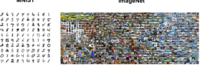
The difficulty of the task must be considered when comparing different hardware platforms for machine learning, as the size of the classifier or network (i.e., number of weights) and the number of MACs tend to be larger for more difficult tasks and thus require more energy. For instance, the task of classifying handwritten digits from the MNIST dataset [23] is much simpler than classifying an object into one of a 1000 classes in the ImageNet dataset [22](Fig. 4). Accordingly, LeNet-5, which is designed for digit classification, requires much

MNIST ImageNet

Fig. 4. MNIST (10 classes, 60k training, 10k testing) [23] vs. ImageNet (1000 classes, 1.3M training, 100k testing) [22] dataset.

less storage and compute than the larger DNNs in Table I, which are designed for the 1000-class image classification task. Thus, hardware platforms should only be compared when performing machine learning tasks of similar difficulty and accuracy; ideally, the same task with the same accuracy.

III. CHALLENGES

The key metrics for embedded machine learning are accuracy, energy consumption, throughput, and cost. The challenge is to address all these requirements concurrently.

As previously discussed, the accuracy of the machine learning algorithm should be measured for a well-defined task on a sufficiently large dataset (e.g., ImageNet).

Energy consumption is often dominated by data movement as memory access consumes significantly more energy than computation [24]. This is particularly challenging for machine learning as the high dimensional representation and filters increase the amount of data generated, and the programmability needed to support different applications, tasks and networks means that the weights also need to be read and stored. In this article, we will discuss various methods that reduce data movement to minimize energy consumption.

The throughput is dictated by the amount of computation, which also increases with the dimensionality of the data. In this article, we will discuss various transforms that can be applied to the data to reduce the number of required operations.

The cost is dictated by the amount of storage required on the chip. In this article, we will discuss various methods to reduce storage costs such that the area of the chip is reduced, while maintaining low off-chip memory bandwidth.

Currently, state-of-the-art DNNs consume orders of magni-tude higher energy than other forms of embedded processing (e.g., video compression) [12]. We must exploit opportunities at multiple levels of hardware design to address all these challenges and close this energy gap.

IV. OPPORTUNITIES INARCHITECTURES

The MAC operations in both the feature extraction (CONV layers in a DNN) and classification (for both DNN and hand-crafted features) can be easily parallelized. Two common highly-parallel compute paradigms that can be used are shown in Fig. 5.

A. CPU and GPU Platforms

CPUs and GPUs use temporal architectures such as SIMD or SIMT to perform the MACs in parallel. All the arithmetic logic

Temporal Architecture (SIMD/SIMT) Spatial Architecture (Dataflow Processing) Register File Memory Hierarchy ALU ALU ALU ALU ALU ALU ALU ALU ALU ALU ALU ALU ALU ALU ALU ALU Control Memory Hierarchy

ALU ALU ALU ALU

ALU ALU ALU ALU

ALU ALU ALU ALU

ALU ALU ALU ALU

Fig. 5. Highly-parallel compute paradigms with multiple arithmetic logic units (ALU).

units (ALUs) share the same control and memory (register file). On these platforms, all classifications are represented by a matrix multiplication. The CONV layer in a DNN can also be mapped to a matrix multiplication using the Toeplitz matrix. Software libraries that optimize for matrix multiplications can be used to accelerate processing on CPUs (e.g., OpenBLAS, Intel MKL, etc.) and GPUs (e.g., cuBLAS, cuDNN, etc.). The matrix multiplications can be further sped up by applying transforms such as Fast Fourier Transform (FFT) [25, 26] and Winograd [27] to the data to reduce the number of multiplications.

B. Specialized Hardware

Specialized hardware provides an opportunity to optimize the data movement (i.e., dataflow) in order to minimize accesses from the expensive levels of the memory hierarchy and maximize data reuse at the low-cost levels of the memory hierarchy. Fig. 6 shows the memory hierarchy of the spatial architecture in Fig. 5, where each ALU processing element (PE) has a local memory (register file) on the order of several kB and a shared memory (global buffer) on the order of several hundred kB. The global buffer communicates with the off-chip memory (e.g., DRAM). Data movement is allowed between the PEs using an on-chip network (NoC) to reduce accesses to the global buffer and the off-chip memory.

The dataflows of all three types of data (feature map, filter weights and partial sums) affect energy consumption. Various dataflows have been demonstrated in recent works [28–39], which differ in terms of the type of data that moves and the type of data that remains stationary in the register file [40]. The row stationary dataflow, which considers the energy consumption of all three data types, reduces the energy consumption by 1.4× to 2.5× compared to the other dataflows for the CONV layers [41].

V. OPPORTUNITIES INJOINTALGORITHM ANDHARDWARE DESIGN

The machine learning algorithms can be modified to make them more hardware-friendly by reducing computation, data

DRAM Global _Buffer

PE PE PE

ALU fetch data to run a MAC here

ALU

Buffer ALU

RF ALU

Normalized Energy Cost

200× 6× PE ALU 2× 1× 1× (Reference) DRAM ALU 0.5 – 1.0 kB 100 – 500 kB NoC: 200 – 1000 PEs

Fig. 6. Memory hierarchy and data movement energy for a spatial architecture [41].

movement and storage requirements, while maintaining accu-racy.

A. Reduce Precision

GPUs and CPUs commonly use 32-bit floating-point as the default representation. For inference, it is possible to use fixed-point with reduced bitwidth for energy and area savings, and increased throughput, without affecting accuracy.

For instance, for object detection using hand-crafted HOG features, only 11-bits are required per feature vector and only 5-bits are required per SVM weight [42]. For DNN inference, recent commercial hardware uses 8-bit integer operations [43]. Custom hardware can be used to exploit the fact that the minimum bitwidths varies per layer for energy savings [44] or increased throughput [45]. With more significant changes to the network, it is possible to reduce the bitwidth of DNNs to 1-bit at the cost of reduced accuracy [46, 47].

B. Sparsity

Increasing sparsity in the data reduces storage and com-putation cost. For SVM classification, the weights can be projected onto a basis such that the resulting weights are sparse for a 2× reduction in number of multiplications [42]. For feature extraction, the input image can be made sparse by pre-processing for a 24% reduction in power consumption [48]. For DNNs, the number of MACs and weights can be reduced by removing weights through a process called pruning. This was first explored in [49] where weights with minimal impact on the output were removed. In [50], pruning is applied to modern DNNs by removing small weights. However, removing weights does not necessarily lead to lower energy. Accordingly, in [51] weights are removed based on an energy-model [52] to directly minimize energy consumption.

Specialized hardware in [42, 53–55] exploits sparse weights for increased speed or reduced energy consumption. In Eye-riss [53], the processing elements are designed to skip reads and MACs when the inputs are zero, resulting in a 45% energy reduction. In [42], specialized hardware is designed to avoid computation and storage of zero-valued weights, which reduces the energy and storage cost by 43% and 34%, respectively.

0.02 0.04 0.06 WLDAC Code

Δ

V

(V

)

Ideal transfer curve

Nominal transfer curve Standard Deviation

(from Monte Carlo simulations)

IBC WLDAC code

ΔVBL

(a) Multiplication performed by bit-cell (Figure from [57]) V₁ G₁ I₁ = V₁×G₁ V₂ G₂ I₂ = V₂×G₂ I = I₁ + I₂ = V₁×G₁ + V₂×G₂ (b) Giis conductance of resistive

memory (Figure from [58]) Fig. 7. Analog computation by (a) SRAM bit-cell and (b) non-volatile resistive memory.

C. Compression

Lightweight compression can be applied to exploit data statistics (e.g., sparsity) to further reduce data movement and storage cost. Lossless compression can reduce the transfer of data on and off chip by around 2× as shown in [5, 44, 55]. Lossy compression such as vector quantization can also be used on feature vectors [42] and weights [3, 6, 56] such that they can be stored on-chip at low cost. When lossy compression is used, it is also important to evaluate the impact on accuracy.

VI. OPPORTUNITIES INMIXED-SIGNALCIRCUITS Mixed-signal circuit design can be used to address the data movement between the memory and processing element (PE), and also the sensor and PE. However, circuit non-idealities should be factored into the algorithm design, for instance, by reducing precision as discussed in Section V. In addition, since the training often occurs in the digital domain, the ADC and DAC overhead should also be accounted for when evaluating the system.

While spatial architectures bring the memory closer to the computation (i.e., into the PE), there have also been efforts to integrate the computation into the memory itself. For instance, in [57] the classification is embedded in the SRAM (Fig. 7(a)), where the bit-cell current is effectively a product of the value of the 5-bit feature vector (WLDAC) that drives the word line (WL), and the value of the binary weight stored in the bit-cell. The currents from bit-cells in the column are added together to discharge the bitline (BL) by ∆VBL. This approach gives

12× energy savings over reading the 1-bit weights from the SRAM.

Recent work has also explored the use of mixed-signal cir-cuits to reduce the computation cost of the MAC. It was shown in [59] that performing the MAC using switched capacitors can potentially be more energy-efficient than digital circuits at low bitwidths despite ADC and DAC overhead. In [60, 61], the matrix multiplication (with bitwidths ≤ 8-bits) is integrated

into the ADC; this also moves the computation closer to the sensor and reduces the number of ADC conversions by 21×. To further reduce the data movement from the sensor, [62] proposed performing the entire CONV layer in the analog domain at the sensor. Similarly, in [63], the entire HOG feature is computed in the analog domain to reduce the sensor bandwidth by 96.5%.

VII. OPPORTUNITIES INADVANCEDTECHNOLOGIES Advanced technologies can also be used to reduce data movement by moving the processing and memory closer together. For instance, embedded DRAM (eDRAM) and Hyper Memory Cube (HMC) are explored in [39] and [64], respectively, to reduce the energy access cost of the weights in DNN. The multiplication can also be directly integrated into advanced non-volatile memories [65] by using them as resistive elements (Fig. 7(b)). Specifically, the multiplications are performed where the conductance is the weight, the voltage is the input, and the current is the output; the addition is done by summing the current using Kirchhoff’s current law. Similar to the mixed-signal circuits, the precision is limited, and the ADC and DAC overhead must be considered in the overall cost. DNN processing using memristors is demonstrated in [58, 66], where the bitwidth of the memristors is restricted to 2 to 4 bits.

The computation can also be embedded into the sensors. For instance, an Angle Sensitive Pixels sensor can be used to compute the gradient of the image input, which along with compression, reduces the sensor bandwidth by 10× [67]. Such a sensor can also reduce the computation and energy consumption of the subsequent processing engine [48, 68].

VIII. SUMMARY

Machine learning is an important area of research with many promising applications and opportunities for innovation at various levels of hardware design. The challenge is to balance the accuracy, energy, throughput and cost requirements.

Since data movement dominates energy consumption, the primary focus of recent research has been to reduce the data movement while maintaining accuracy, throughput and cost. This means selecting architectures with favorable memory hierarchies like a spatial array, and developing dataflows that increase data reuse at the low-cost levels of the memory hierarchy. With joint design of algorithm and hardware, reduced bitwidth precision, increased sparsity and compression are used to further reduce the data movement requirements. With mixed-signal circuit design and advanced technologies, computation is moved closer to the source by embedding computation near or within the sensor and in the memories.

Finally, designers should also consider the interactions between the different levels. For instance, reducing the bitwidth through hardware-friendly algorithm design enables reduced precision processing with mixed-signal circuits and non-volatile memories. Reducing the cost of memory access with advanced technologies could also result in more energy-efficient dataflows.

ACKNOWLEDGMENT

Portions of this article contains excerpts from our invited paper entitled ”Hardware for Machine Learning: Challenges and Opportunities” that appeared at the 2017 IEEE Custom Integrated Circuits Conference [69].

REFERENCES

[1] “Complete Visual Networking Index (VNI) Forecast,” Cisco, June 2016.

[2] R. Szeliski, Computer vision: algorithms and applications. Springer Science & Business Media, 2010.

[3] M. Price, J. Glass, and A. P. Chandrakasan, “A 6 mW, 5,000-Word Real-Time Speech Recognizer Using WFST Models,” IEEE J. Solid-State Circuits, vol. 50, no. 1, pp. 102–112, 2015. [4] R. Yazdani, A. Segura, J.-M. Arnau, and A. Gonzalez, “An ultra low-power hardware accelerator for automatic speech recognition,” in MICRO, 2016.

[5] T.-C. Chen, T.-H. Lee, Y.-H. Chen, T.-C. Ma, T.-D. Chuang, C.-J. Chou, C.-H. Yang, T.-H. Lin, and L.-G. Chen, “1.4µW/channel 16-channel EEG/ECoG processor for smart brain sensor SoC,” in Sym. on VLSI, 2010.

[6] K. H. Lee and N. Verma, “A low-power processor with configurable embedded machine-learning accelerators for high-order and adaptive analysis of medical-sensor signals,” IEEE J. Solid-State Circuits, vol. 48, no. 7, pp. 1625–1637, 2013. [7] N. Dalal and B. Triggs, “Histograms of oriented gradients for

human detection,” in CVPR, 2005.

[8] D. G. Lowe, “Object recognition from local scale-invariant features,” in ICCV, 1999.

[9] N. Cristianini and J. Shawe-Taylor, An introduction to support vector machines and other kernel-based learning methods. Cambridge university press, 2000.

[10] R. E. Schapire and Y. Freund, Boosting: Foundations and algorithms. MIT press, 2012.

[11] Y. LeCun, Y. Bengio, and G. Hinton, “Deep learning,” Nature, vol. 521, no. 7553, pp. 436–444, May 2015.

[12] A. Suleiman, Y.-H. Chen, J. Emer, and V. Sze, “Towards Closing the Energy Gap Between HOG and CNN Features for Embedded Vision,” in ISCAS, 2017.

[13] Y. LeCun, K. Kavukcuoglu, and C. Farabet, “Convolutional networks and applications in vision,” in ISCAS, 2010. [14] S. Ioffe and C. Szegedy, “Batch normalization: Accelerating

deep network training by reducing internal covariate shift,” in ICML, 2015.

[15] V. Nair and G. E. Hinton, “Rectified Linear Units Improve Restricted Boltzmann Machines,” in ICML, 2010.

[16] Y. LeCun, L. Bottou, Y. Bengio, and P. Haffner, “Gradient-based learning applied to document recognition,” Proc. IEEE, vol. 86, no. 11, pp. 2278–2324, Nov 1998.

[17] V. Sze, Y.-H. Chen, T.-J. Yang, and J. Emer, “Efficient Processing of Deep Neural Networks: A Tutorial and Survey,” arXiv preprint arXiv:1703.09039, 2017.

[18] A. Krizhevsky, I. Sutskever, and G. E. Hinton, “ImageNet Classification with Deep Convolutional Neural Networks,” in NIPS, 2012.

[19] K. Simonyan and A. Zisserman, “Very Deep Convolutional Networks for Large-Scale Image Recognition,” in ICLR, 2015. [20] C. Szegedy and et al., “Going Deeper With Convolutions,” in

CVPR, 2015.

[21] K. He, X. Zhang, S. Ren, and J. Sun, “Deep Residual Learning for Image Recognition,” in CVPR, 2016.

[22] O. Russakovsky, J. Deng, H. Su, J. Krause, S. Satheesh, S. Ma, Z. Huang, A. Karpathy, A. Khosla, M. Bernstein, A. C. Berg, and L. Fei-Fei, “ImageNet Large Scale Visual Recognition Challenge,” International Journal of Computer Vision (IJCV), vol. 115, no. 3, pp. 211–252, 2015.

[23] C. J. B. Yann LeCun, Corinna Cortes, “THE MNIST DATABASE of handwritten digits,” http://yann.lecun.com/exdb/mnist/. [24] M. Horowitz, “Computing’s energy problem (and what we can

do about it),” in ISSCC, 2014.

[25] M. Mathieu, M. Henaff, and Y. LeCun, “Fast training of convolutional networks through FFTs,” in ICLR, 2014. [26] C. Dubout and F. Fleuret, “Exact acceleration of linear object

detectors,” in ECCV, 2012.

[27] A. Lavin and S. Gray, “Fast algorithms for convolutional neural networks,” in CVPR, 2016.

[28] M. Sankaradas, V. Jakkula, S. Cadambi, S. Chakradhar, I. Dur-danovic, E. Cosatto, and H. P. Graf, “A Massively Parallel Coprocessor for Convolutional Neural Networks,” in ASAP, 2009.

[29] V. Sriram, D. Cox, K. H. Tsoi, and W. Luk, “Towards an embedded biologically-inspired machine vision processor,” in FPT, 2010.

[30] S. Chakradhar, M. Sankaradas, V. Jakkula, and S. Cadambi, “A Dynamically Configurable Coprocessor for Convolutional Neural Networks,” in ISCA, 2010.

[31] V. Gokhale, J. Jin, A. Dundar, B. Martini, and E. Culurciello, “A 240 G-ops/s Mobile Coprocessor for Deep Neural Networks,” in CVPRW, 2014.

[32] S. Park, K. Bong, D. Shin, J. Lee, S. Choi, and H.-J. Yoo, “A 1.93TOPS/W scalable deep learning/inference processor with tetra-parallel MIMD architecture for big-data applications,” in ISSCC, 2015.

[33] L. Cavigelli, D. Gschwend, C. Mayer, S. Willi, B. Muheim, and L. Benini, “Origami: A Convolutional Network Accelerator,” in GLVLSI, 2015.

[34] S. Gupta, A. Agrawal, K. Gopalakrishnan, and P. Narayanan, “Deep Learning with Limited Numerical Precision,” in ICML, 2015.

[35] Z. Du and et al., “ShiDianNao: Shifting Vision Processing Closer to the Sensor,” in ISCA, 2015.

[36] M. Peemen, A. A. A. Setio, B. Mesman, and H. Corporaal, “Memory-centric accelerator design for Convolutional Neural Networks,” in ICCD, 2013.

[37] C. Zhang, P. Li, G. Sun, Y. Guan, B. Xiao, and J. Cong, “Opti-mizing FPGA-based Accelerator Design for Deep Convolutional Neural Networks,” in FPGA, 2015.

[38] T. Chen, Z. Du, N. Sun, J. Wang, C. Wu, Y. Chen, and O. Temam, “DianNao: A Small-footprint High-throughput Accelerator for Ubiquitous Machine-learning,” in ASPLOS, 2014.

[39] Y. Chen and et al., “DaDianNao: A Machine-Learning Super-computer,” in MICRO, 2014.

[40] Y.-H. Chen, J. Emer, and V. Sze, “Using Dataflow to Optimize Energy Efficiency of Deep Neural Network Accelerators,” IEEE Micro, vol. 37, no. 3, pp. 12–21, 2017.

[41] ——, “Eyeriss: A Spatial Architecture for Energy-Efficient Dataflow for Convolutional Neural Networks,” in ISCA, 2016. [42] A. Suleiman, Z. Zhang, and V. Sze, “A 58.6 mW real-time

programmable object detector with multi-scale multi-object support using deformable parts model on 1920× 1080 video at 30fps,” in Sym. on VLSI, 2016.

[43] N. P. Jouppi, C. Young, N. Patil, D. Patterson, G. Agrawal, R. Bajwa, S. Bates, S. Bhatia, N. Boden, A. Borchers et al., “In-datacenter performance analysis of a tensor processing unit,” in ISCA, 2017.

[44] B. Moons and M. Verhelst, “A 0.3–2.6 TOPS/W precision-scalable processor for real-time large-scale ConvNets,” in Sym. on VLSI, 2016.

[45] P. Judd, J. Albericio, and A. Moshovos, “Stripes: Bit-serial deep neural network computing,” IEEE Computer Architecture Letters, 2016.

[46] M. Courbariaux and Y. Bengio, “Binarynet: Training deep neural networks with weights and activations constrained to+ 1 or-1,”

arXiv preprint arXiv:1602.02830, 2016.

[47] M. Rastegari, V. Ordonez, J. Redmon, and A. Farhadi, “XNOR-Net: ImageNet Classification Using Binary Convolutional Neural Networks,” in ECCV, 2016.

[48] A. Suleiman and V. Sze, “Energy-efficient HOG-based object detection at 1080HD 60 fps with multi-scale support,” in SiPS, 2014.

[49] Y. LeCun, J. S. Denker, and S. A. Solla, “Optimal Brain Damage,” in NIPS, 1990.

[50] S. Han, J. Pool, J. Tran, and W. Dally, “Learning both Weights and Connections for Efficient Neural Network,” in NIPS, 2015. [51] T.-J. Yang and et al., “Designing Energy-Efficient Convolutional Neural Networks using Energy-Aware Pruning,” CVPR, 2017. [52] “DNN Energy Estimation,” http://eyeriss.mit.edu/energy.html. [53] Y.-H. Chen and et al., “Eyeriss: An Energy-Efficient

Reconfig-urable Accelerator for Deep Convolutional Neural Networks,” in ISSCC, 2016.

[54] J. Albericio, P. Judd, T. Hetherington, T. Aamodt, N. E. Jerger, and A. Moshovos, “Cnvlutin: ineffectual-neuron-free deep neural network computing,” in ISCA, 2016.

[55] S. Han, X. Liu, H. Mao, J. Pu, A. Pedram, M. A. Horowitz, and W. J. Dally, “EIE: efficient inference engine on compressed deep neural network,” in ISCA, 2016.

[56] S. Han, H. Mao, and W. J. Dally, “Deep Compression: Compress-ing Deep Neural Network with PrunCompress-ing, Trained Quantization and Huffman Coding,” in ICLR, 2016.

[57] J. Zhang, Z. Wang, and N. Verma, “A machine-learning classifier implemented in a standard 6T SRAM array,” in Sym. on VLSI, 2016.

[58] A. Shafiee, A. Nag, N. Muralimanohar, R. Balasubramonian, J. P. Strachan, M. Hu, R. S. Williams, and V. Srikumar, “ISAAC: A Convolutional Neural Network Accelerator with In-Situ Analog Arithmetic in Crossbars,” in ISCA, 2016.

[59] B. Murmann, D. Bankman, E. Chai, D. Miyashita, and L. Yang, “Mixed-signal circuits for embedded machine-learning

applica-tions,” in Asilomar, 2015.

[60] J. Zhang, Z. Wang, and N. Verma, “A matrix-multiplying ADC implementing a machine-learning classifier directly with data conversion,” in ISSCC, 2015.

[61] E. H. Lee and S. S. Wong, “A 2.5 GHz 7.7 TOPS/W switched-capacitor matrix multiplier with co-designed local memory in 40nm,” in ISSCC, 2016.

[62] R. LiKamWa, Y. Hou, J. Gao, M. Polansky, and L. Zhong, “Red-Eye: analog ConvNet image sensor architecture for continuous mobile vision,” in ISCA, 2016.

[63] J. Choi, S. Park, J. Cho, and E. Yoon, “A 3.4-µW object-adaptive CMOS image sensor with embedded feature extraction algorithm for motion-triggered object-of-interest imaging,” IEEE J. Solid-State Circuits, vol. 49, no. 1, pp. 289–300, 2014.

[64] D. Kim, J. Kung, S. Chai, S. Yalamanchili, and S. Mukhopad-hyay, “Neurocube: A programmable digital neuromorphic archi-tecture with high-density 3D memory,” in ISCA, 2016. [65] S. Yu and P.-Y. Chen, “Emerging memory technologies: Recent

trends and prospects,” IEEE Solid-State Circuits Magazine, vol. 8, no. 2, pp. 43–56, 2016.

[66] P. Chi, S. Li, Z. Qi, P. Gu, C. Xu, T. Zhang, J. Zhao, Y. Liu, Y. Wang, and Y. Xie, “PRIME: A Novel Processing-In-Memory Architecture for Neural Network Computation in ReRAM-based Main Memory,” in ISCA, 2016.

[67] A. Wang, S. Sivaramakrishnan, and A. Molnar, “A 180nm CMOS image sensor with on-chip optoelectronic image compression,” in CICC, 2012.

[68] H. Chen, S. Jayasuriya, J. Yang, J. Stephen, S. Sivaramakrishnan, A. Veeraraghavan, and A. Molnar, “ASP Vision: Optically Computing the First Layer of Convolutional Neural Networks using Angle Sensitive Pixels,” in CVPR, 2016.

“Hardware for Machine Learning: Challenges and Opportunities,” in CICC, 2017.