Design of wide-area electric transmission networks under uncertainty : methods for dimensionality reduction

(1)

Design of Wide-Area Electric Transmission Networks under

Uncertainty: Methods for Dimensionality Reduction

by

Pearl Elizabeth Donohoo-Vallett

S.M. Technology and Policy, Massachusetts Institute of Technology, 2010 B.S. Mechanical Engineering, Franklin W. Olin College of Engineering, 2007

Submitted to the Engineering Systems Division in Partial Fulfillment of the Requirements for the Degree of

Doctor of Philosophy in Engineering Systems: Technology, Management and Policy

at the

MASSACHUSETTS INSTITUTE OF TECHNOLOGY

February 2014

Signature of Author……….. Engineering Systems Division January 6, 2014 Certified by………... Mort D. Webster Associate Professor of Engineering Systems Committee Co-Chair Certified by………... Ignacio Pérez-Arriaga Visiting Professor, Engineering Systems Division Professor & Director of the BP Chair on Energy & Sustainability, Pontifical Comillas University Committee Co-Chair Certified by………... Yossi Sheffi Elisha Gray II Professor of Engineering Systems Professor of Civil and Environmental Engineering

Committee Member Accepted by………... Richard C. Larson

Mitsui Professor of Engineering Systems

(2)

2

(3)

3

Design of Wide-Area Electric Transmission Networks under

Uncertainty: Methods for Dimensionality Reduction

by

Pearl Elizabeth Donohoo-Vallett

Submitted to the Engineering Systems Division

on January 6, 2014 in Partial Fulfillment of the Requirements for the Degree of Doctor of Philosophy in Engineering Systems: Technology, Management and Policy

Abstract

The growth of location-constrained renewable generators and the integration of electricity markets in the United States and Europe are forcing transmission planners to consider the design of interconnection-wide systems. In this context, planners are analyzing major topological changes to the electric transmission system rather than more traditional questions of system reinforcement. Unlike a regional reinforcement problem where a planner may study tens of investments, the wide-area planning problem may consider thousands of investments. Complicating this already challenging problem is uncertainty with respect to future renewable-generation location. Transmission access, however, is imperative for these resources, which are often located distant from electrical demand. This dissertation frames the strategic planning problem and develops dimensionality reduction methods to solve this otherwise computationally intractable problem.

This work demonstrates three complementary methods to tractably solve multi-stage stochastic transmission network expansion planning. The first method, the St. Clair Screening Model, limits the number of investments which must be. The model iteratively uses a linear relaxation of the multi-period deterministic transmission expansion planning model to identify transmission corridors and specific investments of interest. The second approach is to develop a reduced-order model of the problem. Creating a reduced order transformation of the problem is difficult due to the binary investment variables, categor-ical data, and networked nature of the problem. The approach presented here explores two alternative techniques from image recognition, the Method of Moments and Principal Component Analysis, to reduce the dimensionality. Interpolation is then performed in the lower dimensional space. Finally, the third method embeds the reduced order representa-tion within an Approximate Dynamic Programming framework. Approximate Dynamic Programming is a heuristic methodology which combines Monte Carlo methods with a reduced order model of the value function to solve high dimensionality optimization problems. All three approaches are demonstrated on an illustrative interconnection-wide case study problem considering the Western Electric Coordinating Council.

Thesis Co-Supervisor: Mort Webster

Title: Associate Professor of Engineering Systems

Thesis Co-Supervisor: Ignacio Pérez-Arriaga

(4)

4

(5)

5

This work is dedicated to the memory of

(6)

6

(7)

7

Acknowledgements

While it takes a village to raise a child, it took an international force to create this disser-tation. I have been blessed to draw on support from friends, colleagues and researchers across both the United States and Europe. Without their help, this research would never have made it off the ground.

First and foremost, this research was shaped and supported by my advisors Ignacio

Pérez-Arriaga and Mort Webster. I started this research with an interest in the power sector but without power systems or stochastic optimization experience. As mentors, teachers and role models Mort and Ignacio have patiently guided me through the past four years.

At the Institute, I owe great thanks to the faculty, staff and my student cohorts within the Engineering Systems Division. Yossi Sheffi generously took time from his busy schedule to serve on my committee, kept us all on track, and pushed me forward. Beth Milnes helped keep me sane and made sure I ticked the right boxes; she is the glue that keeps the ESD doctoral program together. I also owe thanks to my Technology and Policy Program, ESD Doctoral Program and Electricity Student Research Group cohorts, especially Nidhi, Bryan, Rhonda, Berk, Maite, Fernando, Olivia, and Don.

Throughout my time at MIT I have held two intellectual homes, MIT and the National Re-newable Energy Laboratory. Within NREL, the folks in the Transmission and Grid Integration Group have taught me about power system operation and the on-the-ground issues utilities are facing today. For the past several years, Michael Milligan has been my enthusiastic mentor at the lab; I aspire to simultaneously be as expert and humble as Michael. Other folks at the lab who have helped me with my research and kept me sane include Debbie Lew, Bri-Mathias Hodge, Aaron Bloom, Vahan Grevorgian, Mohit Singh, and YC Zhang.

I also owe great thanks to the community of researchers at IIT at the Pontifical University of Comillas in Spain. Without prompting, everyone at the institute has been incredibly warm and welcoming. Andrés Ramos and Fernando de Cuadra especially have gone out of their way to aid this work. Andrés is an absolute GAMS wizard and also taught me about traditional optimization approaches. Fernando cheerfully donated his time and innovative thought to the problem, sug-gesting the Method of Moments for dimensionality reduction and interpolation.

(8)

8

Last, but certainly not least, I must acknowledge my family. First, Mom, Dad, Rose and Claire, who have offered endless support and listened to me talk for years about the trials and tribulations research that I never fully explained. Second, Dave, Carol, Aaron and Laura Vallett who have opened their doors and hearts to me as Paul’s partner in life. I must also acknowledge my family of friends, especially Andrew and Russell, who have followed the highs and evened-out the lows of the past six years. Most importantly is husband, Paul, who has never wavered in support of my work or our young family of two. Paul, I love you more than words, especially these, could ever express. Now and always, IBIP.

(9)

9

Table of Figures

Figure 1-1 Western Planning Areas [69] ... 19

Figure 1-2 Wind Resource Map of Europe [22] ... 19

Figure 1-3 Solar Resource Map of Europe [23] ... 19

Figure 1-4 Wind Resource Map of the United States [43] ... 20

Figure 1-5 Solar Resource Map of the United States [44] ... 20

Figure 1-6 Three Electrical Interconnections in the United States ... 21

Figure 1-7 ReEds Transmission Expansion Planning Results from the Renewable Electricity Futures Study... 24

Figure 1-8 AEP Transmission Overlay Plan [3] ... 24

Figure 1-9 Decision Tree Representation of the Multi-Stage Stochastic Transmission Expansion Problem with Uncertainty in Future Generation ... 26

Figure 1-10 Steps in the Transmission Planning Process ... 28

Figure 1-11 Illustration of Alternating Current Power ... 29

Figure 1-12 Comparison of Static, Static Sequential and Multi-Stage Modeling ... 39

Figure 1-13 Test System for Time Horizon Simplification ... 40

Figure 1-14 Spanish Case Study Static Results for 2015 (L) and 2035 (R) ... 41

Figure 1-15 Spanish 2015 Case Study Dynamic Programming Results (L) and Static Planning (R) ... 42

Figure 1-16 Expansion of the Decision Space Including Multiple Time Horizons ... 43

Figure 1-17 Test System for Uncertainty Simplification ... 45

Figure 1-18 Single Investment, Two Decision-Stage, Two-Uncertainty Stage Problem Illustration ... 48

Figure 1-19 Network Effects Illustration ... 50

Figure 2-1 Schematic of St. Clair Screening Model ... 55

Figure 2-2 St. Clair Curve [62] ... 57

Figure 2-3 Piecewise St. Clair Curve Used ... 57

Figure 2-4 Distortions in Per Unit Cost Due to St. Clair Assumptions and Linearization 61 Figure 2-5 St. Clair Screening Model ... 65

(13)

13

Figure 2-6 North American Interconnections ... 66

Figure 2-7 Existing Nodes and Susceptance Lines in the Modified WECC System... 67

Figure 2-8 Existing Nodes (Blue), WREZs (Green) and lines in the Modified WECC System ... 69

Figure 2-9 Number of New Unique Corridors with Additional Generation Samples ... 73

Figure 2-10 Frequency of Corridor Development by Percentage of Developed Corridors ... 74

Figure 2-11 Frequency of Corridor Development by Percentage of Developed Corridors in First-Stage Scenarios ... 75

Figure 2-12 Map of Corridors Developed in At Least 90% of Scenarios ... 76

Figure 2-13 Illustration of Short-line Bias in Demonstration Case ... 77

Figure 2-14 Artificial Network Constraint Example ... 80

Figure 2-15 Histogram of Investment Variables by Percentage of 345kV Capacity ... 82

Figure 3-1 Aerial of the Grand Canyon [35] ... 87

Figure 3-2 Illustration of Costs ... 87

Figure 3-3 Feature Identification Test System... 88

Figure 3-4 Relative Costs for Feature Identification in This Test System ... 88

Figure 3-5 Hamming Distance Example ... 89

Figure 3-6 Test System for Value Function Approximation Testing ... 98

Figure 4-1 Illustration of Forward Pass in ADP Algorithm ... 110

Figure 4-2 Decision Tree for Sample Problem ... 111

Figure 4-3 Exploration Phase Sample Paths Through the Tree ... 111

Figure 4-4 Estimated Expected Values for ADP Example Problem ... 112

Figure 4-5 Optimal Actions and Uncertainty Outcomes for the ADP Example Problem ... 112

Figure 4-6 Optimal Solution Structure and State Variables ... 114

Figure 4-7 Four Phases of the Explorative Phase ... 116

Figure 4-8 One Iteration of the Second Step of the Exploration Phase ... 117

(14)

14

Figure 4-10 Overview of forward pass ... 119

Figure 4-11 Selecting a Set of Candidate Lines... 120

Figure 4-12 Backward Pass ... 123

Figure 4-13 Process for Creation of Bias in ADP Algorithm ... 124

Figure 4-14 Optimal Solution Structure for STEP Test Problem ... 126

Figure 4-15 Cost Comparison of STEM and Branch and Bound Solution ... 127

Figure 4-16 Distribution of Expected First-Stage Costs ... 128

Figure 4-17 Reduction in the Number of Potential Transmission Investments ... 129

Figure 4-18 Distribution of All Transmission Investments ... 130

Figure 4-19 Distribution of the Most Frequent Transmission Investments ... 130

Figure 4-20 All Lines in the First-Stage Top 30 Plans ... 131

Figure 4-21 Lines in at least 50% of Top 30 First-Stage Plans ... 131

Figure 4-22 Lines in at least 75% of Top 30 First-Stage Plans ... 131

Figure 4-23 Lines in All Top 30 First-Stage Plans ... 131

Figure 4-24 Action Convergence ... 132

Figure 6-1 Outline of Depth-First Search for Non-Served Energy... 152

(15)

15

Table of Tables

Table 1-1 Timescales for Transmission Expansion Planning ... 31

Table 1-2 Scenario Costs for Uncertainty Test System ... 45

Table 1-3 Summary of Tradeoffs Considered in Stochastic Multi-Stage Models ... 47

Table 2-1 Surge Impedance Loading and Thermal Ratings [2] ... 57

Table 2-2 Characteristic Transmission Line [2] ... 58

Table 2-3 Linearized Transmission Costs Assuming Thermal Limit Constraint (Non-Annualized Costs) ... 59

Table 2-4 Illustration of Linear Model Results... 64

Table 2-5 Capacity for 500 Mile Lines by Investment Type ... 64

Table 2-6 Size Comparison of Original and Simplified WECC Models ... 67

Table 2-7 Summary of Transmission Line Properties ... 68

Table 2-8 Number of Generation Scenarios by Expected Percentage of WREZs ... 70

Table 2-9 X-Axis Ordering Given in Figure 2-9 ... 73

Table 2-10 Percentage of Corridors Developed in At Least 90% of Scenarios by Type . 76 Table 2-11 WREZ Wind and Solar Resources (GW) Accessed by Lines in the First Stage ... 78

Table 2-12 Number and Percentage of Lines By a Single Voltage Level St. Clair Screening Model ... 81

Table 2-13 Summary of Dimensionality Reduction Through St. Clair Filter ... 82

Table 3-1 Binary Matrix Representation ... 93

Table 3-2 Capacity Matrix Representation ... 93

Table 3-3 Covariance Matrix for Table 3-1 Data Centered Before Calculation ... 94

Table 3-4 Principal Components for PCA Test System ... 94

Table 3-5 Eigenvalues for PCA Test System ... 94

Table 3-6 Reconstructed Test PCA Data Using One Principal Component ... 95

Table 3-7 Reconstructed Test PCA Data Using Two Principal Components ... 95

Table 3-8 Cost Prediction: Moment Results ... 99

(16)

16

Table 3-10 Cost Prediction: PCA Results ... 101

Table 3-11 Moment Results ... 102

Table 3-12 PCA Results Trials ... 102

Table 4-1 Generic Description of ADP Double-Pass Algorithm... 110

Table 4-2 STEP Model Parameters... 125

Table 4-3 Comparison of Stochastic and Scenario Stage-One Results ... 126

Table 6-1 Transformation of Latitude and Longitude to Cartesian Coordinates ... 149

(17)

17

1. Introduction

The transmission investments made today will shape the power system for decades to come, determining what types of new generation will be available to meet policy goals from climate change to local air quality and water consumption. This dissertation ad-dresses the problem of planning this next generation electric transmission network. This is an immense task, given the overwhelming dimensionality and large uncertainty that characterizes this complex problem. Planning the next generation grid is significantly complicated by the anticipated large penetration of wind and solar generation and the vast scope of present electricity markets. This work proposes a comprehensive framework to tackle capacity expansion of the transmission network and develops the building blocks to complete the approach. In isolation, these tools are designed to aid transmission planners in identifying new robust transmission investment patterns.

The transmission grid is the backbone of the electric system, transporting power from generators to distribution centers to our homes, businesses and schools. The extra high voltage transmission network (EHV), defined to be all transmission lines rated 345kV and above, is the bulk power transportation system from large generators to demand centers, the federal highway system of the road network. Residential, commer-cial and industrial customers all rely on the electric grid for reliable and economic service. When the transmission system fails, the power system fails. As was dramatically demonstrated during the Northeast Blackout of 2003 in the United States, the successful operation of this network is vital. Without it, commerce grinds to a stop and the other networks, such as transportation and communication that rely on the power system, also fail. However, as electricity demand grows, population centers change and new genera-tion replaces the old, the demands on the transmission network change. To meet the demands of the evolving system, new transmission investments must be made to maintain the reliability and economic viability of the network.

Climate change and other policies which induce high penetrations of renewable gen-eration are forcing both the transmission network and its planning to evolve quickly.

(18)

18

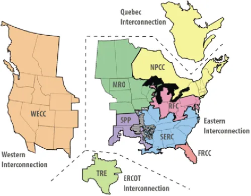
Transmission planning has historically been done on a regional (United States1) or country-wide basis (in Europe); the planning areas in the western United States, for example, are shown in Figure 1-1. In the past, these regions were able to plan inde-pendently as their systems were not tightly interconnected and fossil generation could be sited within the regions to meet electric demands. Unlike fossil generation, however, renewable energy generators are location constrained. That is, renewable energy genera-tors can only economically be sited in areas with strong natural resources. As seen in Figure 1-2 through Figure 1-5, these resources are not distributed evenly across regions or nations and are not correlated with areas of high load (along the coasts in the United States and in northern Europe). Accessing these resources requires significant transmis-sion investment as detailed in reports such as the Eastern Wind Integration and Transmission Study [42], and dramatically displayed in 2011 when a $12 billion wind farm proposed in the Texas Panhandle was cancelled due to lack of transmission capacity [26].

1_{“To call the U.S. grid balkanized would insult the Macedonian.” Mark Spitzer, former FERC Chairman.}

(19)

19

Figure 1-1 Western Planning Areas [70]

Figure 1-2 Wind Resource Map of Europe [23]

Figure 1-3 Solar Resource Map of Europe [24]

(20)

20

The historic conditions which allowed electric areas to be planned separately no longer hold true. Location-constrained renewables are being considered to replace location-unconstrained fossil generation. The once independent systems are becoming more interconnected and operational issues (termed seams issues) resulting from planning and operating interconnected systems independently are growing. To cope with these and other issues, larger areas are being considered for transmission planning. In Europe, the European Network of Transmission System Operators (electricity) has been tasked with developing European-wide transmission plans. In the United States, the Department of Energy has sponsored transmission planning across the three electrical interconnects, shown in Figure 1-6 [19], [20], [68], and the Federal Electricity Regulatory Commission has mandated wider regional planning [25].

Figure 1-4 Wind Resource Map of the United States [44]

Figure 1-5 Solar Resource Map of the United States [45]

(21)

21

Figure 1-6 Three Electrical Interconnections in the United States

Under the most favorable conditions, planning the transmission network is a non-trivial problem. The transmission network is an infrastructure system with investments characterized by their high capital costs and long lifetimes. Each transmission line is a lumpy investment with costs ranging from $1.1 million to $4 million per mile depending on the voltage rating of the line [3]. These cost estimates, however, are more realistically viewed as lower bounds. For example, aesthetic and environmental concerns elevated the cost of a 69 mile line in Connecticut to $1.3 billion compared to the $76 million predicted using the costs above [47]. Transmission investments must also be planned prospectively. The time from a transmission line’s selection for construction to energization is five to ten years. In that time, the need for the investment may be eliminated, for example a new power plant may have been constructed elsewhere in the system, or exacerbated, for example a boom in the economy prompting higher electricity demands. Once

(22)

construct-22

ed, transmission lines have operating lifespans of 40 to 50 years2. As part of a networked system, the effects of adding capacity are often non-intuitive. In some cases, adding capacity to the system can actually exacerbate rather than relieve problems.

Planning the transmission network to incorporate high renewable generation penetra-tions is complicated both by the geographic scope required and the uncertainty in the development of future generation. The growth of the location constrained generation is dominantly policy driven. These policies, however, are unstable due to changes in political will. For example, in the Unites States the development of wind resources has been tightly coupled and fluctuated with the Production Tax Credit (PTC) which subsi-dizes wind power production. This policy uncertainty is compounded by the mismatch in generator build time and transmission build time [52]. Location-constrained generators such as wind and photovoltaics require a two to five year construction timeline, while transmission lines require five to ten years to plan and construct. With generator build times significantly lower than those for transmission, planners are forced to either antici-pate new generation and build potentially unnecessary infrastructure or be reactive in building new transmission, potentially discouraging new generation investment.

Tools to support this new type of wide-area stochastic planning do not yet exist. There are models which demonstrate that new capacity is needed, for example the ReEDS model [60]; however, these models lack the technical detail required to examine specific plans. An example of the plans produced by the ReEDS model, shown in Figure 1-7, identifies capacities between grossly aggregated regions, but does not have the detail required to specify investments (eg a 500kV double circuit line between two specific system buses). There are also indicative transmission plans, the most well-known of these developed by American Electric Power (AEP) and shown in Figure 1-8. These indicative plans, also sometimes referred to as crayon plans, have not been economically or techni-cally evaluated; these crayon plans are also not created using underlying models or other scientific rational. Plans such as the AEP proposal are also often viewed with skepticism

2_{In reality, transmission lines are rarely if ever decommissioned. The wires, pylons and insulators are}

(23)

23

by regulators and other stakeholders when they are proposed by the transmission compa-nies which would profit from their construction.

(24)

24

Figure 1-7 ReEds Transmission Expansion Planning Results from the Renewable Electricity Futures Study

(25)

25

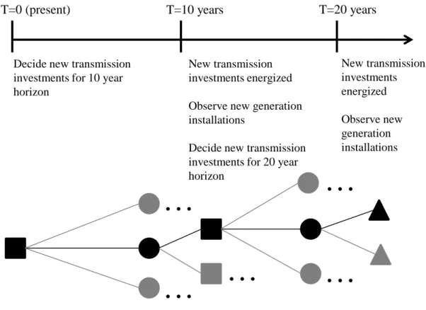
Tools to guide transmission planners toward high-value investment options must capture the temporal and technical details inherent to the problem. While the technical models are well defined, the temporal characteristics are less well framed. Given the stochastic and temporal characteristics, the planning problem can very naturally be represented as a decision tree as shown in Figure 1-9. Following a single path (darkened) through the decision tree, the present day decision (T=0) is what new transmission lines should be added. These lines are planned without knowing where the new generation will be added to the system. While these new transmission lines are being sited and construct-ed, new generation is being added to the system. In the two-stage model presented in Figure 1-9, both the new generation and new transmission lines come online in year ten. In year 10, the system planner can observe the new generation investments and with this new knowledge plan new lines to come online in year 20. When the full problem is enumerated and solved in this framework, discussed further in 1.2.3, the value of any transmission investments today is dependent on how well it performs across a variety of future scenarios.

(26)

26

Figure 1-9 Decision Tree Representation of the Multi-Stage Stochastic Transmission Expansion Problem with Uncertainty in Future Generation

In a standard decision tree representation, squares represent decisions points and circles represent the realization of an uncertain parameter or variable. In this case, the squares represent the selection of new transmission lines (each spoke coming from the square represents a distinct investment option) and the circles represent the resolution of both the quantity and location of new generation (each spoke coming from the circle repre-sents a specific future scenario of generation expansion).

T=0 (present) T=10 years T=20 years

Decide new transmission investments for 10 year horizon

New transmission investments energized Observe new generation installations

Decide new transmission investments for 20 year horizon New transmission investments energized Observe new generation installations

. . .

(27)

27

1.1 Transmission Expansion Planning

Transmission planning is often used colloquially as an omnibus description for the entire process of adding a new transmission investment to the existing system. This process involves deciding on the new assets to be added, reliability analyses, cost-allocation and siting and routing for new lines. Traditionally, cost allocation and siting have been the most contentious issues in transmission expansion planning. Cost allocation is the deter-mination of who pays for the new multi-million dollar investment and siting is both the determination of the geographic route and permitting of that route. Siting is a contentious issue because transmission towers and lines belong to the class of locally unwanted land uses (LULUs) which reduce property value. It is also one of the few pathways that local authorities and stakeholders have to block lines for environmental, aesthetic or economic reasons. As shown in Figure 1-10, these processes are not independent but instead inform one another. For example, the expansion plan decided upon may fail the required reliabil-ity analysis or stakeholder input may require a transmission line to be rerouted. With the new rerouting, the transmission line may no longer be an economic solution. For the purposes of this dissertation, however, transmission expansion planning will be more narrowly defined to refer to the selection of new transmission assets.

(28)

28

Figure 1-10 Steps in the Transmission Planning Process 1.1.1 Motivations for Transmission Expansion Planning

Transmission investments are made for two major reasons: improving the reliability of the power system and lowering the cost to operate the power system. These investments can be transmission lines (overhead lines or underground cables) or additional support equipment such as protection systems, transformers or reactive power controls which can improve the operation of existing transmission lines. The traditional treatment of trans-mission expansion planning frames the problem as trading-off between economic benefits through lower system operating costs and the investment costs of new transmission investments. In this view, the reliability of the system is treated as a constraint in the planning process. There are, however, streams of research which consider reliability probabilistically and explicitly within a risk context [14].

The reliability requirements of the power system can be represented both with eco-nomic costs and engineering constraints. From an ecoeco-nomic perspective, the power system should be able to meet the electric demand all hours of the year with very low probability of non-served demand, more generally called electricity non-served (EENS) or power non-served (PNS)3. The engineering constraints on the system are more

3_{In the United States, the a common loss of load expectation used is one day in ten years.}

Select Transmission Lines Operational Reliability Analysis

Cost Allocation Siting/Routing

Stakeholder Feedback

(29)

29

cated. The majority of power flows through the transmission network are alternating current (AC) as shown in Figure 1-11. With alternating current, the power flowing through each line on the transmission network fluctuates with time at a set frequency (60 hertz in the US and 50 hertz in Europe) and a set voltage level (for example 345kV). If the frequency and voltage are not maintained within tight bounds, some demand may not be met (brownouts) and/or the power system may totally collapse (blackouts). These bounds must be maintained even if there are large disturbances on the power system, such as a generator unexpectedly failing or a storm disabling a transmission line. These failures of individual pieces of equipment are called contingencies, and the most common contingency scenarios to consider contain the failure of any one single component, referred to in the field as n-1 contingency analysis. Investments in the transmission network can alleviate these threats by, for example, providing alternative routes for power to flow or providing voltage or frequency support directly.

Figure 1-11 Illustration of Alternating Current Power

Investments in the transmission network can lower the operating costs of the power system by facilitating access to lower cost generation sources. There are areas of the power system which experience congestion. Like traffic congestion, congestion in the power system means that the flow into or out of a specific area is limited. For example, a hydro power plant may have a capacity of 1,000 MW but may be connected to the system with a transmission line capable of carrying only 500 MW to the demand center. As a result of the congestion at the hydro power plant, a more expensive generator closer to

Time

(30)

30

the load must be dispatched. If a new transmission line is added to the system which connects the hydro power plant to the demand center with an additional 500 MW, the congestion in the system will be reduced. The more expensive plant will no longer be dispatched, and the cost of operating the system will be lessened.

New transmission investments can also reduce the losses in the system. Losses in the power system reflect electricity that is produced by generators but does make it to the demand in order to do useful work. Instead, this useful energy is lost to the system, for example through production of heat in transmission lines. In the United States, for example, approximately 7% of all generation, or 262,000 MWh is consumed annually by losses across the transmission and distribution networks [21]. Using a back of the enve-lope calculation, this implies that in the United States $15.7 billion is spent annually on non-productive generation4. Losses in transmission lines can be reduced either by in-vestment in new equipment to increase the operating voltage transmission of lines or by adding new transmission lines such that less power flows on each line.

The addition of transmission capacity can also lower costs by easing operational and market restrictions within the power system. For example, when bordering areas are well connected, the generation reserves burden can be shared at a lower cost rather than borne individually [36]. Transmission capacity can also help reduce the effects of variability inherent to wind and solar generators by providing access to flexible generators and capitalizing on the reduction of variability as the geographic scope considered increases [31]. By eliminating congestion in the network, transmission capacity investments can also help mitigate market power in electricity markets [65].

More recently, it has also been explicitly recognized that transmission may be con-structed for a third reason, the meeting of public policy goals. These public policy lines may not be justified under either the economic or reliability criteria above (for example, see Section X in FERC Order 1000 [25]). The dominant public policy goal considered in today’s transmission expansion planning studies is the inclusion of renewable resources.

(31)

31

Because these resources are location-constrained, they cannot be effectively accessed without new transmission investments.

1.1.2 Timescales for Transmission Expansion Planning

Transmission expansion planning takes place on multiple timescales ranging from 5 to 30 years. These timescales, roughly outlined in Table 1-1, have different foci and require varying degrees of technical accuracy.

Table 1-1 Timescales for Transmission Expansion Planning (Very) Near Term Mid-Term (Tactical) Long-Term (Strategic)

Very Long Term Horizon 0-5 years 5-10 years 15-20 years 25-30 years

Major Focus Reliability

Reliability and Econom-ics Economics and Scenario Analysis Scenario Analysis Load Flow Type AC Load Flow DC Load

Flow DC Load Flow

Transportation Load Flow Representative Models Dynamic Simulation AC Optimal Power Flow Optimal Transmission Expansion Planning DC Optimal Power Flow Optimal Transmission Expansion Planning DC Optimal Power Flow Optimal Trans-mission Expansion Planning Pipes and Bubbles

The shortest time scale considers investments to be made in the next five years. Eco-nomic issues may be considered, but the major focus of this timescale is reliability. In order to capture near-term reliability issues, the types of models used have very high technical fidelity. The investments considered on this timescale are more likely to be transformer upgrades, reconductoring, or other projects related to existing transmission lines rather than new transmission lines in new rights of way. Realistically, this is be-cause it is unlikely that a new line could be permitted and constructed within a five year period.

Mid-term or tactical planning includes both reliability and economic foci. Looking five to ten years out, the investments identified in this horizon may present longer-term

(32)

32

fixes to the problems identified in the near-term planning or address structural rather than temporary economic and reliability issues. These investments may be identified using expert judgment or an optimal Transmission Network Expansion Planning model (TNEP). Different types of optimal TNEP models will be explored in 1.2, but briefly, the goal of such models is to algorithmically minimize the total system cost trading off generation, non-served energy and transmission investment costs. The models used to identify and evaluate transmission solutions in mid-term planning are of lower technical fidelity than those in the near-term horizon. These models typically use an approximation of the AC load flow called the DC load flow. The DC load flow simplifies the AC load flow by assuming the magnitude of the voltage sine waves (shown in Figure 1-11) at each node remains constant. The most common form of the DC load flow is also linearized, allowing it to be integrated into traditional linear or mixed-integer linear optimization models. Mid-term planning is designed to identify new transmission lines (either green-field development or re-enforcing an existing transmission line) that would then iterate with the more technical reliability analyses, siting, and cost allocation procedures identi-fied in Figure 1-10.

Long-term or strategic planning is used to guide mid-term planning toward higher-value transmission solutions and for scenario analysis. The most common use is scenario analysis; for example, most high renewable penetration studies are strategic planning studies. Like mid-term planning, the models used in strategic-planning studies are based on DC load flows and both expert analysis and optimal transmission expansion algo-rithms are used. The models used for long-term studies are also most likely to be abstractions of the real system with aggregated generation and demand buses. Unlike mid-term planning, the transmission lines identified in a long-term planning study are unlikely to be formally considered as potential investments.

Finally, the furthest time horizon typically considered for transmission planning is 25-30 years. On this timescale, the power system is very abstracted. If power flows are modeled in a system, they are often assumed to be directable, simplifying the physics driven flows but continuing to respect capacity restraints of the lines. More often,

(33)

sys-33

tems are aggregated to a pipes and bubbles model. In this approach, large areas are aggregated to a single load/generator, or bubble, and the transmission lines between areas aggregated into a single transfer capacity, or pipe. For example, a pipes and bubble approach might consider each country in Europe as a single bubble and connect a single pipe to each adjacent country. This type of modeling examines how much transfer capacity might be useful between regions, but does not have the technical detail to identify specific transmission investments.

The work presented in this dissertation focuses on the mid-term and long-term plan-ning horizons. The emphasis is on using information from the long-term planplan-ning horizon to inform mid-term planning investments. With this, the planning emphasis is also on the major economics tradeoff rather than operational reliability.

1.2 Optimal Transmission Network Expansion Planning Model

Formulations

Optimal TNEP models algorithmically balances the investment costs of new lines against reductions in generation and non-served energy costs. Models for the optimal TNEP problem are used to guide system planners toward promising investment choices which are then subject to further operational reliability analysis. The balance of costs is achieved by minimizing annualized systems costs, the sum of annualized investment, non-served energy and generation costs. From an optimization perspective, single-horizon transmission planning falls into one of the hardest problem classes. Transmission network expansion planning is a network problem with non-directable flows and integer investments. It is a combinatorial optimization problem and classified as an NP-Complete problem for which no solution method exists in polynomial time. The number of potential plans for a single investment horizon grows exponentially with respect to the number of potential investments (2n where n is the number of investment options). A very small problem with only 10 possible transmission investments has 1,024 different plans possi-ble, while a problem with 100 possible transmission investments has over 1030 plans possible. A more realistically sized problem with 1,000 possible investments has over 10300 possible plans.

(34)

34

The full transmission expansion planning problem is a mixed-integer non-linear problem (MINLP). The integer constraints arise from the transmission investment variables which represent the lumpy investments. The non-linearity arises from represent-ing the physics-driven flows of electricity within the system. The complete DC load flow formulation of the MINLP formulation is given equations Eq. 1 through Eq. 8. The objective function, given in Eq. 1, reflects the tradeoffs typical to mid-term and long-term planning horizons. In Eq. 1, the total cost of the system including new transmission costs, generation costs and non-served energy is minimized. Kirchoff’s first law, that demand at each bus must be equal to the sum of flow in to the bus, plus generation at the bus, and served energy at the bus minus flow out of the bus is given in Eq. 2. The non-linearities of the optimal transmission expansion problem are shown in Eq. 3 and Eq. 4 which represent flows on the networks. The first non-linearity results from the fact that flows on transmission lines are inversely proportional to physical properties of the line, captured in the reactance of the line and directly proportional to the sine of the differ-ence in voltage angles between buses. The second non-linearity is given in Eq. 4, which describes flow equation for new lines and the non-linearity results from the multiplication of the integer investment variable by the flow.

Eq. 1 ∑ (∑( ) ∑ ) s.t. Eq. 2 ∑ ∑ i=1,…,I Eq. 3 ⁄ ( ) k K0 Eq. 4 ⁄ ( ) k K+ Eq. 5 k K+ Eq. 6 i=1,…,I

(35)

35

Eq. 7 n=1,…,N

Eq. 8 k=1,…,K0

Indices and Sets:

i index of buses

k index of circuits

i(k), j(k) index of terminal buses of circuit k

h index of load hours

n index of generators

K+ set of candidate circuits

K0 set of existing circuits

Ωi set of all circuits connected to bus i

σi set of all generators located at bus i

H number of load hours

I number of buses

M number of candidate circuits

N number of generators

Parameters/Constants

cg generator costs [$/MW]

ct annualized cost of candidate circuits [$]

cμ cost of non-served energy [$/MW]

d bus demands [MW]

fmax circuit capacities [MW]

gmax generator capacities [MW]

X circuit reactances [pu]

b per unit base

(36)

36

θi,h bus voltage angle

Positive Variables

fk,h circuit flow [MW]

θk,h positive bus voltage angle component across circuit k

gn,h generator output [MW]

μi,h non-served energy [MW]

Binary Variables

xk investment variable

The most common implementation of the TNEP problem is a linearized formulation. The linearized formulation of the problem allows for the use of well characterized traditional optimization routines for linear and mixed integer linear programs (LPs and MILPs). In order to linearize the MINLP, Eq. 3 and Eq. 4 are simplified to Eq. 9 and Eq. 10 by assuming small angular differences in the network. When angular differences are small, the sine of an angle may be approximated the angle itself (in radians). The non-linearity left in Eq. 10 can be linearized for traditional optimization methods through the use of the disjunctive formulation such as in [8]. Other optimization methods, such as meta-heuristics, are blind to the non-linearity in Eq. 10 as they do not rely on linear relaxations of the full problem to establish bounds on the objective function for the algorithm to proceed.

Eq. 9 ⁄ ( ) Eq. 10 ⁄ ( )

For clarity, the formulation presented thus far is the most basic expression of the problem. It does not include losses or the n-1 contingency considerations discussed above or any other reliability constraints. There are, however, linear representations of the

(37)

37

losses that may be integrated into MILP formulations of the optimal transmission expan-sion planning problem (see for example [1] [42] or [59]). Likewise, the n-1 contingency constraint has been included in transmission expansion planning models, but it is general-ly considered in an iterative fashion where the optimal transmission expansion planning model determines a test plan, n-1 reliability is examined, and new constraints are passed back to the optimal transmission expansion planning model (see for example [50] or [53]).

The most common optimal TNEP formulations are both deterministic and static. De-terministic models do not consider the many uncertainties that face power system planners, including uncertainty across fuel prices, policies affecting the power system and new generation locations. As deterministic models simplify the uncertainty facing planners, static models simplify the time horizons planners consider. Although new transmission lines have life spans of more than 40 years, static models consider only a single future year. This static-deterministic model formulation is the one presented above in Eq. 1 through Eq. 8.

Due to the computational complexity of the problem, the static-deterministic formu-lation is the most studied in the academic literature. Beginning with LL Garver’s foundational planning paper in 1970, researchers have applied a variety of approaches to solve the problem, including linear optimization [26], dynamic programming [18], decomposition techniques [8], engineering heuristic guided searches [32][59] and meta-heuristics [54] [58][71]. The dominant approach for transmission expansion planning in the late 1990s to early 2000s used traditional optimization techniques for MILPs. Follow-ing the thrust on traditional optimization methods in the early 2000s has been an emphasis on meta-heuristic methods. A variety of meta-heuristic models ranging from genetic algorithms [58] to simulated annealing [54] have been applied to the transmission expansion planning, though no one meta-heuristic approach has been found to be most effective.

While the static-deterministic problem is the most studied formulation, the problem considered in this dissertation requires multi-stage stochastic modeling. The effects and

(38)

38

current literature of multi-stage transmission planning modeling are discussed in 1.2.1 and stochastic planning in 1.2.2. Finally, the combination of stochastic and multi-stage modeling are considered in 1.2.3.

1.2.1 Multi-Stage Planning

Transmission lines are capitally intensive investments with economic lifespans of 40 or more years. Over the lifespan of these investments, the power system will continue to evolve. Existing generators will retire, and new generators will be added. Loads will increase and decrease with the economy and new development patterns. Fuel prices will fluctuate as will national policies and environmental regulations. All of these changes will affect the value of a transmission plan. A transmission expansion model, however, cannot capture all of these varying timescales. Instead, modelers simplify the number of time horizons to capture the most important details.

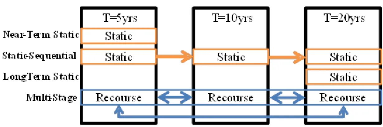
The most common simplification made in TNEP models is to consider only a single investment decision stage. With this simplification, modelers plan for a specific target year. Traditionally, plans have been constructed for mid-term horizons (5-10 years) or long-term horizons (15-20 years). The static case is the one most commonly studied in the literature (see above citations) and is also the most common in industry and policy studies. The most prominent renewable integration/transmission studies are examples of long-term static studies [17][42][43]. A less common approach is to consider a series of static time horizons. As shown in Figure 1-12, the static sequential approach plans for the first time horizon, carries over the new investments from the first stage as constraints to the second stage, plans for the second stage, etc. The WECC TEPPC planning approach using a 10 year planning process and integrating those lines as constraints into the 20 year horizon is an example of the static sequential approach [68].

(39)

39

Figure 1-12 Comparison of Static, Static Sequential and Multi-Stage Modeling

The static horizon simplifications are problematic because either economies of scale are not captured in the modeling or pent up demand for new transmission capacity overstates the desirability of large lines. As an example of the economies of scale in the transmission system, on a thermal-capacity basis, a 345kV double circuit line (tower with two sets of conductors) costs $1,333/MW-mile while a 765kV single circuit line (tower with one set of conductors) costs 70% less, $413/MW-mile5. If a mid-term horizon is used, there is a limited time for demands to grow, and the need for larger lines is never recognized. On the other hand, with a long-term horizon and the assumption of no new transmission over 20-30 years, there is a pent-up demand for new transmission and large lines are almost exclusively selected.

This concept is illustrated in a simple three bus model in Figure 1-13. In this model, a single load exists at Bus A with generators at Buses B and C. There are also two investment options: a 750 MW line from Bus A to Bus B for an annualized cost of 5 million USD (MUSD) or a 1,500 MW line in the same corridor for 7.25 MUSD annually. In the traditional myopic formulation, only the load in year 10 would be considered. In this case, only 400 MW of transmission capacity is required to meet the load and the least cost investment is the smaller 750 MW line. If, however, a second time horizon, 25 years, is considered the demand has grown to 1,500 MW and now an additional 900 MW of capacity is required to meet the demand at Bus A. The lowest-cost option is now the

(40)

40

more expensive but larger line. To include the effects of multi-stage modeling in optimal transmission expansion planning models, the objective function explicitly includes costs on multiple time horizons and inter-temporal investment constraints are added. An example of an objective function considering two time-horizons is given in Eq. 11. In Eq. 11, the costs are discounted by a factor, , and summed across each annual time horizon,

y....Y.

Figure 1-13 Test System for Time Horizon Simplification

Test system assumes cost and capacity characteristics approximating a 345kV double circuit line and 765kv single circuit line at 100 miles length.

Eq. 11 ∑ [ ∑ (∑( ) ∑ ) ]

These effects have also been explored in a case study on the Spanish transmission network. The case study considered a reduced-order system with 701 existing 400kV and 700kV lines. Five five-year periods were considered between 2015 and 2035. First, each

C

10 year demand: 1,000 MW

25 year demand: 1,500 MW

Capacity: 1,500 MW

Capacity: 400 MW

300 MW

A

B

Existing Line Potential New Line

(41)

41

time period was planned statically (individually) with 279 candidate lines considering three different capacities assuming 1% load growth annually. As seen in Figure 1-14, there are five lines constructed in the 2015 plan that are no longer required in the 2035 plan. The planning exercise was then rerun using a more limited set of 16 potential transmission investments and two time horizons (2015 and 2035) to directly compare a multi-stage approach to the static-sequential results. As shown in Figure 1-16, the static and multi-period models produce different first stage decisions in 2015. The static approach selects seven first stage investments (four 400 MW lines, 0 750 MW lines and three 1500 MW lines) while the multi-stage model selects only five lines (one 400 MW line, one 750 MW line and three 1500 MW lines). This case study clearly illustrated that even in a small system, the static sequential approach does not mirror the results pro-duced by the true multi-stage model.

Figure 1-14 Spanish Case Study Static Results for 2015 (L) and 2035 (R) Note that only lines which are not consistent across one or more time horizons are

shown. Additional 1,500 MW line Additional 1,500 MW line Additional 400 MW line Additional 1,500 MW line Additional 1,500 MW line

400 MW

_{750 MW}

_{1500 MW}

(42)

42

Figure 1-15 Spanish 2015 Case Study Dynamic Programming Results (L) and Static Planning (R)

This type of multi-stage modeling is relatively rare in the academic transmission ex-pansion planning literature. Examples of the relevant literature are given [5], [9],[64], and in [35]. Common to these works is an emphasis on investment timing rather than captur-ing effects of economies of scale or rectifycaptur-ing issues with myopic planncaptur-ing. This may in part be due to the small test systems with limited investment options used in the academic studies. For example, [9] considers 23 investments, of which only 13 are transmission lines, across a system with 157 buses. By comparison, there are more than 2,000 buses in the electricity system in the western United States over 200kV. Each of these works is also focused on the demonstration of a new algorithm rather than an analysis of the results. The first three works demonstrate heuristic algorithms while [5] explores a branch-and-bound algorithm with a transportation-based transmission work (respects only Kirchoff’s first law).

One reason that multi-stage models are not as popular in the literature is the compu-tational complexity added by the intertemporal constraints. The addition of multiple time stages again increases the size of the optimization problem. The growth of the number of

-10 -8 -6 -4 -2 0 2 4 35 36 37 38 39 40 41 42 43 44

400 MW

_{750 MW}

_{1500 MW}

(43)

43

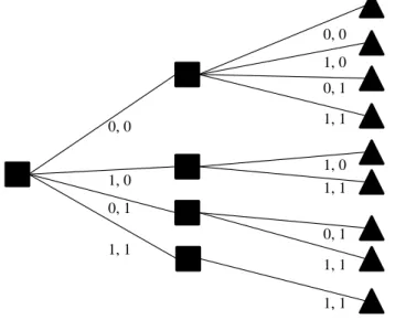
possible plans that must be considered is demonstrated in a two-horizon expansion planning problem with two possible investments. As shown in Figure 1-16, if only the first stage problem is considered, there are four possible transmission expansion plans to evaluate. On the other hand, when two stages are considered, there are now nine possible two-stage transmission plans to consider.

Figure 1-16 Expansion of the Decision Space Including Multiple Time Horizons

While true multi-stage modeling is not common to industry methods, heuristic meth-ods have been used to span time horizons. For example, in the Southwest Power Pool’s Integrated Transmission Planning, three time horizons are considered (near term, 10 years and 20 years) [61].While the three timescales are never formally integrated, in-vestments identified in longer terms studies are highlighted in the near term studies. Likewise, Red Electrica in Spain uses a long term planning models in to inform medium-term transmission planning [16].

1.2.2 Planning Under Uncertainty

Almost all industry and academic transmission expansion planning models consider specific scenarios with perfect knowledge. That is, the modeler assumes that all future demands, fuel prices, generator locations and reliability issues are known. In reality, of

0, 0 1, 0 0, 1 1, 1 0, 0 1, 0 0, 1 1, 1 1, 1 1, 0 1, 1 0, 1 1, 1

(44)

44

course, planners have very imperfect knowledge about the future. Natural disasters destroy infrastructure and cause major changes in fuel prices. Technological break-throughs produce new generation types not even known to today’s planners. In order to capture some of this uncertainty, planning models can try to produce transmission plans with low costs across a variety of different futures.

Including uncertainty in the objective function affects the operational costs. As shown in Eq. 12, the investment decisions made are not based on the individual scenario,

s, but the operational costs all become scenario dependent. Each scenario is also weighted

by its probability, ps. There are both random and non-random sources of uncertainty to be considered in the transmission expansion planning problem. Random uncertainty, such as the outage of a component, the evolution of fuel prices, and demand growth can be modeled probabilistically based on future projections of historic data. Non-random uncertainties such as the location of new generation, regulatory changes, and the devel-opment of new technologies, however, are do not historic datasets on which to draw.

Eq. 12 ∑ [∑ (∑( ) ∑ ) ]

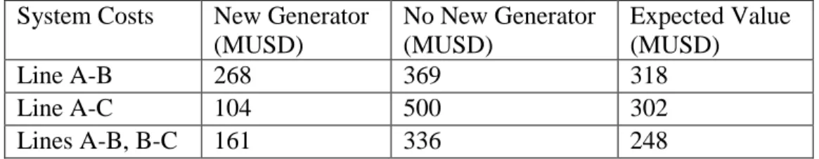
As an illustration of uncertainty’s effects on transmission expansion in a small ex-ample, take the three bus example now shown in Figure 1-17. In this iteration of the model, a new low-cost power plant may be constructed at Bus C and three different investment options are presented by the planner. The total system costs assuming each transmission and generation scenario are given in Table 1-2. If the planner had perfect foresight and knew that the plant would not be built, the lowest cost investment option would be to build Lines A-B and B-C. Note that because the system is networked, the most intuitive solution, building Line A-B only, is not the lowest cost option in any scenario. Instead, building the additional line between Buses B and C allows the lower cost plant to meet the entire load at a lower cost by sending power across both the new lines and the existing line between Bus A and Bus C. On the other hand, if the planner had perfect foresight and knew the new generator would be built, the lowest cost option is to build only the additional capacity between Bus A and Bus C. If the planner assumes

(45)

45

the generation is built and only adds only Line A-B, but the generation developer pulls out, the system becomes very expensive, nearly a factor of five more, to operate.

Cost (MUSD) Capacity (MW) Line A-B 5.0 750 Line A-C 5.0 750 Line B-C 3.0 500

Figure 1-17 Test System for Uncertainty Simplification

Table 1-2 Scenario Costs for Uncertainty Test System

System Costs New Generator (MUSD) No New Generator (MUSD) Expected Value (MUSD) Line A-B 268 369 318 Line A-C 104 500 302 Lines A-B, B-C 161 336 248

The most common place to find uncertainty considered in for transmission expansion planning is in the area of planning for reliability. As a field, probabilistic transmission expansion planning focuses on random uncertainties, specifically failure of components [14],[34]. With this approach, the uncertainty is treated as a constraint (eg the system must survive with at least a set probability) [14]. This framing with uncertainty as a

C

Demand: 1,250 MW

A

B

?

Capacity: 1,500 MW

Capacity: 400 MW

Cost: $30 MWh

Cost: $50 MWh

Capacity: 300 MW

Cost: $5 MWh

300 MW

(46)

46

constraint is not appropriate considering uncertainties affecting operational costs. The reliability tests are binary, either the system fails or survives. With operational costs, there is not a failure metric but rather a distribution of operational costs. Plans can be differentiated by the expected value of these costs or other decision metrics of interest such as minimum regret.

Planning across uncertainties again increases the size of the planning problem. As a result, the approach used by most of the academic planning literature does not truly optimize across uncertainties. Instead, the general strategy is to generate a variety of plans by optimizing deterministic scenarios. The plan is then evaluated under different scenarios, and the plan with the best decision metric is selected. For example, Sozer generated scenarios using Monte Carlo sampling and then selected an optimal plan according a multiple comparisons to the base (MCB) metric [62]. Zhao also optimized individual scenarios to create transmission expansion plans and then tested the reliability of each transmission plan under the other scenarios [72]. Likewise, Bustamente-Cedeno and Arora used scenarios to generate potential transmission expansion plans [11]. The optimal transmission expansion plans was then selected from amongst the set using expected value and minimum regret decision metrics. These approaches reduce the computation burden of solving the stochastic problem, but likely miss the plan which performs best across uncertainty as demonstrated by [41].

Each hour of the year modeled in TNEP may also be framed as an uncertainty. For computational reasons, the full 8,760 hours each year are rarely modeled in an optimiza-tion problem. Instead, a selected number of hours (for example those representative of peak, intermediate and baseload demand) are modeled. The duration of each representa-tive hour may be reconsidered as the probability for that load profile and the goal of the optimization is to produce the highest expected value. This is the framing used in [31] though not explicitly modeled in a stochastic framework.

1.2.3 Stochastic Multi-Stage Planning with Recourse

Combining multi-stage modeling and stochastic modeling explicitly models the full optimization problem of transmission expansion planning under uncertainty. The problem

(47)

47

now explores four major sets of tradeoffs summarized in Table 1-3. First, the optimiza-tion considers the balance of current and future costs. Second, the optimizaoptimiza-tion considers the tradeoff between economies of scale and current costs. Larger lines capitalize on economies of scale, but they are also more expensive to build in the near term. By combing stochasticity and multi-stage modeling, the tradeoff between economies of scale and adaptability is also included. If large lines are constructed to capitalize on economies of scale but those interconnected areas experience less than predicted generation expan-sion, the investments may be underutilized. On the other hand, building and under-estimating generation may result in congestion, underutilization of the new generation and higher operational costs. Finally, the optimization respects the fundamental tradeoff between investment and operational costs.

Table 1-3 Summary of Tradeoffs Considered in Stochastic Multi-Stage Models Tradeoffs

Current Costs vs Future Costs Current Costs vs Economies of Scale Economies of Scale vs Adaptability

Investment Cost vs Operational Costs

By combining multi-stage and stochastic modeling, the structure of the objective function changes. An example of an objective function for a single investment with two decision-stages and two uncertainty-stages model is given in Eq. 13 and a graphic illus-tration of the problem in Figure 1-18. In Eq. 13, the cost to minimize is the cost of first stage transmission investments, the expected first-stage operational costs, OC1, and the discounted sum of second stage investment costs and second-stage expected operational costs, OC2. As shown in Figure 1-18, for a single investment the tree grows to 12 unique combinations of first stage investments, second stage investments, first stage uncertainty and second stage outcomes.

(48)

48

Eq. 13 [ ] [ ]

Figure 1-18 Single Investment, Two Decision-Stage, Two-Uncertainty Stage Prob-lem Illustration

After each decision, x, the current system state is shown in brackets. NB, once the single line has been selected for investment, no further transmission investment options exist.

Important to note in Eq. 13 is that the second stage decision is contingent both upon the first stage decision and the outcome of the first stage uncertainty. This ability to reconsider investment decisions after the uncertainty has been revealed is referred to as recourse. Access to recourse is what differentiates this stochastic multi-stage modeling from the deterministic multi-stage modeling where a single trajectory for all time is selected. In this modeling context, the most important outcomes are the stage one decision investments. After these investments are made, the uncertainty is revealed, and the process is rerun given the new starting state of the world. Again, although only the

[0] [1] [0, s1] [1, s1 s1 s2 s2 s1 [0, s2] [1, s2] [1, s1] [1, s2] s3 s4 [0, 0, s1, s3] [0, 0, s1, s4] [0, 1, s1, s3] [0, 1, s1, s4] [0, 0, s2, s3] [0, 0, s2, s4] [0, 1, s2, s3] [0, 1, s2, s4] [1, 1, s1, s3] [1, 1, s1, s4] [1, 1, s2, s3] [1, 1, s2, s4] s3 s4 s3 s4 [x₁, x₂, s₁, s₂]