Computational Approaches to Modeling the Conserved
Structural Core Among Distantly Homologous Proteins
by
Matthew Ewald Menke
Submitted to the Department of Electrical Engineering and Computer
Science
in partial fulfillment of the requirements for the degree of
Doctor of Philosophy in Computer Science
at the
MASSACHUSETTS INSTITUTE OF TECHNOLOGY
September 2009
©
Massachusetts Institute of Technology 2009. All rights reserved.
ARCHIVES
Author
Department of Electrical Engineering and Computer Science
August 19, 2009
Certified by
Bonnie Berger
Professor of Applied Mathematics
Thesis Supervisor
/7 /-,
Accepted by...
Professor Terry P. Orlando
Chair, Department Committee on Graduate Students
MASSACHUSETTS INSTr'IJTE
OF TECHNOLOGY
SEP
3 0 2009
Computational Approaches to Modeling the Conserved Structural
Core Among Distantly Homologous Proteins
by
Matthew Ewald Menke
Submitted to the Department of Electrical Engineering and Computer Science on May 29, 2009, in partial fulfillment of the
requirements for the degree of
Doctor of Philosophy in Computer Science and Engineering
Abstract
Modem techniques in biology have produced sequence data for huge quantities of proteins, and 3-D structural information for a much smaller number of proteins. We introduce several algorithms that make use of the limited available structural information to classify and an-notate proteins with structures that are unknown, but similar to solved structures. The first algorithm is actually a tool for better understanding solved structures themselves. Namely, we introduce the multiple alignment algorithm Matt (Multiple Alignment with Transla-tions and Twists), an aligned fragment pair chaining algorithm that, in intermediate steps, allows local flexibility between fragments. Matt temporarily allows small translations and rotations to bring sets of fragments into closer alignment than physically possible under rigid body transformation. The second algorithm, BetaWrapPro, is designed to recognize sequences of unknown structure that belong to specific all-beta fold classes. BetaWrap-Pro employs a "wrapping" algorithm that uses long-distance pairwise residue preferences to recognize sequences belonging to the beta-helix and the beta-trefoil classes. It uses hand-curated beta-strand templates based on solved structures. Finally, SMURF (Struc-tural Motifs Using Random Fields) combines ideas from both these algorithms into a gen-eral method to recognize beta-structural motifs using both sequence information and long-distance pairwise correlations involved in beta-sheet formation. For any beta-structural fold, SMURF uses Matt to automatically construct a template from an alignment of solved
3-D structures. From this template, SMURF constructs a Markov random field that
com-bines a profile hidden Markov model together with pairwise residue preferences of the type introduced by BetaWrapPro. The efficacy of SMURF is demonstrated on three beta-propeller fold classes.
Thesis Supervisor: Bonnie Berger Title: Professor of Applied Mathematics
Acknowledgments
I am grateful to Lenore Cowen for her help in designing, and, particularly, in evaluating and writing up the algorithms discussed in this paper.
Many thanks to my advisor, Bonnie Berger, for all her technical guidance and finding me funding for all these years. Thanks also to Akamai, Merck, and the National Institute of Health for providing the aforementioned funding.
I would also like to thank my parents for their financial and moral support and, more importantly, for not repeatedly asking me when I was finally going to graduate.
I also want to thank Phil Bradley, Andrew McDonnell, Nathan Palmer, and Jonathan King for their contributions to the development of the BetaWrap and BetaWrapPro algo-rithms.
Roland L. Dunbrack, Jr. generously assisted with with SCWRL.
Much of the work in Chapter 2 of this thesis appeared as "Matt: Local Flexibility Aids Protein Multiple Structure Alignment" in PLoS Computational Biology in 2008. Most of Chapter 3 was published as "Prediction and comparative modeling of sequences directing beta-sheet proteins by profile wrapping" in Proteins: Structure, Function, and
Bioinfor-matics in 2006, volume 63. Chapter 4 has yet to be published. I thank my coauthors for
their permission to include our joint work in this thesis. I would also like to the members of my thesis committee.
Contents
1 Introduction
1.1 Protein Structural Alignment . ...
1.2 Protein Superfamily Recognition from Sequence . .
1.2.1 Protein Profile Hidden Markov Models . . .
1.2.2 Threading ... 1.3 Our Contribution ... 1.3.1 M att . . . . 1.3.2 BetaW rapPro ... 1.3.3 SM URF ... 1.3.4 Conclusions ...
2 Matt: Local Flexibility Aids Protein Multiple Structure
2.1 Introduction ... 2.1.1 Performance Metrics . ... 2.1.2 Our Contribution . ... 2.1.3 Related Work ... 2.1.4 Matt Implementation ... 2.2 Algorithm Overview ... 2.3 Results. . ... ...
2.3.1 The Benchmark Datasets . ...
2.3.2 The Programs to Which Matt Is Compared
2.3.3 Performance ... 2.3.4 p-Value Calculation . ...
Alignment
. . . o..
2.4 Methods... 2.4.1 Pairwise alignment . 2.4.2 Multiple Alignment. 2.5 Discussion. ... 3 BetaWrapPro 3.1 Introduction . . . . 3.2 The Algorithm . . . . 3.3 Results. ... ....
3.3.1 Recognition and Alignment of Sequences
3.3.2 Comparison to Other Methods ...
3.3.3 Recognition of Unknown Sequences . . .
with Known
. . . ° . .
. . . ° .. .
3.4 Materials and Methods . . . .
3.4.1 Sequence Databases . . . .
3.4.2 Pairwise Residue Databases
3.4.3 Structure Databases ... 3.4.4 Training and Testing . . . .
3.4.5 Running Time . . . .
3.5 Discussion ...
3.5.1 Biological Implications . . . 3.5.2 Web Server ...
4 An Integrated Markov Random Field Method for Recognizing Beta-Structural Motifs 4.1 Introduction . . . . 4.2 A lgorithm . . . . 4.3 R esults . . . . 4.4 M ethods . . . . 4.5 D iscussion . . . . 8 44 44 48 51 Structures . . . .° . °. ° ~-l-X---- ---'*-'~-*-1XY- '"--*--L-'"~ _-~-jili~i.^*:-in~i.I-r;- ~--r~.^rs~---^ --- -r~----~--^rr~-^--r~-w~;i,_i~,,,i--~ -;I; =i;n4~-%.^;;xI~nllr ~1;1~,~
-5 Conclusions 87
5.1 Discussion and Future Work ... 87
List of Figures
1-1 HMMER hidden Markov model ... 19
2-1 Overview of the Matt algorithm ... 30
2-2 Matt SABmark performance tradeoff ... .. 37
2-3 Matt Homstrad performance tradeoff ... .. 38
2-4 Comparative beta-propeller alignment . ... . . . 40
2-5 Comparative beta-helix alignment ... . . . 41
2-6 Distinguishing alignable structures from decoys . ... 42
2-7 Assembling sequential block pairs ... ... 45
3-1 The beta-helix and beta-trefoil folds ... .. 54
3-2 Side-chain packing example ... 62
4-1 A 7-bladed beta-propeller ... ... 75
4-2 HMMER hidden Markov model ... 76
4-3 Anti-parallel beta-strand dependencies . ... .. 77
List of Tables
2.1 Homstrad performance comparison . . . . 2.2 SABmark superfamily performance comparison . . . . 2.3 SABmark twilight zone performance comparison . . . . 2.4 Sample multiple structure alignments from SABmark benchmark . 2.5 Discrimination performance on the SABmark superfamily set . . . 2.6 Discrimination performance on the SABmark twilight zone set . . 3.1 3.2 3.3 3.4 3.5 . . . . 36 . . . . 38 . . . . 38 . . . . 41 . . . . 43 Beta-helix cross-validation . . . . Beta-trefoil cross-validation . . . . Beta-helix alignment accuracy comparison . Beta-trefoil alignment accuracy comparison New beta-helices ...
4.1 Our results versus HMMer 3.0 . . . . 4.2 Selected SMURF predictions . . . . A. 1 Solvent inaccessible beta residue conditional probabilities . . . . A.2 Solvent accessible beta residue conditional probabilities . . . . A.3 Solvent inaccessible twisted beta-strand residue conditional probabilities . A.4 Solvent accessible twisted beta-strand residue conditional probabilities . . A.5 Solvent inaccessible twisted beta-strand one-off residue conditional proba-bilities . . . . . . . 61 . . . 61 . . . 64 . . . 64 ... 67
Chapter 1
Introduction
A single protein chain consists of an ordered set of the twenty different amino acids,
typ-ically from 50 to 1000 residues in length. Proteins are termed homologous if they share a common evolutionary origin; since evolution was not observed over time, homology is generally inferred by similarity. Homology can be inferred by sequence similarity when proteins are evolutionarily close, but as their evolutionary relationship becomes more dis-tance, direct inference of protein homology from sequence can become difficult. However, when 3-D structural information is also available, it can be easier to classify proteins. Pro-teins whose folded 3-D structure is known are termed solved protein structures.
The solved protein structures have been grouped together in hierarchical classification schemes such as the Structural Classification of Proteins (SCOP) [73] and CATH (Class, Architecture, Topology, Homologous superfamily) [76]. At the top level of the SCOP hierarchy, proteins are subdivided based on their predominant type of secondary structure: predominantly alpha, predominantly beta, or a combination of the two. Within these broad groups, there is a further subdivision into the fold, superfamily, and family levels of the SCOP hierarchy. Each successive level contains proteins that share progressively greater structural similarity.
In SCOP, at the 'family' level, this translates into a sufficient level of sequence similar-ity to clearly indicate an evolutionary relationship. The level of pairwise sequence identsimilar-ity at the family level is generally 30% or greater. At the 'superfamily' level, sequence identity is significantly lower, but structural and functional similarities indicate a probable common
ancestor. Proteins in the same 'fold' have the same basic arrangement of secondary struc-ture, but may have significant differences in intervening regions. Such proteins may not have an evolutionary relationship.
This thesis is largely concerned with the goals of recognizing, and aligning proteins that belong to the same SCOP superfamily or fold class. We consider two main subproblems: 1) aligning proteins in the same superfamily whose three-dimensional structures are known, so that the similar parts are matched, and 2) predicting when a protein whose sequence is known but whose structure is not should be placed in the same superfamily as a set of proteins whose 3-D structure is known. In some cases, we not only recognize that the protein folds into the appropriate family, but we also predict the sequence-structure alignment.
1.1 Protein Structural Alignment
The problem of constructing accurate protein multiple structure alignments has been stud-ied in computational biology almost as long as the better-known multiple sequence align-ment problem [71]. The main goal for both problems is to provide an alignalign-ment of residue-residue correspondences in order to identify homologous residue-residues. When applied to closely related proteins, sequence-based and structure-based alignments typically give consistent answers even though most sequence alignment methods are measuring statistical models of amino acid substitution rates, whereas most structure-based methods are seeking to su-perimpose alpha-carbon atoms from corresponding backbone 3-D coordinates while mini-mizing geometric distance. However, as has been known for some time [15], these answers can diverge when aligning distantly related proteins; most relevant, it is still possible to find good structural alignments when sequence similarity has evolutionarily diverged into "the twilight zone" [83]. In the twilight zone, distantly related proteins can still share a common
core structure containing regions, including conserved secondary-structure elements and
binding sites, in which the chains retain the folding topology (see [25] for a recent survey). Structural information can align the residues in this common core, even after the sequences have diverged too far for successful sequence-based alignment, because structural similar-
~~~~-ity is typically more evolutionarily conserved [1, 28, 106]. (While divergent sequence with conserved structure is the typical case and the one that structural alignment algorithms that respect backbone order such as Matt seek to handle, there are also well-known examples where structure has diverged more rapidly than sequence; see, for example, Kinch and Grishin [55] and Grishin [37].)
Applications of multiple structure alignment programs include understanding evolu-tionary conservation and divergence, functional prediction through the identification of structurally conserved active sites in homologous proteins [42], construction of bench-mark datasets on which to test multiple sequence alignment programs [28], and automatic construction of profiles and threading templates for protein structure prediction [25, 78]. It has also recently been suggested that multiple structure alignment algorithms may soon become an important component in the best multiple sequence alignment programs. As more protein structures are solved, there is an ever-increasing chance that a given set of sequences to be aligned will contain a subset with structural information available. To date, however, only a handful of multiple sequence alignment programs are set up to take advantage of any available structural data [28, 77].
Pairwise structure alignment programs fall into three broad classes: the first class, to which Matt belongs, are aligned fragment pair (AFP) chaining methods [91, 110] which do an all-against-all best transformation of short protein fragments from one protein structure onto another, and then assemble these in a geometrically consistent fashion. The second class (which includes the popular Dali [40]), look at pairwise distances or contacts within each structure separately, then try to find a maximum set of corresponding residues that obey the same distance or contact relationships in pairs of structures- these are called
dis-tance matrix or contact map methods. The third class consists of everything else, from
geometric hashing [74] borrowed from computer vision to an abstraction of the problem to secondary structural elements [23]. Some protein structure alignment programs are
non-sequential; that is, they allow residue alignments that are inconsistent with the linear
pro-gression of the protein sequence [24, 57, 107, 115]. Most enforce an alignment consistent with the sequential ordering of the residues along the backbone- Matt belongs to the class of sequential protein aligners. There are strengths to both approaches: most useful protein
alignments are sequential; however, non-sequential protein aligners can handle cases where there is a reordering of domains, and circular permutations [37].
Multiple structure alignment programs are typically built on top of pairwise structural alignment programs. Even simplified variants of structure alignment are known to be NP-hard [35, 105]; important progress has been recently been made in theoretically rigorous approximation guarantees [59] for pairwise structural alignment using a class of single opti-mality criteria scores such as the Structal score [71], and also in provably fast parameterized algorithms for the pairwise structural alignment problem in the non-sequential case [107].
1.2 Protein Superfamily Recognition from Sequence
We consider the following set of problems. Given a set of proteins from a particular SCOP superfamily, can we predict if a new protein sequence, of unknown 3-D structure, also belongs to the same SCOP superfamily?
If sequence similarity to one of the solved structures is high, this is an easy problem. In fact, structural information need not be used at all. Protein sequence alignment algo-rithms, such as BLAST [2] and ClustalW [102], attempt to align protein sequences directly and return one or more of the highest scoring alignments using some metric. Generally, the scoring function penalizes unaligned gap positions and rewards aligning similar amino acids. Amino acid similarity can be calculated from a set of alignments assumed to be correct. Designed for searching through large databases, BLAST looks for similar subse-quences and extends them to longer sequence alignments. Slower dynamic programming algorithms, such as ClustalW, tend to return better results. While these methods can be very accurate when two proteins are in the same SCOP family, they can fail at the superfamily level due to insufficient sequence similarity.
1.2.1 Protein Profile Hidden Markov Models
Profile hidden Markov model (HMM) methods, such as HMMER [27], are a more so-phisticated approach that tends to perform better in cases of low sequence similarity than sequence alignment algorithms, and can also be deployed in the absence of structural infor---" r--_-~~~~l l'ii~~*--ri;^ ;;~; ~~ijr. ;; ~;,-;-~-~-I---11 ;~~;~_:;i-;-~;~ll~F;-~-;ii-;~;; %;~ii ~"~-.
I*;w"i--~--'ri~;;~;ii:-;~;i~l:~;;~~~~,-Figure 1-1: HMMER hidden Markov model
HMM generated by HMMER, with states for matching multiple domains removed. Square states always output a residue, round states never do. The grayed out states are removed from the model, as no paths from Begin to End include them.
mation. Profile HMMs model a set of homologous proteins as a probabilistic walk through a directed graph which generates member protein sequences. Each edge has a learned probability of being taken. Some of the nodes, or states, output residues with a position-dependent probabilities.
HMMER constructs a profile HMM as follows (see Figure 1-1): Given a multiple align-ment of homologous protein sequences, pick the most highly conserved positions to use in the HMM. For each of these positions, the model has three states: A match state, an in-sertion state, and a deletion state. Each match state corresponds to the conserved position itself, and has transitions to its own insertion state and the next position's match and dele-tion states. The deledele-tion state corresponds to a particular protein not containing any residue in that particular position, and has transitions to the next match and deletion states. The insertion state corresponds to the residues between one conserved position and the next, and has transitions to itself and the next match state. Both the insertion and match states always output a single residue, and the deletion state outputs no residue. The HMM also has begin and end states. The begin state has a transition to each of the match states, and each of the match states has a transition to the end state. Both the transition probabilities and the probabilities of outputting each of the 20 residues at each insertion and match state are calculated based on the input alignment. In general, a profile HMM is any HMM with match, insertion, and deletion states arranged as described above with position-specific
residue output probabilities. HMMer also uses five other states that allow it to recognize multiple instances of the motif in a single protein sequence.
After constructing a profile HMM, HMMER uses both the Viterbi and forward algo-rithms [104, 82] to calculate the probability of the HMM generating a given sequence. The Viterbi algorithm returns the path through the HMM most likely to generate a specific se-quence, along with its probability. The path taken corresponds to an alignment of the input sequence to the original multiple sequence alignment. The slower Forward algorithm re-turns the probability that any path through the HMM rere-turns the input sequence. HMMER 3.0 uses the score of the Viterbi algorithm as a filter to determine whether or not to run the Forward algorithm.
1.2.2
Threading
While the above methods only require sequence information, threading methods make use of protein structural information in order to identify even more distantly homologous pro-teins. Currently, the most successful methods for fold recognition at the superfamily level of similarity fall within the paradigm of protein threading [48, 14, 45, 93, 108]. In the most general sense, protein threading algorithms work by searching for the higest-scoring alignment of a sequence of unknown structure onto the previously solved structure of an-other protein. Ideally a threading algorithm is sensitive enough to not only give a yes/no answer for the fold recognition problem, but also to generate sequence-structure alignment and possibly a putative structure as well.
Some threaders use scoring functions that have no pairwise interaction component and find the best fit using dynamic programming. Algorithms that use scoring functions with pairwise components tend to perform better, but finding the best hit in the general case has been proven to be NP-complete [61]. As a result, these threading methods tend to be quite slow, particularly when threading onto tightly packed template structures.
Unfortunately, there is no general-purpose threading method that can reliably identify even a large subset of SCOP superfamily classes.
1.3 Our Contribution
1.3.1
Matt
In Chapter 2 we introduce the program Matt ("Multiple Alignment with Translations and Twists"), an AFP fragment chaining method for pairwise and multiple sequence alignment, and test its performance on standard benchmark datasets. At the heart of our approach is a relaxation of the traditional rigid protein backbone transformations for protein superim-position, that allows protein structures flexibility to bend or rotate in order to come into alignment. While flexibility has been introduced into the study of protein folding in the context of docking [9, 26], and particularly for the modeling of ligand binding [62] and most recently in decoy construction for ab initio folding algorithms [86, 92], it has only re-cently been incorporated into general-purpose pairwise [87, 110] and multiple [111] struc-ture alignment programs. There are two reasons it makes sense to introduce flexibility into protein structure alignment: the first is the main reason that's been addressed in previ-ous work, namely, proteins that do not align well by means of rigid body transformations because their structures have been determined in different conformational states: a well-known example is that the fold of a protein will change depending on whether it is bound to a ligand or not [62]. Matt is designed to also address the second reason to introduce flexibility into protein structure alignment, namely to handle structural distortions as we align proteins whose structural environment becomes increasingly divergent outside the conserved core.
1.3.2 BetaWrapPro
In Chapter 3 we introduce the program BetaWrapPro that recognizes, and gives sequence-structure alignments for, proteins that are members of the single-stranded right-handed pectin lyase-like beta-helix superfamily, and several beta-trefoil superfamilies. BetaWrap-Pro uses sequence profiles, pairwise beta-strand hydrogen bonding preferences, and com-parative modeling to recognize proteins that lie in these superfamilies. Given a sequence, BetaWrapPro uses BLAST to create a sequence profile containing information about which
residues tend to align at each position of the input sequence. Dynamic programming is then used to locate the highest scoring matches to a template consisting only of gap length ranges and hydrogen-bonded beta-strands pairs. The score is the combination of pairwise hydrogen-bonding propensities of residues in beta-strands, gap penalties, and residue preferences learned from the proteins in the superfamily used to create the tem-plate. The highest scoring hits are then threaded onto the backbone of known structures using SCWRL [90], and those that are not good fits are removed. One important feature of the BetaWrapPro algorithm is that the hydrogen-bonding propensities, which are the primary component of the score, are learned from superfamilies other than the one be-ing recognized. BetaWrapPro is a generalization of our previous work: BetaWrap [12] and Wrap-and-Pack [69]- programs that introduced the threading method we employ with scoring based on pairwise beta-strand hydrogen bonding preferences (Wrap-and-Pack is Menke's masters thesis and he worked on BetaWrap as an undergraduate). BetaWrapPro extends this to profiles, and by the incorporation of side-chain packing. It is shown that BetaWrapPro performs better than HMMs or the Raptor [108] threader on recognition and sequence-structure alignment of the beta-helices and beta-trefoils.
1.3.3 SMURF
Finally, in Chapter 4 we introduce SMURF ("Structural Motifs Using Random Fields"), a method that uses Markov random fields (MRFs) [72], an extension of Markov models, to train a model to identify a set of homologous proteins. SMURF uses the beta-strand propensities much like BetaWrapPro, but learns the model autonomously and learns in-dividual residue probabilities from the input alignment. Given a multiple structure align-ment generated by Matt, SMURF generates a Markov random field much like the HMMs generated by HMMER. The generated MRFs have match, insertion, and deletion states with the same connections HMMs created by HMMER have. In addition, the MRF has long-distance probability dependencies on match states corresponding to pairs of residues hydrogen-bonded to each other across a beta-sheet. Because of these additional dependen-cies, an HMM is no longer sufficient for the model. SMURF then trains the MRF just like
HMMer, though it uses the BetaWrapPro tables for pairwise emission probabilities of the hydrogen-bonded beta residue pairs, because of sparse data. Sequences of unknown struc-ture are then run against the MRF using dynamic programming, much like an HMM. The pairwise dependencies between hydrogen bonded beta-strands can result in significantly improved discrimination in predominantly beta structures. Because of the long range de-pendencies, significantly more memory and computation time is needed by SMURF than by HMM-based algorithms. We demonstrate that SMURF has significantly better perfor-mance than ordinary HMM methods on the six, seven, and eight-bladed beta-propeller folds.
1.3.4 Conclusions
We show in this thesis, that better structural alignments (Matt), capture of statistical de-pendencies of hydrogen-bonded beta residue pairs, profiles, and extensions of HMMs to a MRF framework can improve structural motif recognition for SCOP beta-structural su-perfamilies. We discuss future work, limitations of the methods, and open problems in Chapter 5.
Chapter 2
Matt: Local Flexibility Aids Protein
Multiple Structure Alignment
2.1 Introduction
Proteins fold into complicated highly asymmetrical 3-D shapes. When a protein is found to fold in a shape that is sufficiently similar to other proteins whose functional roles are known, this can significantly aid in predicting function in the new protein. In addition, the areas where structure is highly conserved in a set of such similar proteins may indicate functional or structural importance of the conserved region. Given a set of protein struc-tures, the protein structural alignment problem is to determine the superimposition of the backbones of these protein structures that places as much of the structures as possible into close spatial alignment.
We introduce an algorithm that allows local flexibility in the structures which allows it to bring them into closer alignment. The algorithm performs as well as its competitors when the structures to be aligned are highly similar, and outperforms them by a larger and larger margin as similarity decreases. In addition, for the related classification problem that asks if the degree of structural similarity between two proteins implies if they likely evolved from a common ancestor, a scoring function assesses, based on the best alignment generated for each pair of protein structures, whether they should be declared sufficiently structurally similar or not. This score can be used to predict when two proteins have sufficiently similar
shapes to likely share functional characteristics.
2.1.1
Performance Metrics
There are two related problems that protein structure alignment programs are designed to address. The first we will call the alignment problem, where the input is a set of k proteins that have a conserved structural common core, where the common core is defined as in Eidhammer et al. [29] as a set of residues that can be simultaneously superimposed with small structural variation. The desired output consists of a superimposition of the proteins in 3-D space, coupled with the list of which amino acid residues are declared to be in alignment and part of the core. The second problem, which we will call the discrimination problem, takes as input a pair of protein structures, and the output a yes/no answer, together with an associated score or confidence value, as to whether a good alignment can be found for these two protein structures or not. We discuss how to measure performance on the alignment problem first, and then on the discrimination problem below.
The classical geometric way to measure the quality of a protein structural alignment involves two parameters: the number of amino acid residue positions that are found to participate in the alignment (and are therefore found to be part of the conserved structural core), as well as the average pairwise root mean squared deviation (RMSD) (where RMSD is calculated from the best rigid body transformation using least squares minimization [52]) between backbone alpha-carbons placed in alignment in the conserved core. Clearly, this is a bi-criteria optimization problem: the goal is to minimize the RMSD of the conserved core while maximizing the number of residues placed in the conserved core.
We first take a traditional geometric approach: reporting for all programs and all bench-mark datasets, the average number of residues placed into the common core structure, alongside the average RMS of the pairwise RMSDs among all pairs of residues that partici-pate in a multiple alignment of a set of structures. In addition, results are compared against Homstrad reference alignments. This approach follows Godzik and Ye's evaluation of their
multiple structure alignment program, POSA [111].
col-lapse the bi-criteria optimization problem into a single score to be optimized [58], such as the Structal score [71], others to incorporate more environmental information into the sim-ilarity measure, such as secondary structure, or solvent accessibility [51, 99]. The p-value score that we develop to handle the discrimination problem, described below, is a collapse of the bi-criteria optimization problem into one score that provides a single lens on pairwise alignment quality.
An alternative approach to measuring the performance of a structure alignment algo-rithm comes from the discrimination problem directly. Here, the measure is typically re-ceiver operating characteristic (ROC) curves; looking for the ratio of true and false positives and negatives from a "gold-standard" classification for what is alignable or not, based either on decoy structures or a classification scheme such as SCOP or CATH. Indeed, a possible concern with adding flexibility to protein structure would be that the added flexibility in our alignment might lead to an inability to distinguish structures that should have good align-ments from those that do not. We therefore test our ability to distinguish true alignable structures from decoys on the SABmark dataset (which comes with a ready-made set of decoy structures) as compared to competitor programs.
2.1.2 Our Contribution
We introduce the program Matt (Multiple Alignment with Translations and Twists), an AFP fragment chaining method for pairwise and multiple sequence alignment that out-performs existing popular multiple structure alignment methods when tested on standard benchmark datasets. At the heart of Matt is a relaxation of the traditional rigid protein backbone transformations for protein superimposition, which allows protein structures
flex-ibility to bend or rotate in order to come into alignment. While flexflex-ibility has been
intro-duced into the study of protein folding in the context of docking [9, 26], particularly for the modeling of ligand binding [62], and more recently in decoy construction for ab initio folding algorithms [86, 92], it has only recently been incorporated into general-purpose pairwise [87, 110] and multiple [111] structure alignment programs. There are two reasons it makes sense to introduce flexibility into protein structure alignment. The first is the main
reason that has been addressed in previous work, namely, aligning proteins that do not align well by means of rigid body transformations because their structures have been determined in different conformational states: a well-known example is that the fold of a protein will change depending on whether it is bound to a ligand or not [62]. Matt is designed to also address the second reason to introduce flexibility into protein structure alignment, namely to handle structural distortions as we align proteins whose shape becomes increasingly
divergent outside the conserved core.
We find that at each fixed value for number of aligned residues, Matt is competitive with other recent multiple structure alignment programs in average RMSD on the popu-lar Homstrad [70] and outperforms them on the SABmark [103] benchmark datasets (see Tables 2.1, 2.2 and 2.3). We emphasize again that this is an apples-to-apples comparison of the best (i.e., the standard least squares RMSD minimization) rigid body transformation for Matt's alignments, just as it is for the other programs- while Matt allows impossible bends and breaks in intermediate stages of the algorithm, it is stressed that the final Matt alignments and RMSD scores come from legal, allowable "unbent" rigid body transforma-tions. We also present RMSD/alignment length tradeoffs for Matt performance on the same datasets. In the case of Homstrad, where a manually curated "correct" structural alignment is made available as part of the benchmark, Matt alignments are also measured against the reference alignments, where we are again competitive with or outperforming previous structure alignment programs (see Table 2.1).
In addition, Matt's ability to distinguish truly alignable folds from decoy folds is tested with the standard benchmark SABmark set of alignments and decoys [103]. The SABmark decoy set was constructed to contain, for each alignable subset, decoy structures that belong to a different SCOP superfamily, but whose sequences align reasonably well according to BLAST [103]. Thus, they may be more similar at the local level to the true positive ex-amples, and thus fool a structure alignment program better than a random structure. Here, we tested both the "unbent" Matt alignments described above, but also the "bent" Matt alignments, where the residues are aligned allowing the impossible bends and breaks. We test Matt's performance both against the decoy set and also against random structures taken from the Protein Data Bank (PDB; http://www.rcsb.org/pdb). We use Matt's performance
on the truly random structures to generate a p-value score for pairwise Matt alignments. Rather than choose from among the large number of competitor pairwise structural align-ment programs, Matt was instead tested against other multiple structure aligners, in fact the same programs we used for measuring how well they aligned protein families known to have good alignments. The exception was that we also tested the FlexProt program [87], a purely pairwise structure alignment program that was of special interest because it also claims to handle flexibility in protein structures.
We have made Matt's source code along with its structural alignments available at http://groups.csail.mit.edu/cb/matt and http://matt.cs.tufts.edu so anyone can additionally compute any alternate alignment quality scores they favor.
2.1.3
Related Work
The only general protein structure alignment programs that previously tried to model flexi-bility are FlexProt [87] and Ye and Godzik's FATCAT [110] (both for pairwise alignment), and FATCAT's generalization to multiple structure alignment, POSA [111]. FATCAT is also an AFP chaining algorithm, except it allows a globally minimized number of transla-tions or bends in the structure if it improves the overall alignment. In this way, it is able to capture homologous proteins with hinges, or other discrete points of flexibility, due to conformational change. Our program Matt is fundamentally different: it instead allows flexibilities everywhere between short fragments- that is, it does not seek to globally min-imize the number of bends, but rather allows continuous small local perturbations in order to better match the "bent" RMSD between structures. Because Matt allows these flexi-bilities, it can put strict tolerance limits on "bent" RMSD, so it only keeps fragments that locally have very tight alignments. Up until the last step, Matt allows the dynamic pro-gram to assemble fragments in ways that are structurally impossible- one chain may have to break or rotate beyond the physical constraints imposed by the backbone molecules in order to simultaneously fit the best transformation. This is repaired in a final step, when the residue to residue alignment produced by this unrealistic "bent" transformation is re-tained; the best rigid-body transformation that preserves that alignment is found, and then
Figure 2-1: Overview of the Matt algorithm
either output along with the residue-residue correspondences produced by the "bent" Matt alignment or extended to include as yet unaligned residues that fall within a user-settable maximum RMSD cutoff under the new rigid-body transformation to form the final Matt "unbent" alignment.
2.1.4 Matt Implementation
Matt accepts standard PDB files as input, and outputs alignment coordinates in PDB for-mat as well. In addition, when only two structures are input, Matt outputs a p-value for whether or not Matt believes the structures are alignable (see below). There is an option to output the "bent" structures in PDB format. Matt also outputs the sequence alignment derived from the structural alignment in FASTA format and a RasMol script to highlight aligned residues. Windows and Linux binaries and source code are available at http://groups.csail.mit.edu/cb/matt and http://matt.cs.tufts.edu.
2.2
Algorithm Overview
The input to Matt is a set of g groups of already multiply aligned protein structures (at the beginning of the algorithm, each structure is placed by itself into its own group). The
iterative portion of the Matt algorithm runs g - 1 times, each time reducing the number of separate groups by 1 as it merges two sets of aligned structures in a progressive alignment. As we discuss in detail below, the Matt alignments produced in the iterative portion are not geometrically realized by rigid body transformations: they allow local "bends" in the form of transpositions and rotations. Once there is only one group left, Matt enters a final pass, where it corrects the global alignment into an alignment that obeys a user-settable RMSD cutoff by means of geometrically realizably rigid-body transformations. A flowchart
de-scribing the stages of the Matt algorithm appears in Figure 2-1.
The iterative portion: fragment pairs
There are three main phases to the iterative portion of the Matt algorithm. The first phase is similar to what is done by many existing AFP chaining residues: for simplicity, it is first de-scribed here for pairwise alignment (that is, when each group consists of a single structure). Matt considers fragments of five to nine adjacent amino acid residues. A fragment pair is a pair of fragments of equal length, one from each structure. For every fragment pair, be-tween any pair of structures, an alignment score is calculated based on an estimated p-value of the minimum RMSD achievable by a rigid-body transformation of the C-alpha atoms of one fragment onto the other. p-values are estimated by generating a table of random RMSD alignments of the National Center for Biotechnology Information (NCBI) non-redundant
PDB.
The generalization from aligning fragments from two structures to aligning fragments from two groups of multiple structure alignments is straightforward. The alignment score of a pair of fragments, one from each group alignment, is calculated based on a single rigid-body transformation acting on all of a group's structures together.
Dynamic programming assembly with translations and twists
Matt's main novel contribution involves how we assemble these short fragments into a global alignment. Note that Matt is an alignment program that respects the sequential order of residues along the backbone, so it only assembles aligned fragments that are consistently ordered.
Matt iteratively builds up longer and longer sets of aligned fragments using dynamic programming. When deciding whether to chain two sets of aligned fragments together, Matt uses a score based on the sum of the alignment scores of the individual aligned frag-ments together with a penalty based on the geometric consistency of the transformations associated with deforming the backbone of one set onto the other. Transformation consis-tency cutoffs were determined empirically using a fifth of the Homstrad benchmark dataset. The consistency score (specified exactly in Methods below) is a function of both rela-tive translation and relarela-tive rotation angles; the angles are calculated using quaternions for speed.
Matt finds the highest scoring assembly for all pairs of groups of aligned structures that were input. It then chooses the pair of groups with the highest scoring assembly, and uses that assembly to create a new multiple alignment that merges those two groups. If only one group remains, the algorithm proceeds to the final pass; otherwise, it enters the realign and extend phase before looping back to calculate all fragment pairs again.
Realign and extend phase
The realignment phase does not change the residue correspondences in the multiple align-ment, but tries to find local transformations that tighten RMSD in the aligned fragments in the newly merged group. It is described in more detail in Section 2.4, Methods.
The extension phase is then called. The multiple alignment is extended greedily off both ends of all its fragments as long as average RMSD is below a cutoff (4 A). Extended fragments are allowed to overlap for up to five residues in this phase (if this produces any inconsistencies in the alignment, note that they are fixed in the next dynamic programming iteration). When only one group of structures remains, the result is the bent Matt alignment. The algorithm enters the final pass to produce the rigid bent and unbent Matt alignments.
Final pass
The input to the final pass is simply which residues have been aligned with which in the final bent alignment; that is, the multiple sequence alignment derived by the bent multiple structure alignment Matt has generated. Once the mapping of which residues are to be
aligned has been fixed, finding the associate transformation that optimizes RMSD of the aligned residues of one structure against a set of structures aligned to a reference structure is straightforward. We build up a single multiple structure alignment from such transforma-tions using a similar method to that introduced by Barton and Sternberg [5]. In particular, additional protein structures are added progressively to the overall alignment. Each time a new structure is added, all existing structures are "popped out" in turn, and re-aligned back to the new reference alignment. This brings the atoms into tighter and tighter alignment.
The resulting rigid RMSD Matt alignment leaves the sequence alignment from the bent step unchanged, and thus only includes sets with five or more contiguous residues. This alignment is what we call the rigid bent Matt alignment, below. We then do a final pass to add back shorter segments. In particular, now that we have a final global multiple structure alignment, we greedily add back in fragments of four or fewer residues that fall between already aligned fragments but whose RMSD is below a settable cutoff. That user-settable cutoff is entirely responsible for the different tradeoffs between average RMSD and number of aligned residues that we obtain (see Figures 2-2 and 2-3)- in the comparisons with other programs, the cutoff was uniformly set at 5 A.
2.3 Results
2.3.1 The Benchmark Datasets
Perhaps the most popular dataset for testing protein structural alignment programs is Hom-strad [70], which is a manually curated set of 1,028 alignments, each of which contains between two and 41 structures. Homstrad contains highly homologous proteins, with sim-ilarity comparable to the family level of the hierarchical SCOP [73] structural classifica-tion database. In this paper, in order to be comparable to the results for POSA presented in [111], we test only on the 399 Homstrad alignments with more than two structures in the alignment (that is, Homstrad sets with between three and 41 structures that necessitate a multiple rather than a pairwise structure alignment program).
datasets. The superfamily set contains 3,645 domains sorted into 426 subsets represent-ing structures at the superfamily level of the SCOP hierarchy, a set designed to be well-distributed in known protein space, and presumably containing more remote homologs than Homstrad. The twilight zone set contains 1,740 domains sorted into 209 subsets whose ho-mology is even more remote than the superfamily set. Both the superfamily and twilight zone sets have subsets containing between three and 25 structures.
Since the "correct" alignments provided by SABmark are generated automatically from existing structure alignment programs, we do not report the percentage of "correctly" aligned residue pairs as we did for the manually curated Homstrad, but rather report only the objective geometric measures of alignment quality (number of residues placed in the conserved core, and average pairwise RMSD among residues placed in the combined core). SABmark additionally provides a set of decoy structures for nearly all its 462 sets of alignable superfamily (and 209 alignable twilight zone) sets of structures. We constructed
a decoy discrimination test suite as follows. Each SABmark superfamily (or twilight zone)
test set comes with an equal number of decoy structures with high sequence similarity (see [103]). For each test set, a random pair of structures in the positive set (that belong to the same SCOP superfamily and are supposed to align) and a random decoy was selected. Then a random discrimination test suite was similarly constructed, the only difference be-ing that the decoy was chosen to be a random structure in a different SABmark set, not a decoy structure that was specifically chosen to have high sequence similarity to the positive set.
2.3.2 The Programs to Which Matt Is Compared
On Homstrad, we compare Matt to three recent multiple structure alignment programs: listed in alphabetical order, they are MultiProt [88], Mustang [60], and POSA [111]. Note that MultiProt has sequential and non-sequential alignment options; we compare against the option that, like Matt, respects sequence order. MultiProt is an AFP program that uses rigid body superimposition. Mustang uses a combination of short fragment alignment, con-tact maps, and consensus-based methods. We were particularly eager to test Matt against i
POSA, because it is the only other multiple structure alignment program that allows flex-ibility, though as discussed in the Introduction, POSA's flexibility is more limited. POSA outputs two different structural alignments: one comes from the version of POSA that dis-allows bends, and the other from the version with limited bends allowed. We test both versions, and results appear in Table 2.1.
We were not able to obtain POSA code. (Our statistics on Homstrad come from POSA alignments provided by the authors as supplementary data). Because we were not able to obtain POSA code, we were not able to test POSA on all of SABmark, but we do compare Mustang and MultiProt to Matt on the entire SABmark benchmark. On the other hand, we were able to submit individual sets of SABmark structures to the POSA online server; POSA sometimes did nearly as well as Matt on the examples we tested, but other times, it missed finding alignable structures entirely. We show both cases in two in-depth examples: Figure 2-4 shows alignments of Matt, MultiProt, Mustang, and POSA on a seven-bladed beta-propeller, and Figure 2-5 shows alignments of the four programs on a set of left-handed beta-helix structures. POSA and Matt are the only algorithms that successfully align all seven blades of the beta-propeller. POSA, however, entirely misses the alignable regions in the beta-helix fold.
For the discrimination problem, Matt is compared against MultiProt and Mustang again, but also against FlexProt [87]. FlexProt has an option to allow from zero to four bends in the aligned structure, which is specified at runtime. FlexProt scores each of these structures by length of the alignment found. On each structure, the alignment with the number of bends that produces the highest-scoring alignment is output. In the case of both POSA and FlexProt, the "bent" alignment outputs the (best rigid-body transformation) RMSD of the aligned structures with bends allowed, and the "unbent," or regular, version outputs the RMSD of the best rigid-body transformation that places the same set of residues in alignment as the bent version.
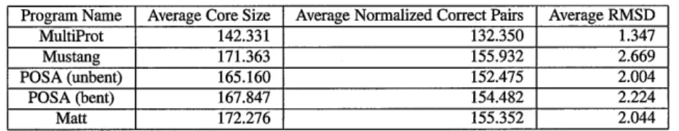
Program Name Average Core Size Average Normalized Correct Pairs Average RMSD MultiProt 142.331 132.350 1.347 Mustang 171.363 155.932 2.669 POSA (unbent) 165.160 152.475 2.004 POSA (bent) 167.847 154.482 2.224 Matt 172.276 155.352 2.044
Table 2.1: Homstrad performance comparison
2.3.3 Performance
Table 2.1 shows the following quantities for each program on the 399 Homstrad reference alignments that contain at least three structures each (this is the identical set of reference alignments on which POSA was tested). The first field is the average number of residues placed in the common core. The second is "average normalized correct pairs" computed according to the Homstrad reference alignments. This quantity is computed as follows: for each set of structures, we look at every pair of aligned residues that also participate in a Homstrad correct alignment. Then, we normalize based on the number of structures in the set (so the alignments in the set of 41 structures do not weight more heavily than the align-ments in the set of three structures), dividing by the number of pairs of distinct structures in the reference set. (Note that, as discussed in [60], having additional pairs placed into align-ment that Homstrad does not consider part of the "gold-standard" alignalign-ment is a positive, not a negative, if RMSD remains low. This is because declaring a pair of nearly aligned residues "aligned" or not is a judgment call that Homstrad makes partially based on older multiple structure alignment programs whose performance is weaker than the most recent programs.) The second column is the same "average RMSD" measure that POSA reports: the average RMS of the pairwise RMSDs among all pairs of residues that participate in a multiple alignment in a set of structures.
We downloaded and ran MultiProt and Mustang and computed RMSD statistics our-selves. POSA is only accessible as a web server; however, Homstrad alignments are available online at http://fatcat.bumham.org/POSA/POSAvsHOM.html. POSA's website provides two sets of multiple alignments: one derived from running their algorithm allow-ing geometrically impossible bends, and one runnallow-ing an unbent version of their algorithm. Note that for POSA's bent alignments, we had to recalculate RMSD from the multiple
se-2.8 2.7 2.6 2.5 2.1 2 80 85 90 95 100 105 Aligned residues
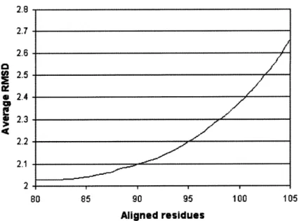
Figure 2-2: Matt SABmark performance tradeoff
Average pairwise RMSD versus average number of residue positions placed in the common core.
quence alignment provided from their bent alignments, because unbent RMSD based on bent alignments was not provided on their website. It is of independent interest that, as expected, POSA's unbent version has better RMSD, while POSA's bent version finds more residues participating in the alignments overall.
Matt scores slightly better than POSA on Homstrad. Matt's average core size is com-parable with that of Mustang, but Matt has a lower RMSD. The size of the alignments that MultiProt finds are much smaller than for the other programs (though its average RMSD is therefore much lower): this becomes even more pronounced on the more distant structures in SABmark (see Figure 2-2). Note that the core-size/RMSD tradeoff of Matt is very sen-sitive to cutoffs set in the last pass of the Matt algorithm, when it is decided what segments of less than five consecutive residues are added back into the alignment. Throughout this paper, the results reported in our tables come from setting the cutoff at 5
A.
By compari-son, if the cutoff is set at 3.5A,
Matt achieves 168.038 average core size, 153.362 average normalized pairs correct, and 1.862 average RMSD on Homstrad. Full tradeoff results on RMSD versus number of residues based on changing the last pass cutoff appear in Fig-ure 2-3. Note that Matt's cutoffs for allowable bends were trained on a random 20% of the Homstrad dataset.
2-t1.7
150 155 160 165 170 175
Aligned residues
Figure 2-3: Matt Homstrad performance tradeoff
Average pairwise RMSD versus average number of residue positions placed in the common core
Program Name Average Core Size Average RMSD
MultiProt 68.701 1.498
Mustang 104.162 4.146
Matt 104.692 2.639
Table 2.2: SABmark superfamily performance comparison
Program Name Average Core Size Average RMSD
MultiProt 36.354 1.536
Mustang 66.833 5.035
Matt 66.967 2.916
While Matt competes favorably with the other programs on Homstrad, Matt was de-signed for sets of more distantly related proteins than appear in the Homstrad benchmark. Thus, the best demonstration of the advantage of the Matt approach appears on the more distantly related proteins in the SABmark benchmark sets. Here, Matt is seen to do exactly what was hoped: by detouring through bent structures, it finds rigid RMSD alignments that place as many residues in the conserved alignment as Mustang does (and more than 50% more than MultiProt does) while reducing the average RMSD from that of Mustang by more than 1.4
A
(see Tables 2.2 and 2.3). It should again be emphasized that none of Matt's parameters were trained on SABmark.Looking by hand through the alignments, MultiProt consistently aligns small subsets of residues correctly, but leaves large regions unaligned that both Mustang and Matt believe to be alignable. Mustang, on the other hand, frequently misaligns regions, particularly in the case when there are many alpha-helices tightly packed in the structure. On two of the twilight zone sets, Mustang fails to find anything in the common core. Altogether on the twilight zone set, there are four sets of structures for which Mustang fails to find at least three residues in the common core (and there is one set of structures in the superfamily set where Mustang also fails to find anything in the common core). Though the effect is negligible, these four sets are removed from Mustang's average RMSD calculation.
Although these tables show overall performance, it is also helpful to look at actual examples. We pulled two example reference sets out of the SABmark superfamily bench-mark. Figure 2-4 shows the Matt alignment versus MultiProt, POSA, and Mustang align-ments of the SABmark structures in the set labeled Group 137 (beta-propellers; PDB IDs dlnr0al, dlnr0a2, d1p22a2, and dltbga). POSA does second best to Matt here, and in fact, the overall alignment of the structures in POSA is most similar to Matt- the same propeller blades are overlaid in both alignments. Although it is hard to see in the picture, Mustang is superimposing the wrong blades, which accounts for the terrible RMSD. MultiProt makes a similar error, but then gets a low RMSD by aligning less of the structure. Figure 2-5 shows a Matt alignment of the SABmark structures in the set labeled Group 144 (beta-helices; PDB IDs dlhm9al, dlkk6a, dlkrra, dllxa, dlocxa, dlqrea, dlxat, and d3tdt). Here, POSA does very poorly, only finding a very small set of residues to align. MultiProt again aligns
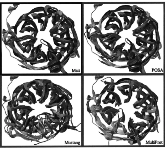
Figure 2-4: Comparative beta-propeller alignment
The four SABmark domains in the set Group 137, consisting of seven-bladed beta-propellers as aligned by POSA, Mustang, MultiProt, and Matt. Backbone atoms that participate in the common core of the alignment show up colored as red (PDB ID dlnr0al), green (PDB ID dlnr0a2), blue (PDB ID dlp22a2), and magenta (PDB ID dltbga); residues in all four chains that are not placed into the alignment by the tested algorithm are shown in gray. These pictures were generated by the Swiss PDB Viewer (DeepView) [38].
the portion that it declares in the common core very tightly (this is a theme throughout the SABmark dataset), but it only places five rungs in the common core. Both these fig-ures were generated using the Swiss PDB Viewer (DeepView) [38]. Core size and RMSD comparisons on both these reference sets appear in Table 2.4.
We then turn to the discrimination problem. Matt, FlexProt, Mustang, and MultiProt were tested on the SABmark superfamily and SABmark twilight zone decoy test suites described in the previous section. Using a method similar to what Gerstein and Levitt [34] did to systematically assess structure alignment programs against a gold standard, length of alignment versus RMSD for the true positives and true negatives were plotted in the plane
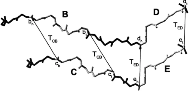
Figure 2-5: Comparative beta-helix alignment
Aligned portions of the eight SABmark domains in the set Group 144, consisting of the left-handed beta-helix fold as aligned by POSA, Mustang, MultiProt, and Matt. Backbone atoms that participate in the common core of the alignment show up colored as red (PDB ID dlhm9al), green (PDB ID dlkk6a), blue (PDB ID dlkrra), magenta (PDB ID dllxa), yellow (PDB ID dlocxa), orange (PDB ID dlqrea), cyan (PDB ID dlxat), and pink (PDB ID d3tdt); residues in all three chains that are not placed into the alignment by the tested algorithm are shown in gray. These pictures were generated by the Swiss PDB Viewer (DeepView) [38].
Propeller Core Size 180 218 252
261
Propeller RMSD Beta-Helix Core Size
1.73 79 6.13 83 2.62 23 2.35 98 Beta-helix RMSD 1.01 7.05 3.13 2.42
Table 2.4: Sample multiple structure alignments from SABmark benchmark
Program Name MultiProt Mustang POSA Matt _ I L __ __
M.a. t... FI.exFt
S0 .I
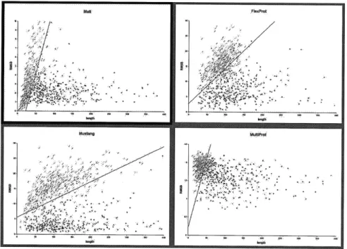
Figure 2-6: Distinguishing alignable structures from decoys
Positive (blue) and SABmark decoy (red) pairwise alignments plotted by RMSD versus number of residues for Matt, FlexProt, MultiProt, and Mustang on the SABmark superfamily set.
for all programs. Figure 2-6 displays the results on the SABmark superfamily set versus SABmark decoys. The separating line marks where the true positive and true negative percentages are roughly equal.
When comparing ROC curves over the four different programs, we find that Matt con-sistently dominates both FlexProt and MultiProt at almost every fixed true positive rate. Mustang does as well. Interestingly, Matt and Mustang are incomparable- on the Super-family sets, Matt does better than Mustang when the true positive rate is fixed over 93% (90% for the random decoy set), and Mustang does better thereafter. For the twilight zone set, the situation is reversed: SABmark does better than Matt when the true positive rate is between 93% and 98%, but Matt does better between 70% and 92% true positives; then, performance reverses, and Mustang does better below 70% true positive rates. Sample percentages for the four programs near the line where the true positive and true negative percentages are roughly equal appear in Tables 5 and 6 on the superfamily and twilight zone family sets, respectively.
Unsurprisingly, for all four programs, the SABmark decoy set was more difficult to
'VOL. .$~Wwai
41 4
I -- - --- -- - --- --- - --- --- - ~ I I
p:*-~ '- ' ir t:t '":Q''
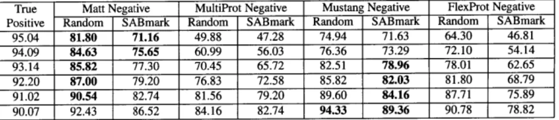
True Matt Negative MultiProt Negative Mustang Negative FlexProt Negative Positive Random SABmark Random SABmark Random SABmark Random SABmark
95.04 81.80 71.16 49.88 47.28 74.94 71.63 64.30 46.81 94.09 84.63 75.65 60.99 56.03 76.36 73.29 72.10 54.14 93.14 85.82 77.30 70.45 65.72 82.51 78.96 78.01 62.65 92.20 87.00 79.20 76.83 72.58 85.82 82.03 81.80 68.79 91.02 90.54 82.74 81.56 79.20 89.60 84.16 87.71 75.89 90.07 92.43 86.52 84.16 82.74 94.33 89.36 90.78 78.82
Table 2.5: Discrimination performance on the SABmark superfamily set
True negative percentage correct on the multiple structure alignment programs at a fixed true positive per-centage rate in the range close to where the true positive and true negative rates are equal. Results in bold are the best at that fixed true positive rate.
True Matt Negative MultiProt Negative Mustang Negative FlexProt Negative Positive Random SABmark Random SABmark Random SABmark Random SABmark
85.17 85.65 83.73 71.29 70.81 77.99 77.03 78.47 67.94 84.21 88.52 84.21 74.16 73.68 78.95 77.51 80.38 69.86 83.25 89.95 85.17 74.64 74.16 80.86 78.47 80.86 70.33 82.30 90.43 86.12 76.08 75.12 81.34 78.95 81.82 72.73 81.34 90.91 86.12 77.03 75.60 82.30 80.38 82.30 73.68 80.38 92.34 87.56 77.03 76.56 84.69 81.82 82.30 73.68
Table 2.6: Discrimination performance on the SABmark twilight zone set
True negative percent correct on the multiple structure alignment programs on the more difficult SABmark twilight zone set at a fixed true positive percentage rate, in the range close to where the two rates are equal. Results in bold are the best at that fixed true positive rate. Matt is always the best in this range.
classify than the random decoy set. What was more surprising is how competitive Mustang is with Matt on the discrimination tasks- it is surprising because Mustang was uniformly worse at the alignment problem. In essence, Mustang produces alignments with very high RMSD, but consistently even higher RMSD on the decoy sets. We hypothesize that this
may be due to Mustang's use of contact maps, a global measure of fold-fit that may be harder for decoys to match, whereas the decoys may have long regions of local
similar-ity. Matt and Mustang both do qualitatively better at all discrimination tasks than either MultiProt or FlexProt.
Note that in Figure 2-6 and in both Tables 2.5 and 2.6 we have used the RMSD of the best rigid-body transformation that matches the bent Matt or FlexProt alignment. At first, we hypothesized that the bent RMSD values might give better discrimination; after all, the bent structures are the local pieces that align really well. However, giving credit for the lower bent RMSD values also greatly improved the RMSD values for the decoy structures, leading in every case to worse performance on the discrimination tasks. Thus, reporting