A comparative study of techniques for protein side-chain placement

A Comparative Study of Techniques for Protein

Side-chain Placement

by

Eun-Jong Hong

B. S., Electrical Engineering

Seoul National University

(1998)

Submitted to the Department of Electrical Engineering and

Science

MASSACHUSETTS INSTITUTE OF TECHNOLOGY

OCT 1 5

2003

LIBRARIES Computer

in partial fulfillment of the requirements for the degree of

Master of Science in Electrical Engineering and Computer Science

at the

MASSACHUSETTS INSTITUTE OF TECHNOLOGY

September 2003

©

Massachusetts Institute of Technology 2003. All rights reserved.

A uthor ... ...

...

Department of Electrical Engineering and Computer Science

September 2, 2003

C ertified by ..

...

Tomas Lozano-Perez

Professor

T7hesis Supervisor

Accepted by....

Arthur C. Smith

Chairman, Department Committee on Graduate Students

A Comparative Study of Techniques for Protein Side-chain

Placement

by

Eun-Jong Hong

Submitted to the Department of Electrical Engineering and Computer Science on September 2, 2003, in partial fulfillment of the

requirements for the degree of

Master of Science in Electrical Engineering and Computer Science

Abstract

The prediction of energetically favorable side-chain conformation is a fundamental element in homology modeling of proteins and the design of novel protein sequences. The space of side-chain conformations can be approximated by a discrete space of probabilistically representative side-chain orientations (called rotamers). The prob-lem is, then, to find a rotamer selection for each amino acid that minimizes a potential function. This problem is an NP-hard optimization problem. The Dead-end elimi-nation (DEE) combined with the A* algorithm has been successfully applied to the problem. However, DEE fails to converge for some classes of complex problems.

In this research, we explore three different approaches to find alternatives to

DEE/A* in solving the GMEC problem. We first use integer programming

formu-lation and the branch-and-price algorithm to obtain the exact solution. There are known ILP formulations that can be directly applied to the GMEC problem. We re-view these formulations and compare their effectiveness using CPLEX optimizers. At the same time, we do a preliminary work to apply the branch-and-price to the GMEC problem. W suggest possible decomposition schemes, and assess the feasibility of the decomposition schemes by a computational experiment.

As the second approach, we use nonlinear programming techniques. This work mainly relies on the continuation approach by Ng [31]. Ng's continuation approach finds a suboptimal solution to a discrete optimization problem by solving a sequence of related nonlinear programming problems. We implement the algorithm and do a computational experiment to examine the performance of the method on the GMEC problem.

We finally use the probabilistic inference methods to infer the GMEC using the energy terms translated into probability distributions. We implement probabilistic re-laxation labeling, the max-product belief propagation (BP) algorithm, and the MIME double loop algorithm to test on side-chain placement examples and some sequence design cases. The performance of the three methods are also compared with the ILP method and DEE/A*.

the max-product BP algorithm is most effective and fast among all the tested meth-ods. Though the max-product BP algorithm is an approximate method, its speed and accuracy are comparable to those of DEE/A* in side-chain placement, and overall su-perior in sequence design. Probabilistic relaxation labeling shows slightly weaker per-formance than the max-product BP, but the method works well up to medium-sized cases. On the other hand, the ILP approach, the nonlinear programming approach, and the MIME double loop algorithm turns out to be not competitive. Though the three methods have different appearances, they are all based on the mathematical for-mulation and optimization techniques. We find such traditional approaches require good understanding of the methods and considerable experimental efforts and exper-tise. However, we also present the results from these methods to provide reference for future research.

Thesis Supervisor: Tomas Lozano-Perez Title: Professor

Acknowledgments

I would like to thank my advisor, Prof. Tomas Lozano-Perez, for his kind guidance and continuous encouragement. Working with him was a great learning experience and taught me the way to do research. He introduced me to the topic of side-chain placement as well as computational methods such as integer linear programming and probabilistic inference. He has been so much involved in this work himself, and most of ideas and implementations in Chapter 4 are his contributions. Without his hands-on advice and chands-onsiderate mentorship, this work was not able to be finished.

I also would like to thank Prof. Bruce Tidor and members of his group. Prof.

Tidor allowed me to access the group's machines, and use protein energy data and the DEE/A* implementation. Alessandro Senes, who used to be a post-Doc in the

Tidor group helped setting up the environment for my computational experiments. I appreciate his friendly responses to my numerous requests and answers to elemen-tary chemistry questions. I thank Michael Altman and Shaun Lippow for providing sequence design examples and providing helps in using their programs, Bambang Adi-wijaya for the useful discussion on delayed column generation.

I thank Prof. Piotr Indyk and Prof. Andreas Schultz for their helpful correspon-dence and suggestions on the problem, Prof. James Orlin and Prof. Dimitri Bertsekas for their time and opinions. Junghoon Lee was a helpful source on numerical meth-ods, and Yongil Shin became a valuable partner in discussing statistical physics and probability. Prof. Ted Ralphs of Lehigh University and Prof. Kien-Ming Ng of NUS gave helpful comments on their software and algorithm.

Last but not least, I express my deep gratefulness to my parents and sister for their endless support and love that sustain me throughout all the hard work.

Contents

1 Introduction

1.1 Global minimum energy conformation ...

1.1.1 NP-hardness of the GMEC problem . . . .

1.1.2 Purpose and scope . . . . 1.2 Related work . . . . 1.2.1 Integer linear programming (ILP) . . . . . 1.2.2 Probabilistic methods . . . .

1.3 Our approaches . . . . 2 Integer linear programming approach

2.1 ILP formulations . . . . 2.1.1 The first classical formulation by Eriksson, 2.1.2 The second classical formulation . . . .

2.1.3 The third classical formulation . . . . 2.1.4 Computational experience . . . . 2.2 Branch-and-price . . . . 2.2.1 Formulation . . . . 2.2.2 Branching and the subproblem . . . . 2.2.3 Implementation . . . . 2.2.4 Computational results and discussions . . 2.3 Sum m ary . . . . 11 11 12 13 14 14 14 15 17 . . . . 17

Zhou, and Elofsson 17 . . . . 19 . . . . 20 . . . . 2 1 . . . . 23 . . . . 23 . . . . 3 1 . . . . 32 . . . . 35 . . . . 39

3 Nonlinear programming approach

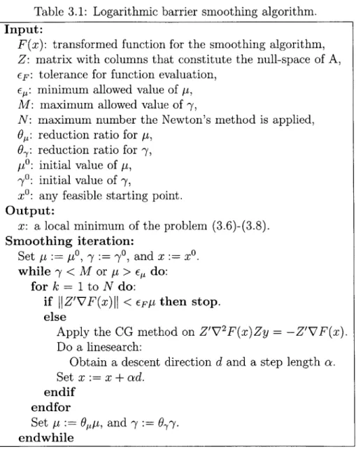
3.1 Ng's continuation approach ...

3.1.1 Continuation method ...

3.1.2 Smoothing algorithm . . . .

3.1.3 Solving the transformed problem . . . .

3.2 Algorithm implementation . . . . 3.2.1 The conjugate gradient method . . . .

3.2.2 The adaptive linesearch algorithm. . . . .

3.3 Computational results . . . .

3.3.1 Energy clipping and preconditioning the reduced-Hessian

3.3.2 Parameter control and variable elimination . . . .

3.3.3 R esults . . . . 3.4 Sum m ary . . . .

4 Probabilistic inference approach

4.1 M ethods . . . .

4.1.1 Probabilistic relaxation labeling 4.1.2 BP algorithm . . . . 4.1.3 Max-product BP algorithm . . 4.1.4 Double loop algorithm . . . . . 4.1.5 Implementation . . . . 4.2 Results and discussions . . . . 4.2.1 Side-chain placement . . . . 4.2.2 Sequence design . . . . 4.3 Summary . . . .

5 Conclusions and future work

41 . . . 42 . . . 42 . . . 42 . . . 45 . . . 48 . . . 48 . . . 48 50 system 53 . . . 53 . . . 55 58 60 . . . . 6 0 . . . . 6 1 . . . . 6 1 . . . . 6 2 . . . . 6 3 . . . . 6 4 . . . . 6 5 . . . . 6 5 . . . . 7 4 . . . . 7 6 77

List of Figures

2-1 Problem setting . . . . 25

2-2 A feasible solution to the GMEC problem . . . . 26

2-3 A set of minimum weight edges . . . . 26

2-4 Path starting from rotamer 2 of residue 1 and arriving at the same rotam er . . . . 27

2-5 An elongated graph to calculate shortest paths . . . . 28

2-6 Fragmentation of the maximum clique . . . . 29

4-1 An example factor graph with three residues . . . . 62

4-2 The change in the estimated entropy distribution from MP for lamm-80. 71 4-3 The change in the estimated entropy distribution from MP for 256b-80. 72 4-4 Histogram of estimated entropy for lamm-80 and 256b-80 at conver-gence of M P . . . . . 72

List of Tables

2.1 Comparison of three classical formulations (protein: PDB code, #res:

number of modeled residues, LP solution: I - integral, F - fractional,

TLP: time taken for CPLEX LP Optimizer, Tip: time taken for

CPLEX MIP Optimizer, symbol - : skipped, symbol * : failed). . . . 22

2.2 Test results for BRP1 (IS*I: total number of feasible columns, #nodes: number of explored branch-and-bound nodes, #LP: number of solved LPs until convergence, #cols: number of added columns until conver-gence, (frac): #cols to IS*1 ratio, #LPop: number of solved LPs until reaching the optimal value, #colsop: number of added columns until reaching the optimal value, TLP: time taken for solving LPs in seconds,

Taub: time taken for solving subproblems in seconds, symbol - : IS*1

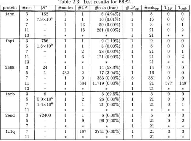
calculation overflow, symbol *: stopped while running). . . . . 37 2.3 Test results for BRP2. . . . . 38

2.4 Test result for BRP3. . . . . 38 2.5 Test results with random energy examples (#nodes: number of

ex-plored branch-and-bound nodes, LB: lower bound from LP-relaxation, T: time taken to solve the instance exactly, symbol * : stopped while running). . . . . 39 3.1 Logarithmic barrier smoothing algorithm . . . . 47

3.2 The preconditioned CG method for possibly indefinite systems. . . . . 49

3.4 The parameter settings used in the implementation. . . . . 55 3.5 Results for SM2. (protein: PDB code, #res: number of residues, #var:

number of variables, optimal: optimal objective value, smoothing: ob-jective value from the smoothing algorithm, #SM: number of smooth-ing iterations, #CG: number of CG calls, time: execution time in sec-onds, #NC: number of negative curvature directions used, -0: initial

value of the quadratic penalty parameter.) . . . . 56 3.6 Results for SM1. . . . . 58

4.1 The protein test set for the side-chain placement (logloconf: log total conformations, optimal: optimal objective value, TLP: LP solver

solu-tion time, TIp: IP solver solusolu-tion time, TDEE: DEE/A* solution time,

symbol - : skipped case, symbol * : failed, symbol F : fractional LP

solution). . . . . 67

4.2 Results for the side-chain placement test (AE: the difference from the optimal objective value, symbol - : skipped). . . . . 69

4.3 The fraction of incorrect rotamers from RL, MP, and DL. . . . . 69

4.4 Performance comparison of MP and DEE/A* on side-chain placement (optimal: solution value from DEE/A*, EMP: solution value from MP,

AE: difference between 'optimal' and EMp, IRMp: number of

incor-rectly predicted rotamers by MP, TDEE: time taken for DEE/A* in

seconds, TMp: time taken for MP in seconds). . . . . 70

4.5 Fraction of incorrectly predicted rotamers by MP and statistics of the estimated entropy for the second side-chain placement test. (IR frac-tion: fraction of incorrectly predicted rotamers, avg Si: average es-timated entropy, max Si: maximum eses-timated entropy, min Si: mini-mum estimated entropy, miniEIR Si: minimum entropy of incorrectly

predicted rotam ers). . . . . 73

4.6 The protein test set for sequence design (symbol ? : unknown optimal value, symbol * : failed). . . . . 75

4.7 Results for sequence design test cases whose optimal values are known. 75

4.8 Results for sequence design test cases whose optimal values are un-known (E: solution value the method obtained). . . . . 75

Chapter 1

Introduction

1.1

Global minimum energy conformation

The biological function of a protein is determined by its three-dimensional (3D) struc-ture. Therefore, an understanding of the 3D structures of proteins is a fundamental element in studying the mechanism of life. The widely used experimental techniques for determining the 3D structures of proteins are X-ray crystallography and NMR spectroscopy, but their uses are difficult and sometimes impossible because of the high cost and technical limits. On the other hand, the advances in genome sequenc-ing techniques have produced an enormous number of amino-acid sequences whose folded structures are unknown. Researchers have made remarkable achievements in exploiting the sequences to predict the structures computationally. Currently, due to the increasing number of experimentally known structures and the computational prediction techniques such as threading, we can obtain approximate structures corre-sponding to new sequences in many cases. With this trend, we expect to be able to have approximate structures for all the available sequences in the near future.

However, approximate structures are not useful enough in many practical pur-poses, such as understanding the molecular mechanism of the protein, or designing an amino-acid sequence compatible with a given target structure. Homology model-ing of proteins [7] and design of novel protein sequences [6] are often based on the prediction of energetically favorable side-chain conformations. The space of side-chain

conformations can be approximated by a discrete space of probabilistically represen-tative side-chain orientations (called rotamers) [34].

The discrete model of the protein energy function we use in this work is described in terms of:

1. the self-energy of a backbone template (denoted as ebackbone)

2. the interaction energy between the backbone and residue i in its rotamer con-formation r in the absence of other free side-chains (denoted as ei,)

3. the interaction energy between residue i in the rotamer conformation r and residue j in the rotamer conformation s, i = j (denoted as eir.j)

In the discrete conformation space, the total energy of a protein in a specific confor-mation C can be written as follows:

Sc = C-ackbone +

i

ei, + ej. (1.1

2 i j>i

The problem is, then, to find a rotamer selection for the modeled residues that min-imizes the energy function Sc, which is often called global minimum energy confor-mation (GMEC). In this work, we call the problem as the GMEC problem.

1.1.1

NP-hardness of the GMEC problem

The GMEC problem is a hard optimization problem. We can easily see that it is equivalent to the maximum capacity representatives (MCR), a NP-hard optimization problem. A Compendium of NP optimization problems by Crescenzi [5] describes the MCR as follows:

Instance Disjoint sets Si, ... , Sm and, for any i

#

j, x C Si, and y C Si, a

nonneg-ative capacity c(x, y).

Solution A system of representatives T, i.e., a set T such that, for any i, JTnSi = 1. Measure The capacity of the system of representatives, i.e., ExyET c(x, y).

To reduce the MCR to the GMEC problem, we regard each set Si as a residue and its elements as the residue's rotamers. Then, we take the negative value of the capacity between two elements in two different sets as the interactive energy between corresponding rotamers and switch the maximization problem to a minimization prob-lem. This is a GMEC problem with ej, equal 0 for all i and r. A rigorous proof of

NP-hardness of the GMEC problem can be found in [38].

As illustrated by the fact that the GMEC problem is an NP-hard optimization problem, the general form of the GMEC problem is a challenging combinatorial prob-lem that have many interesting aspects in both theory and practice.

1.1.2

Purpose and scope

Our purpose of the study is generally two-fold. First, we aim to find a better method to solve the GMEC problem efficiently. Despite the theoretical concept of hardness, we often find many instances of the GMEC problem are easily solved by exact methods such as Dead-End Elimination (DEE) combined with A* (DEE/A*) [8, 26]. However, DEE's elimination criteria are not always powerful in significantly reducing the prob-lem's complexity. Though there have been modifications and improvements over the original elimination conditions [12, 33, 11], the method is still not quite a general solution to the problem, especially in the application of sequence design. In this work, we explore both analytical and approximate methods through computational experiments. We compare their performance with one another to identify possible alternatives to DEE/A*. There exists a comparative work by Voigt et al. [40], which examines the performance of DEE with other well-known methods such as Monte Carlo, genetic algorithms, and self-consistent mean-field that concludes DEE is the the most feasible method. We intend to investigate new approaches that have not been used or studied well, but have good standings as appropriate techniques for the

GMEC problem.

In the second place, we want to understand the working mechanism of the meth-ods. There are methods that are not theoretically understood well, but show extraor-dinary performance in practice. On the other hand, some methods are effective only

for a specific type of instances. For example, the belief propagation and LP approach are not generally good solutions to the GMEC problem with random artificial energy terms, but they are very accurate for the GMEC instances with protein energy terms. Our ultimate goal is to be able to explain why or when a specific method succeeds and fails.

The scope of this work is mainly computational aspects of the side-chain place-ment problem using rotamer libraries. Therefore, we leave issues such as protein energy models, and characteristics of rotamer libraries out of our work.

1.2

Related work

1.2.1

Integer linear programming (ILP)

The polyhedral approach is a popular technique for solving hard combinatorial opti-mization problems. The main idea behind the technique is to iteratively strengthen the LP formulation by adding violated valid inequalities.

Althaus et al. [1] presented an ILP appraoch for side-chain demangling in rotamer representation of the side chain conformation. Using an ILP formulation, they iden-tified classes of facet-defining inequalities and devised a separation algorithm for a subclass of inequalities. On average, the branch-and-cut algorithm was about five times slower than their heuristic approach.

Eriksson et al. [9] also formulated the side chain positioning problem as an ILP problem. However, in their computational experiments, they found that the LP-relaxation of every test instance has an integral solution and, therefore, the integer programming (IP) techniques are not necessary. They conjecture that the GMEC problem always has integral solutions in LP-relaxation.

1.2.2

Probabilistic methods

A seminal work using the self-consistent mean field theory was done by Koehl and

energy weighted by the conformational probabilities. The conformational probabil-ities are related to the mean field energy by the Boltzmann law. Iterative updates of the probabilities and the mean field energy are performed until they converge. At convergence, the rotamer with the highest probability from each residue is selected as the conformation. The method is not exact, but has linear time complexity.

Yanover and Weiss [42] applied belief propagation (BP), generalized belief propa-gation (GBP), and mean field method to finding minimum energy side-chain configu-ration and compared the results with those from SCWRL, a protein-folding program. Their energy function is approximate in that local interactions between neighboring residues are considered, which results in incomplete structures of graphical models. The energies found by each method are compared with those from one another, rather than with optimal values from exact methods.

1.3

Our approaches

In this research, we use roughly three different approaches to solve the GMEC prob-lem. In Chapter 2, we use integer programming formulation and the branch-and-price algorithm to obtain exact solutions. There are known ILP formulations that can be directly applied to the GMEC problem. We review these formulations and compare their effectiveness using CPLEX optimizers. At the same time, we do a preliminary work to apply the branch-and-price to the GMEC problem. We review the algorithm, suggests possible decomposition schemes, and assess the feasibility of the decomposi-tion schemes by a computadecomposi-tional experiment.

As the second approach, we use nonlinear programming techniques in Chapter 3. This work mainly relies on the continuation approach by Ng [31]. Ng's continuation approach finds a suboptimal solution to a discrete optimization problem by solving a sequence of related nonlinear programming problems. We implement the algorithm and do a computational experiment to examine the performance of the method on the GMEC problem.

the energy terms translated into probability distributions. We implement probabilis-tic relaxation labeling, the max-product belief propagation (BP) algorithm, and the MIME double loop algorithm to test on side-chain placement examples as well as some sequence design cases. The performance of the three methods are also com-pared with the ILP method and DEE/A*.

The preliminary results suggest that probabilistic inference methods, especially the max-product BP algorithm is most effective and fast among all the tested meth-ods. Though the max-product BP algorithm is an approximate method, its speed and accuracy are comparable to those of DEE/A* in side-chain placement, and overall su-perior in sequence design. Probabilistic relaxation labeling shows slightly weaker per-formance than the max-product BP, but the method works well up to medium-sized cases. On the other hand, the ILP approach, the nonlinear programming approach, and the MIME double loop algorithm turns out to be not competitive. Though the three methods have different appearances, they are all based on the mathematical for-mulation and optimization techniques. We find such traditional approaches require good understanding of the methods and considerable experimental efforts and exper-tise. However, we also present the results from these methods to provide reference

Chapter 2

Integer linear programming

approach

In this chapter, we describe different forms of integer linear programming (ILP) for-mulations of the GMEC problem. We first present a classical ILP formulation by Erkisson et al., and two similar formulations adopted from related combinatorial optimization problems. Based on these classical ILP formulations, we review the mathematical notion of the branch-and-price algorithm and consider three different decomposition schemes for the column generation. Finally, some preliminary results from implementations of the branch-and-price algorithm are presented.

2.1

ILP formulations

2.1.1

The first classical formulation by Eriksson, Zhou, and

Elofsson

In the ILP formulation of the GMEC problem by Eriksson et al. [9], the self-energy of each rotamer is evenly distributed to every interaction energy involving the tamer. A residue's chosen rotamer interacts with every other residue's chosen ro-tamer. Therefore, the self-energies can be completely incorporated into the interac-tion energies without affecting the total energy by modifying the interacinterac-tion energies

as follows:

e' = ei, + ej, (2.1)

n- I

where n is the number of residues in the protein. Then, the total energy of a given conformation C can be written as

Sc = Z e'g. (2.2)

i j>i

Since the total energy now only depends on the interaction energy, Ec can be expressed as a set of value assignments on binary variables that decide whether an interaction between two residues in a certain conformation exists or not. We let xijs, be a binary variable, where its value is 1 if residue i is in the rotamer conformation r, and residue j is in the rotamer conformation s, and 0 otherwise. We also let Ri denote the set of all possible rotamers of residue i. Then, the total energy in conformation

C is given by

c=

S S S S

e' xijs. (2.3)

i _{rERj j>i sERj}

On the other hand, there should exist exactly one interaction between any pair of residues. Therefore, we have the following constraints on the value of xigj,:

E E xijs = for all i and j, i < j. (2.4)

rERj sERj

Under the constraint of (2.4), more than one rotamer can be chosen for a residue. To make the choice of rotamers consistent throughout all residues, we need the following

constraints on xir i:

Xhq . = Xgpr = xjr Xikt (2.5)

qERh pERg SERj tERk

(2.6)

Finally, by adding the integer constraints

X'js E {0, 1}, (2.7)

we have an integer programming that minimizes the cost function (2.3) under the

constraints (2.4) - (2.7). We denote (2.3) - (2.7) by Fl.

Eriksson et al. devised this formulation to be used within the framework of integer programming algorithms, but they found that the LP relaxation of this formulation always has an integral solution and hypothesized that every instance of the GMEC problem can be solved by linear programming. However, in our experiments, we found some instances have fractional solution to the LP relaxation of F1, which is not sur-prising since the GMEC problem is an NP-hard optimization problem. Nonetheless, except two cases, all solved LP relaxations of F1 had integral solutions.

2.1.2

The second classical formulation

Here, we present the second classical ILP formulation of the GMEC problem. This is a minor modification of the formulation for the maximum edge-weighted clique problem (MEWCP) by Hunting et al. [17]. The goal of the MEWCP is to find a clique with the maximum sum of edge weights.

If we take a graph theoretic approach to the GMEC problem, we can model each rotamer r for residue i as a node ir, and the interaction between two rotamers r and

s for residues i and j, respectively, as an edge (ir, js). Then, the GMEC problem

reduces to finding the minimum edge-weighted maximum clique of the graph.

We introduce binary variables xi, for node i, for all i and r C Ri. We also adopt binary variables yijj for each edge (ir, Js) for all i and j, and for all r E Ri and S E R. Variable xi, takes value 1 if node ir is included in the selected clique, and 0 otherwise. Variable yij, takes value 1 if edge (ir,

js)

is in the clique, and 0 otherwise. We define V and E as follows:

E = {(zr, js)I V ZrJ E V}. (2.9)

Then, the adapted ILP formulation of the MEWCP is given by

min E eirxi, + E eirjsyirjs (2.10)

irEV (ir,j.)EE

yir, - Wir < 0, V(ir, js) E E, (2.11) Yirs - Xis < 0, V(ir,js) E E, (2.12)

Xir + Xj - 2Yijri j 0, V(ir, js) C E, (2.13)

Li, E {0, 1}, Vi, E V, (2.14)

Yirjs > 0, V(ir, js) E E. (2.15)

To complete the formulation of the GMEC problem, we add the following set of constraints, which implies that exactly one rotamer should be chosen for each residue:

E Xj, = 1. (2.16)

r ER

We denote (2.10) - (2.16) by F2. When the CPLEX MIP solver was used to solve

a given GMEC instance in both F1 and F2, F1 was faster than F2. This is mainly because F2 heavily depends on the integrality of variables xi,. On the other hand, F2 has an advantage when used in the branch-and-cut framework since polyhedral results and Lagrangean relaxation techniques are available for the MEWCP that can be readily applied to F2. [17, 28]

2.1.3

The third classical formulation

Koster et al. [25] presented another formulation that captures characteristics of two previous formulations. Koster et al. studied solution to the frequency assignment problem (FAP) via tree-decomposition. There are many variants of the FAP, and, in-terestingly, the minimum interference frequency assignment problem (MI-FAP)

stud-ied by Koster et al. has exactly the same problem setting as the GMEC problem, except that the node weights and edge weights of the MI-FAP are positive integers.

The formulation suggested by Koster et al. uses node variables and combines the two styles of constraints from the previous formulations. If we transform the problem setting of the FAP into that of the GMEC problem, we obtain the following ILP formulation for the GMEC problem:

min E eixi, +

3

eijsyij, (2.17)

iEV (irjs)EE

Z

Xi, = 1, (2.18)

r ER.

Syij,

= xi,, Vj # i, Vs E Ri, Vi, Vr E Ri, (2.19)

sERj

Xi, E {0, 1}, Vzr E V, (2.20)

YirjS > 0, V(ir, js) E E. (2.21)

We denote (2.17) - (2.21) by F3. In F3, (2.18) restricts the number of selected rotamers for each residue to one as it does in F2. On the other hand, (2.19) enforces that the selection of interactions should be consistent with the selection of rotamers. Koster et al. studied the polytope represented by the formulation, and developed facet defining inequalities [22, 23, 24].

2.1.4 Computational experience

We performed an experimental comparison of the classical ILP formulations F1, F2, and F3. The formulations were implemented in C code using CPLEX Callable Li-brary. The test cases of lbpi, lamm, larb, and 256b were generated using a common rotamer library (called by LIB1 throughout the work), but a denser library (LIB2) was used to generate test cases of 2end. The choice of modeled proteins followed the work by Voigt et al. [40]. We made several cases with different sequence lengths using the same protein to control the complexity of test cases. The energy terms were

Table 2.1: Comparison of three classical formulations (protein: PDB code, #res: number of modeled residues, LP solution: I - integral, F - fractional, TLP: time taken for CPLEX LP Optimizer, TIp: time taken for CPLEX MIP Optimizer, symbol -: skipped, symbol *

:

failed).

LP solution TLP (sec) Tip (sec)

protein #res F1 F2 F3 F1 F2 F3 F1 F3 lbpi 10 I F I 0 1 0 0 0 20 I F I 0 8 1 0 0 25 I F I 0 134 0 3 1 46 I F I 29 6487 14 37 16 1aMM 10 I F I 0 0 0 0 0 20 I F I 1 96 0 1 0 70 I F I 42 33989 29 45 48 80 I F I 97 * 69 99 102 larb 10 I I I 0 0 0 0 0 20 I F I 0 0 0 0 0 30 I F I 0 15 0 1 0 78 I F I 24 10384 21 27 25 256b 30 I - I 3 - 2 6 3 40 I - I 10 - 4 14 6 50 I - I 26 - 12 36 15 60 I - I 60 - 36 87 37 70 F - F 116 - 98 156 112 2end 15 I - I 31 - 35 34 41 25 I - I 281 - 214 343 240

calculated by the CHARM22 script. All experiment was done on a Debian worksta-tion with a 2.20 GHz Intel Xeon processor and 1 GBytes of memory. We used both CPLEX LP Optimizer and Mixed Integer Optimizer to compare the solution time between the formulations. The results are listed in Table 2.1.

The result from LP Optimizer tells that F2 is far less effective in terms of both the lower bounds it provides and the time needed for the LP Optimizer. F2 obtained only fractional solutions whereas F1 and F3 solved most of the cases optimally. F1 and F3 show similar performance though F3 is slightly more effective than F1 in LP-relaxation. Since F2 showed inferior performance in LP-relaxation, we measured Mixed Integer Optimizer's running time only with F1 and F3. As shown in the last two columns of Table 2.1, Mixed Integer Optimizer mostly took more time for F1

than F3, but no more than a constant factor as was the case with LP Optimizer. CPLEX optimizers were able to solve the small- to medium-sized cases, but us-ing the optimizers only with a fixed formulation turns out to be not very efficient.

On the other hand, DEE/A* is mostly faster than the CPLEX optimizers using the classical formulations, which makes the ILP approach entirely relying on general op-timizers look somewhat futile. We also observe cases that both F1 and F3 obtain fractional solutions in LP-relaxation while solving large IP's usually takes signifi-cantly more time than solving corresponding LP-relaxations. This suggests that we should explore the possible development of a problem specific IP solver that exploits the special structure of the GMEC problem. As an effort toward this direction, in Section 2.2, we investigate the possible use of the branch-and-price algorithm based on F1 formulation.

2.2

Branch-and-price

The branch-and-price (also known as column generation IP) is a branch-and bound algorithm that performs the bounding operation using LP-relaxation [3]. Particu-larly, the LP relaxation at each node of the branch-and-bound tree is solved using the delayed column generation technique. It is usually based on an IP formulation that introduces a huge number of variables but has a tighter convex hull in LP relaxation than a simpler formulation with fewer variables. The key idea of the method is split-ting the given integer programming problem into the master problem (MP) and the subproblem (SP) by Dantzig-Wolfe decomposition and then exploiting the problem specific structure to solve the subproblem.

2.2.1

Formulation

In this section, we first review the general notion of the branch-and-price formulation developed by Barnhart et al. [3] and devise appropriate Dantzig-Wolfe decomposition of F1.

The previous classical ILP formulations can be all captured in the following general form of ILP:

Ax < b,2

E S, x E {O, 1}", (2.24)

where c E Rn is a constant vector, and A is an m x n real-valued matrix. The basic idea of the Dantzig-Wolfe decomposition involves splitting the constraints into two separate sets of constraints - (2.23) and (2.24), and representing the set

S* = {XE S I XE {O,1}"} (2.25) by its extreme points. S* is represented by a finite set of vectors. In particular, if S is

bounded, S* is a finite set of points such that S* =

{yi,...

, yp }, where yi E R?, i =

,. . . , P .

Now, if we are given S* = {yi, ... , yP}, any point y E S* can be represented as

y =

Z

Ak, (2.26)

subject to the convexity constraint

S:

A k =1 (2.27)

1<k~p

Ak {O, 1}, k = 1, ... Ip. (2.28)

Let ck = c'yk, and ak = Ayk. Then, we obtain the general form of branch-and-price formulation for the ILP given by (2.22) - (2.24) as follows:

min E ck Ak (2.29) 1<k~p ak Ak < b, (2.30) 1<k<p E Ak 1, (2.31) 1<k= A k EE {0, 1}, k = 1, ... IpA (2.32) (2.23)

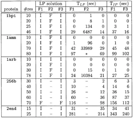
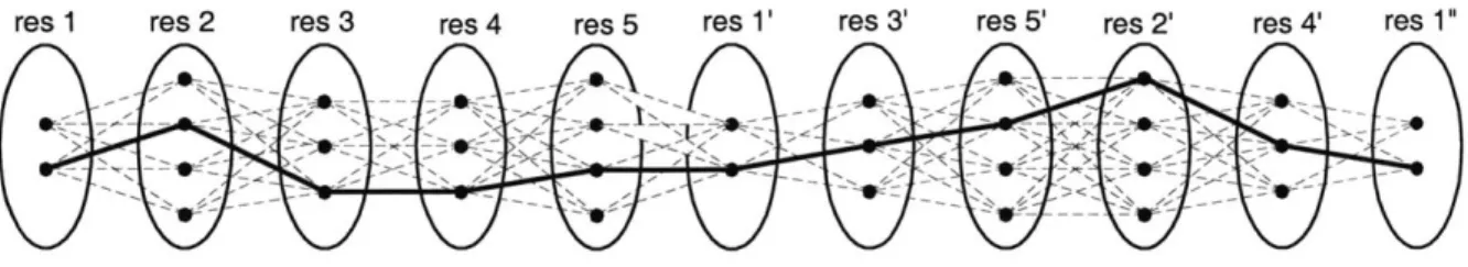
Figure 2-1: Problem setting

The fundamental difference between the classical ILP formulation (2.22) - (2.24) and the branch- and-price formulation (2.29) - (2.32) is that S* is replaced by a finite set of points. Moreover, any fractional solution to the LP relaxation of (2.22)

-(2.24) is a feasible solution of the LP relaxation of (2.29) - (2.32) if and only if the

solution can be represented by a convex combination of extreme points of conv(S*).

Therefore, it is easily inferred that the LP relaxation of (2.29) - (2.32) is at least as

tight as that of (2.22) - (2.24) and more effective in branch- and-bound.

Now we recognize that success of the branch-and-price algorithm will, to a great extent, depend on the choice of base formulation we use for (2.22) - (2.24) and how we decompose it. In this work, we use F1 as the base ILP formulation for it usually has the smallest number of variables and constraints among F1, F2, and F3, and also has good lower bounds. Designing the decomposition scheme is equivalent to defining S*. Naturally, the constraints corresponding to (2.23) will be the complement constraints

of S* in the (2.4) - (2.7).

We consider three different definitions of S* below.

Set of edge sets

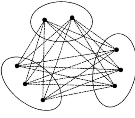
Figure 2-1 is a graphical illustration of the problem setting, and Figure 2-2 shows the feasible solution when all constraints are used. In fact, any maximum clique of the graph is a feasible solution. In this decomposition scheme, we consider only the

I If

-- --- % -'--

-Figure 2-2: A feasible solution to the GMEC problem

Figure 2-3: A set of minimum weight edges

constraint that one interaction is chosen between every pair of residues. Formally, we have

S* =

{Q

I Q is a set of (ir, js), Vr E R, Vs E R1, Vi, Vj}. (2.33) We denote this definition of S* by S1.

The subproblem is finding out the smallest weight edge between each pair of residues. A solution to the subproblem will generally look like Figure 2-3. The size of S1 is exponential to the original solution space, but each subproblem can be solved

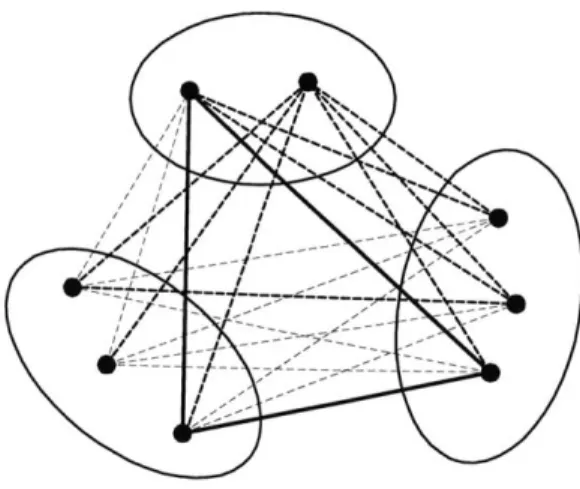
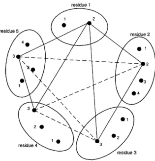
residue 1 2 residue 5 ₄ residue 4 3 2 2 10 03 0 4 3 01 2 residue 43 2 residue 3

Figure 2-4: Path starting from rotamer 2 of residue 1 and arriving at the same rotamer

Set of paths

We can define S* to be the set of paths that starts from node i, and arrives at the same node by a sequence of edges connecting each pair of residues as illustrated by Figure 2-4. A column generated this way is a feasible solution to the GMEC problem only if the number of visited rotamers at each residue is one. We denote S* defined

this way as S2.

The size of S2 is approximately the square root of the size of S1. In this case, the

subproblem becomes the shortest path problem if we replicate a residue together with its rotamers and add them to the path every time the residue is visited. Figure

2-5 shows how we can view the graph to apply the shortest path algorithm. The

subproblem is less simple than the case S* = S1, but we can efficiently generate

multiple columns at a time if we use the k-shortest path algorithm.

The inherent hardness of the combinatorial optimization problem is independent of the base ILP formulation or the decomposition scheme used in the branch-and-price algorithm. Therefore, the decomposition can be regarded as the design of the balance point between the size of S* and the hardness of the subproblem.

res 1 res 2 res 3 res 4 res 5 res 1' res 3' res 5' res 2' res 4' res1"

Figure 2-5: An elongated graph to calculate shortest paths

residue on the path but the first. To make the column generation more efficient, we can try fixing several residues' rotamers on the path as we do for the first residue. Set of cliques

Based on the idea of partitioning a feasible solution, or a maximum clique into small cliques, the third decomposition we consider is to define S3 as a set of cliques. Figure

2-6 illustrates this method. A maximum clique consisting of five nodes is fragmented

into two three-node cliques composed of nodes 12, 22, 33 and nodes 12, 33, 53 respec-tively. To complete the maximum clique, four edges represented by dashed lines are

added (an edge can be also regarded as a clique of two nodes.)

The branch-and-price formulation for this decomposition differs from (2.29) -(2.32) in that (2.31) and -(2.32) are not necessary. All the assembly of small cliques

are done by (2.30) and it is possible we obtain an integral solution when (2.29) -(2.32) has a fractional optimal solution from LP-relaxation. Therefore, the branching

is also determined by examining the integrality of original variables, x of (2.22)

-(2.24).

The size of S3 is obviously smaller than those of Si and S2. If we let n be the

number of residues, and m be the maximum number of rotamers for one residue, the

i Mn(n-1) 0( ~)

size of S2 is O(m 2 ). In comparison, the size of is S₃ O((m + 1)").

The subproblem turns out to be the minimum edge-weighted clique problem (MEWCP), which is an NP-hard optimization problem. Macambira and de Souza [28] have investigated the MEWCP with polyhedral techniques, and there is also an La-grangian relaxation approach to the problem by Hunting et al. [17]. However, it is more efficient to solve the subproblem by heuristics such as probabilistic relaxation

residue 1 12 residue 5 _{residue 2} 4 3 \ 2 30 2 40 residue 4 103 0 residue 3

Figure 2-6: Fragmentation of the maximum clique

labeling [32, 15, 16] that will be examined in Chapter 4 and use the analytical tech-niques only if heuristics fail to find any new column.

On the other hand, there exists a pitfall in application of this decomposition; by generating edges as columns, we may end up with the samebasis for the LP relax-ation of the base formulrelax-ation. To obtain a better lower bound, we need to find a

basis that better approximates the convex hull of integral feasible points than that of

the LP-relaxed base formulation. However, by generating edges as columns necessary

to connect the small cliques, the column generation will possibly converge only after

exploring the edge columns. One easily conceivable remedy is generating only cliques with at least three nodes, but it is a question whether this is a better decomposition

scheme in practice than, say, S* = S2.

The Held-Karp heuristic and the branch-and-price algorithm

Since we do not have separable structures in the GMEC problem, it seems more appropriate to first relax the constraints to generate columns and then to sieve them with the rest of the constraints by LP. Defining S* to be S2 is closer to this scheme than defining it to be S3. We show that this scheme is, in fact, compatible with

the idea behind the Held-Karp heuristic, and suggest that we should take a similar approach to develop an efficient branch-and-price algorithm for the GMEC problem. Let G be a graph with node set V and edge set E, and aij be the weight on the edge (i, j). Then, the traveling salesman problem (TSP) is often represented as

min E

Y

aijxij (2.34) xjzj = 1, Vi E V, (2.35) VjEVlj:Ai

Z

xjj = 1, Vj V. (2.36) ViGV,i=Aj (ij + x ji) ;> 2, VS C V, S # V, (2.37) ij= {0, 1}, V(i, j) E E. (2.38)

(2.35) and (2.36) are conservation of flow constraints. (2.37) is a subtour elimination

constraint [4]. In Held-Karp heuristic, (2.37) and (2.38) are replaced by

(V, {(i, j) I xij = 1}) is a 1-tree. (2.39) If we assign the Lagrangian multipliers u and v, the Lagrangian function is

L(x, u, v) = E (ai + ui + vj)xij - E ui - E j. (2.40)

i,jeV, i7j iEV jeV

Finally, if we let

S = {x I xij E {0, 1} such that (V, {(i,

j)

ij = 1}) is a 1-tree}, (2.41) the value produced by the Held-Karp heuristic is essentially the optimal dual value given by

q* = sup inf L(x, u,v). (2.42)

When the cost and the inequality constraints are linear, the lower bounds obtained

by Lagrangian relaxation and integer constraints relaxation are equal

[4].

Therefore, if S* is a finite set of points, say S* = yi ... yP}, y E RIE, J = 1,... ,p, the optimal value of the following LP is also q*:

mn aij E AkYk (2.43)

ViEV VjEVjfi I kip

Aky = 1, Vi C V, (2.44)

VjEV,jhi 1<kip

Akyk= 1, Vj E V, (2.45)

ViEV,ifj 1<k<p

Yk E S* O < Ak < 1 k = 1, ... ,p. (2.46) Note that (2.43) - (2.46) make a LP relaxation of the branch-and-price formulation of the original ILP, or simply a Dantzig-Wolfe decomposition. Thus, we confirm that the Held-Karp heuristic is essentially equivalent to the branch-and-price algorithm applied to the TSP.

2.2.2

Branching and the subproblem

For all decomposition schemes, we use branching on original variables. In other words, when the column generation converges for node U of the branch-and-bound tree and it is found that the LP-relaxation of the restricted master problem (RMP) at U has a fractional solution, we branch on a variable xi of (2.22) - (2.24) rather than on a variable Ak of (2.29) - (2.32). Formally, if we have the RMP for node U with the

form of (2.29) - (2.32), S is branched on xt to two nodes Uo and U1, where the RMP

at U is given by min ckAk (2.47) k:1 k~p, yk=i a A ak b, _(2.48) k:15ksp, yk~ Ak = 1, (2.49) k:1<k<p, yk=i

Ak E {0, 1}, k = 1,. .. , p. (2.50)

In our implementation, the branching variable xt is an edge variable for we use (2.3)

- (2.7) as the base formulation. The branch variable xt is determined by calculating the value of x from the fractional solution A and taking the one whose value is closest to 1. The tie breaking can be done by the order of the indices.

On the other hand, if we let an m dimensional vector p be the dual variable for

(2.23) and a scalar q be the dual variable for (2.24), the pricing subproblem for node

Uj is given by

min (c - p'A)'y - q (2.51)

y E S*, yt = i. (2.52)

Regarding p and q of (2.51) as constants, the reduced cost vector d = (c -- p'A) repre-sents edge weights for the graph of the GMEC problem. Therefore, the subproblem becomes finding an element of S* with yt = i that has the minimum sum of edge

weights when calculated with d.

2.2.3

Implementation

To empirically find out how efficient the the decomposition schemes of Section 2.2.1 are, we implemented the branch-and-price algorithm for the GMEC problem using SYMPHONY [35]. SYMPHONY is a generic framework for branch, cut, and price that does branching control, subproblem tree management, LP solver interfacing, cut pool management, etc. The framework, however, does not have the complete func-tionalities necessary for the branch-and-price algorithm. Thus, we had to augment the framework to allow the column pool control by a non-enumerative scheme, and branching on the original variables. This required more than trivial change especially in the branching control and the column generation control. As a result, the func-tionalities were roughly implemented, but we could not give enough consideration to make the implementation efficient in memory- or time-wise. We tested the implemen-tation only with small cases to have an idea whether the column generation is viable

option for the GMEC problem.

The branch-and-price requires a number of feasible solution to the base formula-tion to use them as LP bases for the initial RMP as well as to set the initial upper bound. We obtained a set of feasible solutions using an implementation of proba-bilistic relaxation labeling (RL). For detailed description and theory of probaproba-bilistic relaxation labeling, see [32, 15, 16]. Chapter 4 also briefly describes the method and the implementation. We started with a random label distribution and did 200 iter-ations of RL to find maximum 20 feasible solutions. This scheme was successful in the small cases we tested the branch-and-price implementations on, in that it gave the optimal solution as the initial upper bound and the rest of the branch-and-price efforts were spent on confirming the optimality. Using RL in obtaining initial feasible solutions may have reduced the total number of LP-relaxations solved or the CPU time to some extent, but the general trend of the performance as the complexity grows will not be affected much. In fact, most implementations of either the branch-and-cut or branch-and-price algorithm opts to use the most effective heuristic for the problem to find initial feasible solutions and an upper bound.

Another issue in the implementation is the use of an artificial variable to prevent the infeasibility of the child RMP in branching. When the parent RMP reaches dual feasibility with fractional optimal solution and decide to branch, its direct children can go infeasible because a variable of the parent RMP will be fixed to 0 or 1. Rather than heuristically finding new feasible solutions that satisfy the fixed conditions of the branching variables, we can add an artificial variable with a huge coefficient to make the child RMP always feasible.

We add some implementation details specific to each decomposition scheme below.

Set of edge sets

We implemented only the basic idea of S* = Si so that, after solving LP-relaxation

of the RMP, the program collects an edge between each pair of residues that has the minimum reduced-cost among them. To do more efficiently than this, we may also sort the edges between each pair of residues and take k of them to generate knC2

candidate columns at each column generation when n is the total number of residues. We denote the implementation by BRP1.

Set of paths

For the implementation of S* = S2, we had to assume that the number of residues

is a prime number. This is because we can make a tour of a complete graph's edges only if the complete graph has a prime number of nodes. For more general cases that do not have a prime number of nodes, we can augment the graph by adding a proper number of nodes. In our experiment, we only used test cases that have a prime number of residues.

To solve the subproblem when S* = S2, we used the Recursive Enumeration

Algorithm (REA), an algorithm for the k shortest paths problem [18]. The residue that has the minimum number of rotamers was chosen to be the starting residue of the paths. For each rotamer of the starting residue, we calculated 20 shortest paths and priced the results to add paths with negative reduced cost as new columns.

We denote the implementation by BRP2

Set of cliques

To avoid obtaining the same lower bound as from the base formulation, we restrict the column generation to cliques with four nodes. Therefore, S* is given by,

S* =

{QI

Q is a clique consisting of r, js, kt, 1, such that

rcR,scRj,t R,uERj, andzhj fk # l} (2.53)

We took every possible quadruple of residues and used RL on them to solve the MEWCP approximately. For example, if we have total 11 residues in the graph, 11C4

different subgraphs or instances of the MEWCP can be made from it. By setting the initial label distribution randomly, we ran four times of RL on each subgraph and priced out resulting cliques to generate new columns. The test cases were restricted to those that have more than four nodes.

We denote the implementation by BRP3.

2.2.4

Computational results and discussions

We tested the implementation of three decomposition schemes with small cases of sichain placement. We wanted to see the difference in effectiveness of three de-composition schemes by examining the lower bound they obtain, the number of LP-relaxations, the number of generated columns, and the running time. We are also interested in the number of branching, and the latency between the points the opti-mal solution value is attained and the column generation actually converges. The test cases were generated from small segments of six different proteins. LIB1 was used to generate energy files with lbpi, lamm, larb, and 256b. Test cases of 2end and lilq were generated using a denser library LIB2. All program codes were written in C and compiled by GNU compiler. The experiment was performed on a Debian workstation with a 2.20 GHz Intel Xeon processor and 1 GBytes of memory.

The results for BRP1 are summarized in Table 2.2. For reference, we included in the table the total number of feasible columns, JS*j when it is possible to calculate so that the number of explored columns can be compared to it. For most cases, how-ever, we had overflow during the calculation of JS*J. The number of columns in the table includes one artificial variable for feasibility guarantee. We stopped running the branch-and-price programs if they do not find a solution within two hours.

All test cases that were solved were fathomed in the root node of the

branch-and-bound tree. This is not unexpected since the base formulation also provides the optimal integral solution when its LP-relaxation is solved. Unfortunately, we could not find any small protein example that has a fractional solution for the LP-relaxed base formulation. Since our implementation of the decomposition schemes were too slow to solve either of the two cases that have fractional solutions, we were not able to compare the effectiveness of the base formulation and the branch-and-price formu-lations for protein examples.

In all solved test cases but one, the optimal values were found from the first LP-relaxation. This is because RL used as a heuristic to find the initial feasible solutions

actually finds the optimal solution and they are used as LP bases of the RMP. How-ever, since RL uses a random initial label distribution, this is not always the case as we can confirm in the third case of lamm.

Another point to note with the early discovery of the optimal value is the subse-quent number of column generations until the column generation does converge. To confirm the optimality by reaching dual feasibility is a different matter from find-ing the optimal value. In fact, one of the well-known issues in column generation is the tailing-off effect, which refers to the tendency that the improvement of the

ob-jective

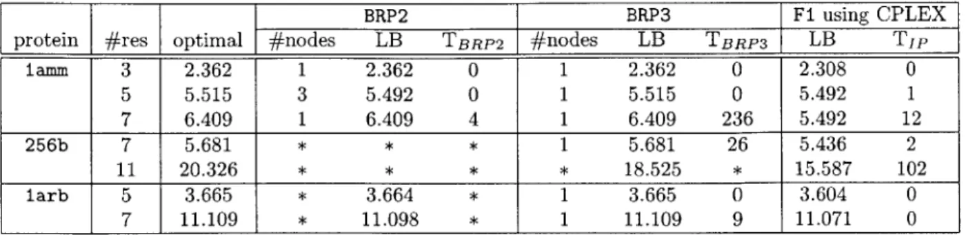
value slows down as the the column generation progresses, often resulting in as many iterations to prove optimality as needed to come across the optimal value. There are techniques to deal with the tailing-off effect such as early termination with the guarantee of the LP-relaxation lower bound [39], but we did not go into them. Table 2.3 and Table 2.4 list the results from BRP2 and BRP3, respectively. Com-paring the results from BRP2 with those from BRP1, BRP2 obviously performs better than BRP1. This seems to be mainly due to the efficient column generation using k shortest paths algorithm and the smaller size of S*. It is interesting that BRP1 man-ages to work comparably with BRP2 for small cases considering |S 1 is huge even for

the small cases. Note that some cases that could not be solved within two hours by BRP1 were solved by BRP2. Looking at the results from BRP2 and BRP3, BRP2 shows slightly better performance in CPU time and the number of generated columns for the cases solved by both BRP2 and BRP3, but BRP3 was able to find optimal solutions for some cases BRP2 failed to do so within two hours. We suspect the size of S* is the main factor in determining the rate of convergence rather than the column generation method.

Since the base formulation has the smallest S*, its convergence will be faster than any other price formulation, yet the purpose of adopting the branch-and-price algorithm is obtaining integral solutions more efficiently by using a tighter LP-relaxation. Unfortunately, we could not validate the concept by testing the branch-and-price implementations on protein energy examples. Instead, we performed a few additional tests of BRP2 and BRP3 with artificial energy examples whose number of

Table 2.2: Test results for BRP1 (IS*I: total number of feasible columns, #nodes: number of explored branch-and-bound nodes, #LP: number of solved LPs until con-vergence, #cols: number of added columns until concon-vergence, (frac): #cols to IS*I ratio, #LPOP: number of solved LPs until reaching the optimal value, #colsop: num-ber of added columns until reaching the optimal value, TLP: time taken for solving LPs in seconds, T,b: time taken for solving subproblems in seconds, symbol - : IS*I

calculation overflow, symbol * : stopped while running).

protein #res

[

S*I I #nodes I #LP #cols (frac) #LPOp I #colsop TLP

[

Tsub

lamm 3 2.6x104 1 2 5 (0.02%) 1 4 0 0 5 - 1 1 7(0.00%) 1 7 0 0 7 - 1 1403 1423 (0.00%) 1381 1401 0 0 11 - 1 228 240 (0.00%) 1 13 1 1 13 - * * * * * * * lbpi 3 5.7x105 1 1 6 (0.00%) 1 6 0 0 5 - 1 1 4 (0.00%) 1 4 0 0 7 - 1 20 25 (0.00%) 1 6 0 0 11 - 1 220 225 (0.00%) 1 6 1 2 13 - * * * 1 20 * * 256B 3 576 1 1 6 (1.04%) 1 6 0 0 5 1.7x106 1 4 10 (0.00%) 1 7 0 0 7 - * * * * * * * larb 3 64 1 1 5 (7.81%) 1 5 0 0 5 - 1 27 38 (0.00%) 1 12 0 0 7 - 1 1 15 (0.00%) 1 15 0 0 11 - * * * * * * * 2end 3 - 1 1 4 (0.00%) 1 4 0 0 5 - * * * 1 11 * * lilq 7 - 1 1603 1608(0.00%) 1 6 33 2 11 - * * * 1 13 * *