HAL Id: hal-01885324
https://hal.archives-ouvertes.fr/hal-01885324
Submitted on 1 Oct 2018
HAL is a multi-disciplinary open access
archive for the deposit and dissemination of
sci-entific research documents, whether they are
pub-lished or not. The documents may come from
teaching and research institutions in France or
L’archive ouverte pluridisciplinaire HAL, est
destinée au dépôt et à la diffusion de documents
scientifiques de niveau recherche, publiés ou non,
émanant des établissements d’enseignement et de
recherche français ou étrangers, des laboratoires
Analogue Audio Disc Records
Jean-Hugues Chenot, Louis Laborelli, Jean-Étienne Noiré
To cite this version:
Jean-Hugues Chenot, Louis Laborelli, Jean-Étienne Noiré. Saphir: Optical Playback of Damaged and
Delaminated Analogue Audio Disc Records. Journal on Computing and Cultural Heritage, Association
for Computing Machinery, 2018, 11 (3), pp.14.1-29. �10.1145/3183505�. �hal-01885324�
Audio Disc Records
JEAN-HUGUES CHENOT, LOUIS LABORELLI, JEAN-ÉTIENNE NOIRÉ,
Institut National de l’Audiovisuel, FranceThe goal of optical playback of analogue audio discs records has been pursued since at least 1929. Several different approaches have been demonstrated to work. But in most cases the playback quality is worse than using mechanical playback. The Saphir process uses a specifically designed colour illuminator that exploits the reflective properties of the disc material to highlight subtle changes in orientation of the groove walls, even at highest frequencies (20kHz). A standard colour camera is used to collect rings of pictures from the disc. Audio signal is extracted from the collected pictures automatically, under user control. When colour signal is not useable, track slope can be used as an alternative. The process is slow — several hours per disc — but has a wide range of operation on recorded and printed discs, from earliest Berliner recordings to recent vinyl records, and its strength is at decoding direct-recording lacquer discs. An Elementary Shortest Path Solver with a reward (negative cost) on the number of turns is used to re-connect all the sub-tracks obtained, allowing to reconstruct, with limited human intervention, the correct playback order. We describe the approach and present the main advantages and drawbacks. The process was used to play back a number of extremely damaged (broken, de-laminated...), physically unplayable records.
CCS Concepts: • Applied computing → Sound and music computing; Hardware → Sensor devices and
platforms; Hardware → Electro-mechanical devices
Additional KeyWords and Phrases: Analogue audio disc playback, Damaged audio disc signal recovery, Audio records scanning, Analogue artefact capture, Representation and manipulation, ICT assistance in monitoring and restoration, Intelligent tools for digital reconstruction, Optical measurement, Rheinberg illumination
ACM Reference format:
Jean-Hugues Chenot, Louis Laborelli, and Jean-Étienne Noiré. 2018. Saphir: Optical Playback of Damaged and Delaminated Analogue Audio Disc Records. ACM J. Comput. Cult. Herit. 11, 3, Article 14 (August 2018), 29 pages.
http://dx.doi.org/10.1145/3183505
1 INTRODUCTION
1.1 Introduction to Analogue Audio Disc Recordings
The first analogue audio discs were recorded as early as 1887, and distributed as commercial products by Emile Berliner in 1890 [65]. Analogue disc records were the main vector for commercial distribution of audio recordings for a century, before being challenged by the apparition of the Compact Disc in 1982. Millions of
This work was supported by European Commission in the framework of PrestoSpace project (FP6-IST-507336 2004-2008), and by French Fonds national pour la Société Numérique (FSN), Cristal project (FSN-AAP1-012085-405850, 2011-2012).
Author’s addresses: J.-H. Chenot, L. Laborelli, J.-E. Noiré, Institut National de l’Audiovisuel, 94360 Bry-sur-Marne, France; email: {jhchenot, llaborelli, jenoire}@ina.fr.
Permission to make digital or hard copies of all or part of this work for personal or classroom use is granted without fee provided that copies are not made or distributed for profit or commercial advantage and that copies bear this notice and the full citation on the first page. Copyrights for components of this work owned by others than ACM must be honored. Abstracting with credit is permitted. To copy otherwise, or republish, to post on servers or to redistribute to lists, requires prior specific permission and/or a fee. Request permissions from permissions@acm.org.
© 2018 ACM. This is the author’s version of the work. It is posted here by permission of ACM for your personal use. Not for redistribution. The definitive version was published in ACM J. Comput. Cult. Herit., Vol. 11, No. 3, 1556-4673/2018/08/ART14 $15.00 http://dx.doi.org/10.1145/3183505
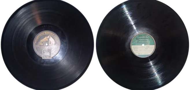
Fig. 1. Left: a printed “shellac” disc (~1920); right: a one-off lacquer “direct recording” disc (1951)
analogue discs have been recorded, billions were sold. Commercially distributed discs were usually printed in multiple samples but it is less known that many discs were actually produced as a unique sample (Figure 1, right). Such unique samples were usually direct-recordings, where a recorded track would be playable immediately after engraving. The main users for such recordings were radio broadcasters but transcription discs were also in use for recording the minutes of meetings, trials, and other events of historical importance. Wealthy amateurs could record their family events. All those recordings participate to the cultural heritage of the 20th Century, and a large fraction, representing millions of records, is critically endangered [8, 14].
1.2 Analogue Audio Disc Recordings Technology
The technique of analogue audio disc recording has been quite stable over more than a century: a horizontal disc rotating at a (usually constant) speed is engraved using a cutter (the cutter is sometimes replaced by a hard stylus that marks the disc surface) [20]. The cutter distance to the disc center is the sum of two components: (a) a slow drift, usually from rim to center, that makes the groove a spiral, and (b) a higher-frequency component depending on the audio signal to be recorded. As a first approximation, it can be considered that the velocity (speed of (b)) corresponds to the audio signal. More complex pre-emphasis filters were often involved, in the view of limiting the radial amplitude, so that consecutive turns would not overlap, and of improving the surface-to-noise ratio (SNR) at higher frequencies. The inverse filters are applied during decoding.
The velocity mentioned above may be radial, as in most mono recordings, or vertical, as in the early sapphire Pathé or diamond Edison hill-and-dale recordings, but also in the case of stereo recordings. In stereo, the radial velocity contains the central signal (Left + Right), while the vertical velocity is used to encode the signal difference (Left − Right). The distance between successive turns of the groove varies between 0.3mm (78rpm discs) and 0.1mm (33rpm long play (LP) vinyl) [59].
The disc may be composed of a whole range of materials including hard rubber, wax, aluminium, vinyl, or a mix of materials known as shellac. Discs may be monolithic, laminated, or coated: laminated and coated discs core material may be cardboard, zinc, aluminium, or glass. Coating may be shellac or cellulose nitrate, blended with filler and plasticisers [4, 13, 50].
Discs may be mass-produced (printed discs) or one-off recorded. Printing is achieved by using the first recording as a mould that is used to make a series of other moulds that are eventually used for pressing the discs by numbers. The one-off recordings case is interesting to us, as such discs — known as instantaneous recordings or lacquer discs — are usually unique examples of the recording, and are much more fragile than printed discs [4]. This makes playing back those unique records a more challenging task than playing back a mass-printed disc. A much more detailed overview by Stotzer of the different disc geometries and materials is available in Reference [59].
1.3 Cracked Lacquer Discs and Broken Discs
Lacquer discs, such as the one on the right-hand side of Figure 1, are actually much more fragile than vinyls or even than older shellac records. This is due to the contrast between the high stability of the core ( aluminium, zinc, or glass…), and the chemically evolving composition of the lacquer that is used as the recording layer. The lacquer contains plasticisers that evaporate or migrate to the surface with time. The layer often tends to shrink and break along fragility lines; cracks appear, in a typical radial/tangential pattern. Zinc-based and glass-based lacquer discs are specifically prone to de-lamination. The whole disc can also break, especially in the case of glass base lacquer discs. Cracked, delaminated, and broken discs cannot be played mechanically, and are challenging to all optical playback processes.
1.4 Why Optical Playback is Tempting
The principles of analogue audio disc recording involve a cutter blade that gouges or imprints a track into a disc. Playing back a disc requires exploiting the physical shape of the disc, to reconstruct as precisely as possible the trajectory of the cutter. This can be done physically, using a stylus to follow accurately this trajectory, but a number of factors make the physical reproduction process less-than-perfect:
Guidance is obtained by physical contact with friction, which inevitably damages the stylus and the recording.
The guidance process should not generate audible oscillations; this is usually achieved by ensuring a dissipative resonance around some low frequency.
The shape of the stylus has to be resistant to friction; it is usually rounder than the sharp shape of the cutter edge; this difference in shape generates distortion.
Any obstruction (e.g., dust) results in a fast motion of the stylus that causes a spike (click) in the output signal, followed by a number of oscillations due to the elasticity/damping in the transmission chain.
The best stylus for one record depends on the groove shape and wear. Testing different styluses is necessary to obtain the best signal.
Nearly since the beginning of analogue audio recording, optical techniques for audio signal extraction from analogue audio disc records have been imagined. Brock-Nannestad ran a thorough research [7] on the patents and inventions as early as 1929, related to using optical processes for recovering audio signal from discs. The author pointedly mentions that the processes based on a direct reading of the recording cutter velocity have a clear advantage in terms of signal quality over the systems that measure the position. It is also highlighted that, for obvious reasons, using light rather than a stylus for extracting the audio signal from a disc recording is less susceptible of damaging the recording medium or the playback device.
As a summary, potential advantages of using optical processes include:
No wear of disc or stylus
Direct detection of dust and scratches, with potential for automated local correction
Ability for playing very damaged records that would not stand physical contact
Ability for playing matrices and stampers
This latest advantage — better signal quality — is, at least by our own experience, only obtained in very rare cases. In our comparisons, the conventional mechanical stylus playback, when possible at all, usually delivers a better quality. But the ability to play damaged records is an advantage that compensates largely for this potential quality loss.
From the processes listed by Brock-Nannestad [7], only the ELP system seems to have worked in practice. It is still sold as a commercial product.
Since then, a number of other approaches have emerged, using 2D or 3D digitization of the record as input data for signal processing and audio signal extraction. They are detailed in the following sections.
2 PRIOR ART ON OPTICAL ANALOGUE DISC PLAYBACK
The optical approaches known to us for optically recovering the audio contents from a disc recording can be classified in three main categories:
Exploiting the reflective/scattering properties of the groove walls to infer the orientation of the groove walls: referred to below as A-Reflective method
Tracking the position of the groove walls using imaging tools: referred to below as B-Imaging method
Using interferometry to measure the distance to the grove walls: referred to below as C-Interferometry method
The following sections will summarise briefly the most significant full-optical approaches up to the present; most references were initially mentioned by Brock-Nannestad [7] or Hamp [26].
2.1 The Finial/ELP Process
The first full-optical process for playing back analogue audio recordings that has met some success was first described in the Stoddard patent, 1989 [57], and was initially known as the Finial process, then as the ELP process. ELP stands for Edison Laser Player. ELP was later renamed as ELPJ, after acquisition by a Japanese company in 1989 [17]. The ELP process works by casting several laser rays at the groove and by using the reflected rays to track the groove and measure the orientation of the groove walls. The orientation is measured using analogue Position-Sensitive-Devices (PSDs) that measure the position of the light spots reflected by the groove wall. All this process is fully analogue. The ELP process is reported to deliver a very high-fidelity playback on vinyl discs in pristine condition. It is also reported to be highly sensitive to disc damage (clicks and pops) [30], and to fail completely on coloured vinyl, shellac, and lacquer discs [23].
Despite those limitations, the ELP system is still sold as a commercial product [16, 17], with a success that was somewhat attenuated by the simultaneous emergence of Compact Disc (CD) [41], but is again boosted by the recent vinyl come-back. The number of units sold is reported to be by the thousands.
2.2 The VisualAudio Process
The Visual Audio process [11, 58] was designed as collaboration between Département d’Informatique de l’Université de Fribourg and Ecole d’Ingénieurs et d’Architectes de Fribourg. It consists of three steps: (1) Preparing a negative real-size photograph of the surface of a disc onto film, (2) Digitizing the negative film at high resolution. (3) Locating and tracking the grooves, and extracting the radial track position as a function of angle. It allows digitizing even damaged discs. The signal quality is fair but suffers from lighting and pictures being taken from top (at 90° angle): more information is available from the disc surface and groove bottom than from the groove walls themselves. The signal is extracted by tracking the positions of top-to-wall and wall-to-bottom transitions. This amounts to at most four tracks, and the result is aggregated into a single audio track. The Signal-to-Noise Ratio (SNR) is fair in the low frequencies but degrades at higher frequencies, since the requirements in terms of resolution increase with the frequency. Considerable work was dedicated
to improving the resolution, including fine-grained film, a large chamber setup, blue lighting, and small optical aperture. Several units are installed, principally in Switzerland. The VisualAudio team achieved a première in 2008 by successfully decoding a number of cracked audio lacquer disc recordings [34], using software tools with operator involvement.
2.3 The Irene Process
The Irene process results from the collaboration of Physics Division of Lawrence Berkeley National Laboratory, the Library of Congress, and the North-East Document Conservation Center, under the impulsion of Carl Haber [18, 47]. The approach is to use high-precision optical measurement devices (confocal probes) to make a 3D model of the disc surface, and to use this 3D model to reconstruct the signal recorded on the disc. Scanning a whole disc using confocal probes is more suited to vertical modulation discs, therefore an “Irene 2D” version was also developed, a scanner that scans the disc surface, obtaining a high-resolution reflectivity picture of the whole disc. This image is then analysed to extract the signal, at this point the process becomes very similar to VisualAudio. The Irene 2D process suffers similar limitations as the VisualAudio process in terms of reproduction of high frequencies. A number of units are installed, principally in the USA (LoC, NEDCC, …). The Irene team has reported success in digitizing at least one broken glass-based lacquer disc [32] and part of one delaminated lacquer disc [33].
2.4 The Flatbed Scanner Processes
A number of independent initiatives have been tried to exploit flatbed scanners to extract the audio signal from the high-resolution images obtained when scanning a record on a flatbed scanner. Most of those works were developed as students training projects up to the early software prototype stage, and are described in web pages or reports such as Springer [55], McCann [44], Olsson [48], Kalla [36]. Feaster [19] actually exploits scans of discs printed on paper as early as 1889.
The main limitation of the flatbed scanning approach is due to the resolution: even at the highest resolution available to those projects (2400 dpi), the minute details required to get a decent SNR at frequencies beyond 5kHz cannot be captured using a flatbed scanner (typical sizes are detailed in Figure 7). Even using the maximum available hardware resolution, at 3600 dpi, pixel size is still 7m. In addition, the Cartesian scanning order and lateral lighting source are also susceptible of generating periodic signal distortion depending on the angle between the scan line and the general groove direction.
2.5 Other Optical Approaches
Although it would be difficult to list all the different tried approaches for reading analogue audio discs using optical tools, the following ones present some interesting features. They are briefly described below.
Juraj Poliak [51] has designed a mixed physical/optical process for analogue audio disc playback. It involves physically tracking the bottom of the groove using the tip of a glass fiber, and extracting the tip position using a lens and a 2D PSD (Position-Sensitive Device). A prototype was built, that runs real-time on discs and cylinders. The glass fiber tip does touch the record but the stress on the groove walls is much lower than using a conventional pickup stylus. Juraj Poliak’s page mentions recovery of one cracked lacquer disc.
Heine [28, 29] uses laser illumination, and wedge-shaped optical fibers bundles to detect the position of the the side lobes of the pattern diffracted by the groove walls.
Hensman [30] uses 2D medium-resolution (~20m) microscopic imaging, lateral lighting, image stitching, and a signal processing chain that appears (after stitching) as very similar to Irene 2D and VisualAudio decoding schemes.
Tian [61] also uses 2D microscopic imaging and lateral lighting, but at a much finer resolution (1m), and generates a 3D model of the groove by computing optical flow between successive images.
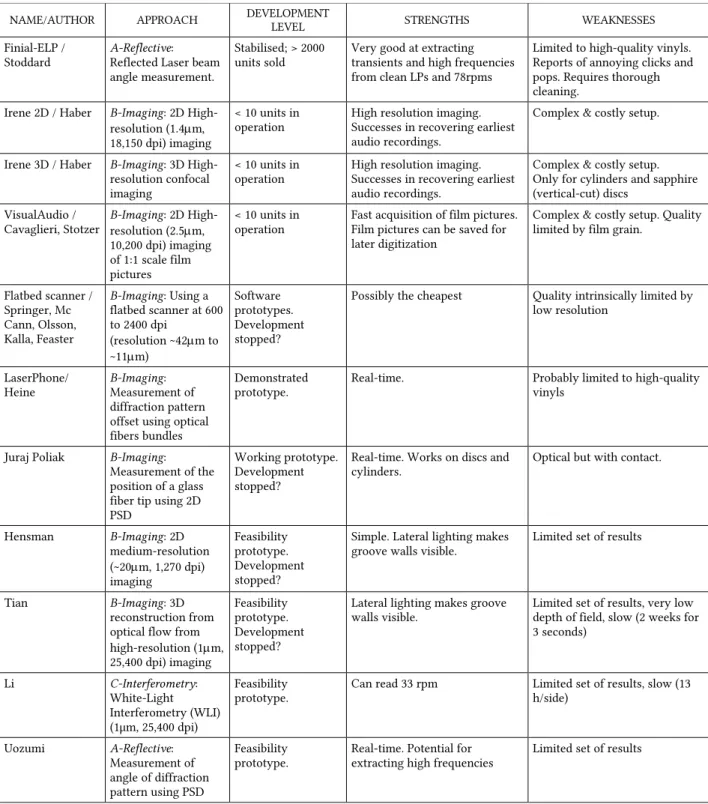
Table 1. The different approaches for playing optically analogue audio disc records
NAME/AUTHOR APPROACH DEVELOPMENT LEVEL STRENGTHS WEAKNESSES
Finial-ELP /
Stoddard A-Reflective: Reflected Laser beam angle measurement.
Stabilised; > 2000
units sold Very good at extracting transients and high frequencies from clean LPs and 78rpms
Limited to high-quality vinyls. Reports of annoying clicks and pops. Requires thorough cleaning.
Irene 2D / Haber B-Imaging: 2D
High-resolution (1.4m, 18,150 dpi) imaging
< 10 units in
operation High resolution imaging. Successes in recovering earliest audio recordings.
Complex & costly setup.
Irene 3D / Haber B-Imaging: 3D
High-resolution confocal imaging
< 10 units in
operation High resolution imaging. Successes in recovering earliest audio recordings.
Complex & costly setup. Only for cylinders and sapphire (vertical-cut) discs
VisualAudio /
Cavaglieri, Stotzer B-Imaging: 2D High-resolution (2.5m, 10,200 dpi) imaging of 1:1 scale film pictures
< 10 units in
operation Fast acquisition of film pictures. Film pictures can be saved for later digitization
Complex & costly setup. Quality limited by film grain.
Flatbed scanner / Springer, Mc Cann, Olsson, Kalla, Feaster B-Imaging: Using a flatbed scanner at 600 to 2400 dpi (resolution ~42m to ~11m) Software prototypes. Development stopped?
Possibly the cheapest Quality intrinsically limited by low resolution
LaserPhone/
Heine B-Imaging: Measurement of diffraction pattern offset using optical fibers bundles
Demonstrated
prototype. Real-time. Probably limited to high-quality vinyls
Juraj Poliak B-Imaging:
Measurement of the position of a glass fiber tip using 2D PSD
Working prototype. Development stopped?
Real-time. Works on discs and
cylinders. Optical but with contact.
Hensman B-Imaging: 2D medium-resolution (~20m, 1,270 dpi) imaging Feasibility prototype. Development stopped?
Simple. Lateral lighting makes
groove walls visible. Limited set of results
Tian B-Imaging: 3D
reconstruction from optical flow from high-resolution (1m, 25,400 dpi) imaging Feasibility prototype. Development stopped?
Lateral lighting makes groove
walls visible. Limited set of results, very low depth of field, slow (2 weeks for 3 seconds) Li C-Interferometry: White-Light Interferometry (WLI) (1μm, 25,400 dpi) Feasibility
prototype. Can read 33 rpm Limited set of results, slow (13 h/side)
Uozumi A-Reflective:
Measurement of angle of diffraction pattern using PSD
Feasibility
Li [42] uses White-Light Interferometry (WLI) to obtain a 3D reconstruction of a 33rpm disc surface. The 3D map is then used for recovering the audio signal in stereo. The decoding process becomes then very similar to the Irene 3D concept. It is stated in Reference [42] that it takes 27 min to scan 1 second of audio on a 33rpm audio disc. This would require more than 13 hours for a standard 33rpm disc side, but it is not mentioned whether such a duration was ever tested.
Uozumi [63] uses a laser as an illuminator, 2D PSDs to measure the general direction of the side lobes of the pattern diffracted by the groove walls, and photodiodes to track the groove. This process bears similarities with the ELP process, using the A-Reflective method, and has the potential of extracting high frequencies.
The work described here only focuses on disc recordings. For completeness, we will also mention two attempts at recovering optically signal from cylinders recordings: the Syracuse Radius project [49], which attempted to use interferometry to read velocity (C-Interferometry method), and the A-Reflective approach by Nakamura et al. [46], related to Uozumi [63], which uses PSDs to measure the position of the reflected spot.
Our process will be detailed in the following sections. We take advantage of the A-Reflective class of methods in terms of high frequencies but, unlike ELP and Uozumi, we do not track the groove directly but exploit 2D imaging for acquiring pictures that are decoded at a later stage, and we can recover the signals from extremely damaged discs.
3 OUR APPROACH TO ANALOGUE AUDIO DISC OPTICAL DIGITIZATION
3.1 The Colour Decoding Scheme
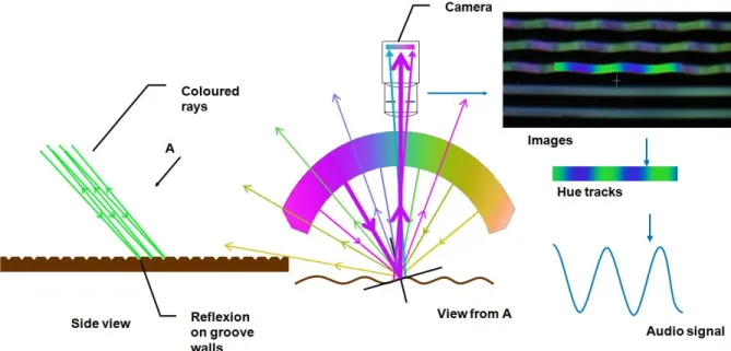
Our initial – and preferred – approach, initially described in References [37, 39, 40], belongs to the A-Reflective method class. It leverages upon the assumption that the groove walls of a lateral-cut disc record behave as a mirror. This is also the assumption that is successfully exploited by the ELP process [56, 57]. Beforehand, this finding has long been exploited for measuring the maximum level of recording, by casting a parallel beam of light at 45° onto the disc surface and measuring the width of the reflected light pattern; this method is known as the Buchmann-Meyer [9, 10] method, illustrated in Figure 2. Using the reflective properties of the groove walls allows measuring the groove wall angle without the need for high-resolution 2D or 3D data.
Our process uses a reflective variation of Rheinberg illumination [53], by casting, onto a small area (2×3mm2) of the disc surface, a wide (140°×15°) light beam from a condenser, where the colour of the rays continuously depends on the illumination angle, as detailed in the next section. The groove walls reflect those colours according to the law of reflection (reflection and incident angles are equal). As a consequence, from a remote viewpoint, the groove walls appear as coloured, and the colour is a function of the groove wall orientation, as shown in Figure 3.
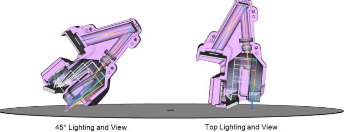
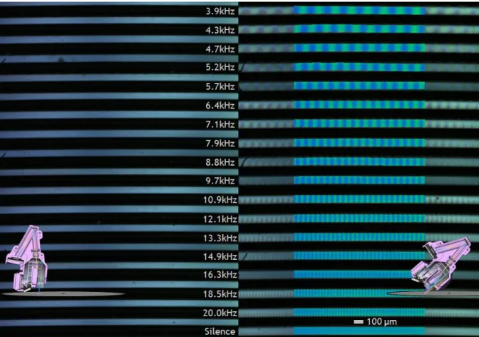
The interest of this principle is that simple colour cameras and optics can be used, contributing to making the scanner affordable, and still performing at high audio frequencies (10 to 20 kHz). This last point is true when the scanning head is in the 45° configuration, shown on the left-hand side of Figure 4. In the top configuration, the colour patterns disappear completely. Figure 5 gives an overview of the differences between 45° and top configurations. In the more detailed Figure 6, the 20kHz signal is still plainly visible, despite the peak-to-peak radial amplitude being already well below our pixel resolution.
Figures 5 and 6 were extracted from the AES Coarse Groove reference disc [3] side visible on the left-hand side of Figure 2, containing a number of useful reference tracks. We are interested here in the inner 20Hz-20kHz sweep track, which is preceded by a 1000Hz tone (−9dB, 7mm Light Band Width (LBW)), and followed by a nominal level 1000Hz tone (8cm/s peak, 20mm LBW).
On this reference disc, the inner 20kHz track is at 75mm from disc center. Tangent speed is 2×75×(78/60) = 612.6mm/s. One full wave at 20kHz spans tangentially over 31m (7.5 pixels). In terms of radial excursion, at 20kHz, LBW = 7mm, which is equivalent to 28mm/s peak-to-peak, or 28/20,000/ ~= 0.45m peak-to-peak radial deviation, as shown in Figure 7. This is below 1/8 of the pixel resolution of our lens+camera setup
Fig. 2. The Buchmann-Meyer method was an easy way of measuring the peak radial cutter velocity, by measuring the width of the reflected pattern from a collimated light source, up to the point the maximum velocity was often expressed in mm Light Band Width (LBW). Left and center: AES coarse-groove 2007; right: a direct-cut lacquer recording.
Fig. 4. The two different configurations for the scanning device: Left: standard 45° degrees lighting and view; Right: top (vertical) lighting and view, only used for comparisons and for discs with a high level of exudates.
Fig. 5. A low-resolution composite view of 3×20 pictures from AES 78rpm coarse groove 2007 test disc track shown on the left-hand side of Figure 2. (a) scanned from top: tracks are dark; (b) scanned at 45°: tracks are coloured; (c) scanned at 45°, after tracks extraction and normalisation of saturation and luminance.
(4m) but the A-Reflective method still allows recovering from colour the 20kHz signal without any sub-pixel processing.
The limiting factor is here the lens+camera tangential resolution (6,350 dpi, 4m on green channel but the colour resolution on blue channel is coarser and closer to the 8m Bayer pattern period).
3.2 Physical Implementation of the Scanner
Our disc scanning process consists in acquiring a relatively large number of overlapping pictures, each covering a 2.6×2mm area. This allows to interactively set up for scanning by examining the current image, and adjusting until it looks good. Colour line sensors (1D) could have been used instead but a more expensive setup would have been necessary, and interactive adjustments would have become trickier.
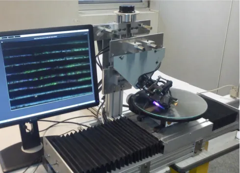
Figure 8 features a view of the system during the scanning of a lacquer disc. The acquisition head position can be adjusted in height and angle. The turntable lies on a translation bench, allowing the acquisition of successive rings of pictures. The disc is kept flat under a glass pane; at 45°, the effects of potential multiple reflections are negligible. On the left, a view of the picture being scanned is displayed.
The scanning head is detailed in Figures 9 and 10. It is designed for ingesting pictures that can be decoded using the A-Reflective method class, as detailed in Section 3.1, but it also allows reading the signal according to the B-Imaging method, when A-Reflective is not applicable, as later detailed in Section 3.3.
On an average 78 rpm disc, we collect, in 3 hours, 60 rings of 1,125 overlapping 640×480 8-bit raw Bayer pictures, which amount to 21Gbytes of storage. The set of collected pictures can be considered as
Fig. 6. A composite of 2×5 pictures from AES 78rpm coarse groove 2007 test disc shown in Figure 2, inner and densest sweep track; signal is accessible on the whole height span of the groove wall, up to 20kHz. Left: viewed from top, tracks are dark and highest frequencies are indistinguishable from silence. Right: scanned at 45° degrees; tracks are blue-green. For a better visibility, saturation and luminance are normalised in the exploited central area.
Fig. 7. An up-to scale top view diagram of a few waves of the 7mm LBW (−9dB) 1kHz, 3kHz, 10kHz, and 20kHz regions of the same track. From 1 to 20kHz, the recording frequency response is flat. Despite peak-to-peak excursion evolves proportionally to the inverse of frequency (from 9m to 0.45m), the peak slopes (excursion×/wavelength) actually increase by 10%, proportionally to the inverse of distance to center.
Fig. 8. The prototype scanning a lacquer record through a glass pane
sub-pictures of a large picture that would cover the whole disc. In that sense, our approach has similarities with several B-Imaging processes mentioned in Section 2. The principal difference lies in the colour decoding scheme detailed above.
All components of the scanner head are either off-the-shelf or 3D printed, with two exceptions:
The coloured filter is printed on a Kodak DS 8650PS film printer.
The 1:1 140°×15° light condenser consists of two total internal reflection optical sector blocks lathe-turned from PMMA (a.k.a. Acrylite™, Altuglas™, Plexiglas™...) and polished.
The light source is an Ostar 1000 Lumen LE-UW-E3B LED, delivering six flashes per second. Two mirrors are used for keeping the scanner head compact. The second mirror is also used for initial frame and focus adjustment. The camera sensor is tilted with respect to the optical axis as per Scheimpflug principle [54], to compensate partially for the disc surface orientation. Our current setup uses a standard-definition 640×480 PointGrey FireFly MV 1394a camera board, and an optical doublet pair from off-the-shelf lenses with 1:1.5 magnification, with a resulting 4×4m source pixel size, and a 2.6×2mm picture size (5.2mm2).
Due to the use of a 2D sensor with medium resolution and electronic shutter, the requirement for stability is not such that an optical bench would be necessary. The current setup is still relatively bulky, due to the whole turntable lying on a translation stage, but we are working on a turntable-sized setup where only the optical head will be translated on a rail.
3.3 The Alternative Slope Tracking Decoding Scheme
The reflective approach, however, presents a considerable drawback, which also affects the ELP system: when the reflection on the groove walls is compounded with diffusion, the reflected signal becomes much more difficult to exploit: we have observed that the colour signal saturation can decrease, negatively affecting the Signal-to-Noise Ratio (SNR). Furthermore, lacquer discs quite often exhibit exudates, whitish spots of exuded plasticizer, often palmitic acid [13]. When those spots are scarcely disseminated, it is relatively easy to discard
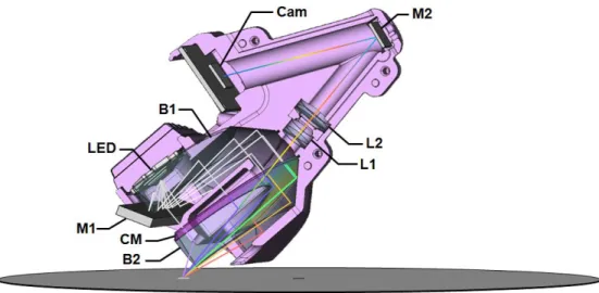
Fig. 9. Partial cut view of the colour scanner head: white light from the 6mm2 LED source is reflected and refracted consecutively by mirror M1, optical sector block B1, coloured mask CM, block B2. Each direction is coded by a different colour. All coloured directions converge towards a 1:1 image of the LED onto the disc surface; rays reflected back along the optical axis are focused through lenses L1, L2, and reflected by mirror M2 onto the colour camera sensor Cam.
Fig. 10. The coloured mask CM. Changes in the central region are steeper, to obtain a better precision at low levels. This is compensated for at the decoding stage.
the information collected in this area by ignoring low-saturation pixels [38], but we also have found numerous examples where the colour information becomes completely unusable, and adds little or no value to the luminance information.
However, a side-effect of our setup has proved to be beneficial: given that our lighting beam is cast at a ~45° angle, the groove wall is in full light. This results in the groove walls exhibiting a set of parallel fine lines that are visible in most cases of coarse-groove records, as shown in pictures Figures 11 and 13. We have not found any literature addressing the exact reason why such lines appear but from our experience this pattern is quite frequent. We assume that the groove walls are corrugated, due to one or several of the following:
Disc cutter edges may have been undulated due to machining process
Lacquer curing may have resulted in stratification
Wear from past physical playback
This pattern is made more visible as our condenser vertical angle is relatively narrow (15°), with main axis perpendicular to the general orientation of the groove wall. The pattern is often interrupted but generally quite visible, even in the presence of a high amount of exudates or dust.
This finding led us to try exploiting as much as possible of those ridges to measure the local groove orientation, trading off highest frequencies against robustness. Measuring the groove slope is a process very
Fig. 11.The same area of a stained and damaged lacquer disc record. Left: using vertical lighting and view, the tracks are dark: only edges, scratches, and occlusions are visible. Right: using 45° lighting and view, grove walls are in full light. In addition to the coloured signal, they exhibit a set of parallel fine lines (ridges), which can be used to measure accurately and robustly the track slope.
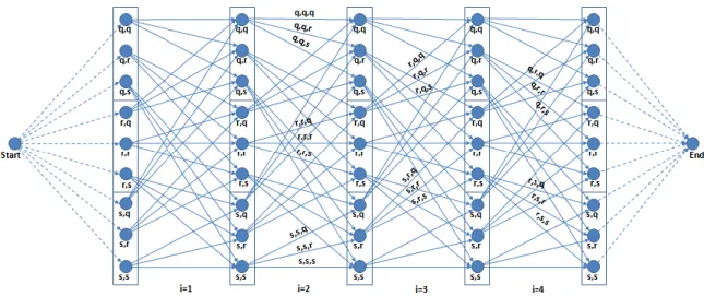
Fig. 12. Each round of the Dynamic Programming approach amounts to finding the shortest path in an acyclic graph, where the cost of each arc is computed by summing the absolute differences between the picture content and the current profile swept along a quadratic spline (arc of parabola) depending on three coefficients. The constraint that the curve is continuous and differentiable is enforced by the structure of the graph, as the second coefficient adjustment of every node is identical to the first coefficient of all nodes it can be connected to. For clarity, the graph is shown for a late round where only three choices (q, r, s) are available as potential adjustments to each coefficient from previous round.
similar to the B-Imaging principles used by VisualAudio, Irene, and flatbed scanner approaches mentioned in Section 1.3, but we have the advantage that our pictures of the groove wall can exhibit two to six parallel ridges.
To build into this process a fair robustness to exudates and other obstructions, we have attempted to obtain, for each track, a spline model, that minimizes the sum, over the track height, of the variations along all paths parallel to the spline. The spline keypoint frequency is set to the Nyquist rate, twice the desired signal cut-off frequency.
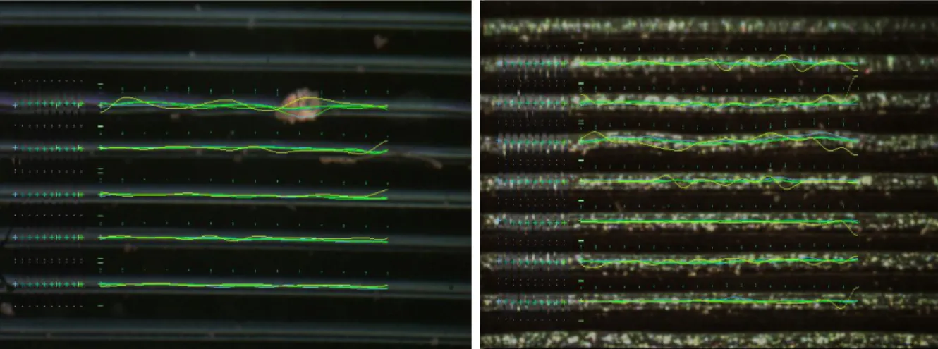
Fig. 13. Images showing how Dynamic Programming can be used to track, with sub-pixel precision, the groove walls position, when the colour signal is not useable. In grey on the left of the pictures are the profiles used for successive dynamic programming iterations. The trajectory colour evolves from blue (first round) to green (final round). The points above the curves show the positions of the spline nodes (set here to 7500 and 10000 points/sec., equivalent to 3.75 and 5kHz cut-off). In yellow is plotted (amplified) the slope of the trajectory, i.e., the recovered signal. Left picture shows that the approach is relatively little disturbed by debris (first tracked row). Right picture shows that a relatively accurate tracking can be achieved, even in the presence of exudates.
To minimise this cost, our first implementation used the Powell COBYLA minimiser [52] from the NLOPT package [35]. This did generate good tracks but made the decoding process extremely slow beyond seven keypoints per track. We then implemented a Dynamic Programming approach that makes the processing time independent of the number of keypoints. The robustness is achieved by alternating between measuring the profile along the current track, and finding the track that minimizes the cost. The new cost is the sum of the weighted absolute differences between (a) the profile translated along the track, and (b) the actual luminance at the corresponding pixels. For robustness, those measured differences are weighted with a weight decreasing with the difference. To guarantee that the slope is continuous, we use standard quadratic B-Splines (three coefficients per spline segment) and only explore the next choice where the 1st and 2nd coefficients are respectively equal to 2nd and 3rd coefficients for the previous choice, as illustrated in Figure 12. This results into a shortest path search in an acyclic graph where the cost of one round is proportional to the cube of the number of distinct coefficient adjustments considered.
The total cost of exploration is limited by allowing nine distinct coefficient values only on the first round, then the number of potential coefficient adjustments is decreased by two at each round until three choices are left (9, 7, 5, 3, 3, 3…). The range of adjustments is also decreased at each round. Thus the first rounds are moderately exhaustive, avoiding as much as possible local minima, and the subsequent rounds allow for a finer, relatively fast convergence, when in the vicinity of the — hopefully global — minimum. The found trajectory is a series of successive arcs of parabola, continuous and tangent at keypoints, but still containing high frequencies due to jumps in second derivative (curvature). Those high frequencies are filtered out using a Gaussian with σ = 0.35 × stepwidth; the output of the decoder is the derivative (slope) of the filtered trajectory.
Our tests have shown a surprisingly robust behaviour, where signals can be extracted nearly optimally from clean tracks with several ridges, still maintaining an output generally free of spurious artefacts or spikes on tracks with occlusions and large amounts of exudates.
Overall, we are in a position where signals can be extracted with full bandwidth from the colour, or with restricted bandwidth using the slope, relying on the ridges still present in the damaged tracks. The subpixel
Fig. 14. Examples of cracked lacquer discs
precision on slope increases with stepwidth and the number of ridges present in the track: if the profile is simple, precision will be better than the two-tracks processes by VisualAudio and Irene-2D. When three ridges are present, which is relatively common, the increase in precision can be roughly estimated to be equivalent to a six-track process, for a result still limited in quality and bandwidth.
3.4 Reconstructing the Path in Simple Cases
In simple cases, the decoding workflow implements the following steps:
Identifying track segments in each picture
Extracting signal from each segment
Joining and blending overlapping segments into groove fragments
Assigning to each groove fragment a playback order
Joining and blending overlapping groove fragments into audio files
Assigning the correct playback order to groove fragments was a more difficult task than anticipated, because, even on a high-quality recent disc, the disc is never perfectly centered, and may be warped, which sometimes results in incorrect ordering when relying for this task solely on the distance to center. To compensate for this, we have modelled a slowly varying radial correction parameter, which is fitted to avoid any ambiguity when deciding on the playback order ranking. This allowed us to output audio files directly from the picture contents. But the workflow described above was far from sufficient to address the cracked lacquer discs problem. The next section is dedicated to this specific issue.
4 ADDRESSING THE CRACKED LACQUER DISCS PROBLEM
As mentioned by Copeland [12] and Pickett [50], lacquer discs add up to a considerable fraction of the production of audio recordings between 1930 and 1960, among others by radio broadcasters, before being replaced by audio tape. Many of these recordings are still not digitized, and a large fraction exhibits cracks as shown in Figure 14, making them impossible to play using a stylus. It is estimated, only within INA, that more than 20,000 such discs are awaiting a solution for recovering the audio signal. VisualAudio and Irene have already demonstrated promising results on those discs [33, 34]. Taking into account the specificities of our tools and of the discs submitted to us, we have developed our own approaches for recovering the signal from such cracked discs.
Fig. 15. Results of the failed Patch approach for adjusting the flakes position. Note that A and B patches have complex shapes, and are distorted in a way that cannot be properly managed by the rigid-shrinkage paradigm. C, D, and E patches should also be subdivided further. This disc could not be completely played using the Patch approach.
4.1 The Patch Approach
Our initial assumption was to consider that the lacquer patches were rigid enough so that, by re-scaling and re-positioning them on the disc map, the geometry would become good enough for decoding the disc using the standard process described in Section 3.4.
After pictures de-coding, we end up with a set of tracks that cover the whole disc surface. We worked on separating this set of tracks into subsets, each subset belonging to a common patch. To be considered as belonging to the same patch, two track fragments had to be close enough to each other, and share a large overlap between their angular ranges. Then we tried to implement a matching method between nearby patches, using track variance as a signature, in a way similar to VisualAudio [34]. But this resulted into a difficult arbitration between obtaining too small or too large patches, as shown in Figure 15. A single patch was often deeply cut into by a crack, and its shape distorted.
Overall, the assumption that the lacquer patches were simply shrunken rigidly proved to be considerably too simplistic for the considered disc samples. This led us to giving up entirely the patch-based modelling, and we have instead concentrated on recovering the best path that would join every single track fragment in the right order.
4.2 The Many-turns Path Approach
We have modelled the best path problem as follows: given a number (up to ~12,000) of track fragments considered as nodes in a graph, and an even larger number of possible jumps (arcs) between those nodes, what is the best possible path from the outer node to the inner node in this graph? The path had to exhibit the following properties:
Fig. 16. Synthetic example. Left: a simplified view of the fragments to be chained. Right: considered successors shown for a few fragments.
From the outer node to the inner node
A simple path: except start and end, every node has either one in and one out selected arcs, or none
Elementary: without subtours (cycles, even with negative cost)
Optimal: avoid long jumps and poor track variance transitions (cost) but use as much as possible of the available nodes (reward, or negative cost)
This kind of problem belongs to the Elementary Shortest Path Problem (ESPP) class. The Elementary term is relevant here because, as we have negative costs (understand: rewards) on a number of arcs, omitting this constraint may result in possible loops with negative costs, that could be run through an arbitrary number of times, making the cost of the path arbitrarily low. When such negative cost loops are possible, the Elementary constraint becomes a condition for the existence of a shortest path. Considerable effort has been dedicated to this class of problems, and it is known that, depending on the constitution of the problem, it can become NP-complete, i.e. extremely difficult (slow) to solve [22].
Starting with simple baseline techniques, we first used the Bellman-Ford [5] algorithm, which is known to deliver quickly the optimal path, provided there is no accessible negative cost cycle in the whole graph (in the presence of such a negative cost cycle, it detects it and stops). Provided that the “reward” was low enough, the Bellman-Ford algorithm did deliver the shortest path, but this path was unsatisfactory, in that it would jump quickly from the rim to the center, avoiding a large subset of the available track fragments, as illustrated on the left-hand side of Figure 17. Increasing the reward would increase the number of turns, but would soon result in the detection of an accessible negative cycle, without any path being delivered any more.
As a consequence, we searched for a more efficient, albeit more computation-intensive, way of solving the shortest-path problem, even in the presence of cycles with negative costs. Haouari [27] presents several ways of solving this problem using mixed-integer programming formulations. In such formulations, the problem can be modelled as minimizing a linear cost function of variables, with constraints expressed as limits on other linear functions of variables. Such variables can be scalar (Linear Programming), integer (Integer Programming), or both (Mixed Integer Programming). Commercial and Open Source solvers for those problems are available.
In our case, there would be as many variables as arcs in the graph; those variables would be binary, as a specific case of integer variables. The value would be 1 if the arc is visited, 0 otherwise. There are a number of formulations, involving a number of auxiliary variables for this problem, as detailed by Taccari [60]. We have first implemented the Miller, Tucker, and Zemlin (MTZ) [45] and Single Flow (SF) [27, 60] formulations, and used the LP-solve solver [6]. We obtained paths that would satisfy the constraints; but the computing cost
Fig. 17. Potential solutions for the synthetic example. Left: an acceptable but too short (low reward) path. Center: without crossing constraints, a high-reward but unacceptable path (self-intersections and cycles). Right: adding the non-crossing constraints makes the problem easier and faster to solve, the best path is found. Note some fragments are dutifully ignored, and a missing fragment is correctly bypassed (bottom-right, fourth turn).
rose considerably, from seconds to hours. Adding additional constraints, e.g., non-crossing constraints or visiting order constraints, increased the computing cost even more. Stopping the computation before the end of the run would result in unsatisfying solutions, with too few turns, or self-crossing paths. It only became clear at this point that the MTZ and SF formulations for enforcing the Elementary constraint were not applicable to our case, as we had too many potential cycles with negative costs.
It is known that the convergence time of solvers on MIP problems is quite variable [43]. The solution may lie in changing the solver but more often in changing the model [1, 62]. We searched for alternative ways of modelling the problem. Drexl [15] states that computing costs for the ESPP can become affordable, under the condition that only binary variables be used, with additional constraints coding for conditions to be avoided. More specifically, Drexl concludes that a fast way of solving the ESPP, is to model the problem using only binary (arc) variables, to obtain a preliminary non-elementary solution that may contain a number of subtours (cycles), to add the corresponding Subtour-Elimination-Constraints (SECs) to the model, and to solve again until an elementary (no subtour) solution is obtained. The fact that potential SECs are “exponentially many” is not too much of a problem, since only the needed SECs are added explicitly to the model. The potential improvement in speed was already promising, but we at this point realized that our model could be adjusted so that very few subtours would be possible in solutions, giving hope for a one-shot solution.
We refined our model to the following formulation, where differences with previous approach are underlined:
From the outer node to the inner node
A simple path: except start and end, every node has either one in and one out selected arcs, or none
Elementary: without subtours (cycles, even with negative cost)
Counterclockwise: considered arcs never go backwards by more than a fraction of a mm
Non-crossing: a selected arc should not cross another selected arc, or a selected node (track fragment)
Optimal: avoid long jumps and poor track variance transitions (cost) but use as much as possible of the available nodes (collecting reward, or negative cost)
The combination of the “Non-Crossing” and “Counterclockwise” constraints satisfies in most cases the
Elementary constraint and makes SECs unnecessary, as illustrated in Figure 17. Allowing subtours makes the
problem easier to formulate and faster to solve. In the infrequent cases where subtours still come out in the solution, they can be safely ignored (cycles of two close very small fragments), or are due to an imprecision in the computation, or omission of non-crossing constraints. They can be corrected interactively as shown in the next section.
Fig. 18. The decoding interface, with all potential arcs displayed in grey
The presence of numerous cliques (mutually-exclusive binary constraints) in the model led us to test and adopt SCIP_solve [2, 21] as a new solver, which did solve our problems much faster than LP-solve.
We are now in a position where solving the complete ESPP for one disc side with a few cracks usually takes less than one minute. In cases where there are numerous track fragments (> 10,000 nodes, potentially > 60,000 arcs) the time increases up to several minutes, or more. But in that case we can stop the solver and run again on a reduced number of rings, and interactively tune the problem to make it faster to solve, as described in the next section.
4.3 A Graphical User Interface for Tuning the Many-Turns Path Approach
In simple cases, directly feeding the ESPP to the solver leads to a satisfying path. But it is often the case that the solver states no solution is achievable, or that the number of turns of the spiral is lower than desired, or that the found path is incorrect, e.g., a large jump is made instead of using a seemingly valid track fragment... The possible origin for such flaws has to lie in the submitted ESPP itself, but the solver does not tell where. We developed specific tools in the graphical user interface shown in Figures 18 and 19 to help the user understanding where the problems lie. Most of the found problems are due to one of the following conditions:
A needed arc is not available as a variable to the solver
The desired path is self-intersecting
A track fragment should be cut across a crack to allow for alternative arcs
A track fragment is missing, and a good arc for bypassing is not available in the model
Insufficient reward for additional turns
Our graphical user interface allows us to examine in detail the ESPP and solution, if any. When unsatisfying, we have the possibility of running the computation again with different parameters, or on a reduced set of rings.
In addition to changing global parameters, it is also possible to act locally, using graphical branching directives such as:
Fig. 19. The decoding interface, highlighting the solved reconstructed path. Note the jumps over missing parts (top left and center views).
Recommended Area: for each node finishing in area, only the arc that matches the area pattern is allowed
Mandatory Area: for each node finishing in area, the arc that matches the pattern has to be used
Shortcut Arc: a new arc can be added to the set of available arcs. This new arc is allowed to cross any arc or node
When the right path is found on a set of rings, it is possible to freeze the section, e.g., by using a number of Recommend/Mandatory Areas; this has the further advantage of reducing, often dramatically, the computing cost on next computation rounds.
The tool is not used to force all connections but rather to constrain the problem so that the solution comes faster and closer to the desired result. Actually, when one adds too many directives, the solver often comes out with no solution at all. Finding out why can be made easier by temporarily adding one or several Cut Areas, as defined later in Section 4.4, to relax the problem, get a solution, and figure out the location of the conflicting constraints.
This tool has allowed us during 2016 to successfully reconstruct more than 20 severely damaged lacquer disc sides. In the worst cases, several patches were missing, and the radial jump between joined tracks was as much as 8 times the distance between tracks.
Table 2 gives typical orders of magnitude in effort and solving times for a number of cracked or broken lacquer disc sides.
The effort in reconstructing a cracked lacquer disc depends on the disc condition. In extreme cases, several hours of work are still necessary. After practising on 10–15 disc sides, we can locate more easily where the problems lie (e.g., a candidate connection missing in the model, or a fragment that should be cut in two), and the effort and number of directives can be reduced: on an average cracked disc, directives generation usually takes less than 20 min.
Table 2. Typical Sizes, Number of Branching and Cut Directives, and Preparation and Solving Times for the Many-turns Approach
4.4 Finding the Cracks
Given the specificities of our lighting and scanning process, cracks can either appear as light or dark, textured or not, without easy identification criteria, unlike as in Reference [34]. Therefore, we have not attempted to locate the cracks from the picture content but rather from the extracted tracks. For each track sample, we have access to a confidence value that is obtained by measuring by how much the track stands out against the dark background. This confidence value is useful not only for locating cracks but also for deciding whether the sample has to be used, or rather repaired, as detailed later in Section 5. By setting a threshold on the confidence level, we are in the position to decide that a span of samples is not useable, because of dust or because of a crack. The track is then cut at the position of the damaged samples.
But it happens that, in the presence of a narrow crack, or of a spurious piece of dust or exudation, a track that crosses a crack is not cut. This is not a problem when the parts of the track on both sides of the crack belong to the same turn; but when they belong to a different turn, it becomes necessary to cut the track where it crosses the crack.
In the case of the Patch approach mentioned in Section 4.1, we detected patches connected by a few tracks, and could cut at the boundaries. In the case of the many-turns approach, there is no notion of a patch, but the graphical user interface was extended to provide for a new directive:
Cut Area: any Track fragment intersecting with area is cut, and new arcs are generated An example of the insertion of such Cut Areas is shown in Figures 20 and 21.
Currently, the user has to draw as many rectangular Cut Areas as necessary. This is time-consuming as, depending on the condition of the disc, a number of such regions may be necessary for one single narrow diagonal crack.
Allowing for more complex shapes should be faster, especially when generated by software processing; we are therefore working on an automated crack detection tool that will, from confidence signals, identify the radial cracks, and will force new cuts where necessary. It is expected to help cleaning up the cracks and to reduce the need for manual interventions.
5 NATIVE DE-CLICKING ON JUMPS, DUST AND SCRATCHES
Even when decoding a clean shiny disc scanned under a glass pane, there are usually places where scratches, or dust pieces, result in a spot in the picture that obscures the underlying signal. Exudates are greasy spots of
DISC SIDE STATE NODES ARCS BRANCHING/CUT DIRECTIVES PREPARATION / SOLVING TIME Cabaret Dolto disc 13, side 25 A few cracks 1484 10336 0 / 0 0 min. / 2 s Fado Mouraria, Maria Teresa de
Noronha, 1939 Aluminium base, many narrow cracks 2638 8337 19 / 43 5 min. / 6 s Poésie en Suède, disc 2, side II Broken glass-base 3504 16704 43 / 61 10 min. / 30 s Dargent, box 73, disc 1, side A
(V) Zinc base, flaking off 2485 7189 351 / 239 2 hours / 6 s
Dargent, box 73, disc 2, side A
(III) Aluminium base, heavily spotted 12570 64164 79 / 110 2 hours / 200-500 s Voici ma carte, disc 2, side 2,
Fig. 20. On this view, a number of branching directives (green boxes) are visible. The reconstructed path is not correct (missed fragment in cyan, subtour in yellow) due to missing cuts on the narrow crack on 3rd, 10th, and 14th turns (white arrows). The long selected arc in orange comes directly from the start fragment, and is not submitted to non-crossing constraints.
plasticiser residue that can affect the signal extraction, sometimes up to the point where the track becomes visible only as a series of aligned bright spots (e.g., Figure 13, right). The confidence channel mentioned in Section 4.4 allows us to store how confident we are that an audio sample actually contains valid signal. Currently the signal only exploits the pixels that are in the acceptable colour subspace. This is far from perfect, but we have confirmed visually that a drop in confidence usually corresponds to a spurious signal peak. Without correction, these peaks are audible as distinct clicks, or crackle if they are frequent. In the case of cracked lacquer discs, at each selected arc, we have to make the connection between the signals from the two connected track fragments (nodes). The signal is usually distorted at both ends of the fragments, and the position of the fragments ends is not known with full accuracy, which results in a few samples missing or in excess. Therefore spurious signal is also present at connections between track fragments.
Of course, good de-clickers already exist, but we have the advantage here of having an estimation, based on the confidence signal, of where the audio signal is reliable, and where it has to be repaired. We have therefore built a tool for reconstructing the missing signal. This tool is fed with an audio signal track, an associated confidence track, and a confidence threshold below which the signal is to be regenerated. Our first version used a Least Square Auto Regressive (LSAR [24, 25]) process implemented in Gnome Wave Cleaner [64]. But LSAR cost is quadratic in terms of the number of samples to be reconstructed, and, when the known good signal data is too scarce, it tends to generate high energy peaks. This led us to design our own tool. The tool works on a large window of signal (up to 16,384 samples), and alternates between (a) spectrum coring in the spectral domain (reducing the spectral components where low), and (b) re-enforcing the known samples to the original value in the temporal domain. After relaxation (always faster than 1 sec), the values of the samples to be repaired are copied back into the audio track. This crude process is similar to Projection onto Convex Sets (POCS) applied by Hirani to missing samples in images [31]. It ensures that the minimal energy signal that goes through the known good samples is recovered. When only a few clicks are corrected, it is usually impossible to tell where the corrections have taken place. But we also have successfully used this process even in cases where a large fraction (> 50% of samples) has to be re-constructed, e.g., for de-clipping signal: at this level of reconstruction, audible artefacts do emerge, but clicks and crackle are still considerably reduced.
6 SIGNAL QUALITY
When mechanical playback is possible, signal quality is usually audibly better than using our optical process. In rare cases, on very shiny discs, we have been able to extract audio tracks that were difficult to audibly distinguish from their mechanical playback counterpart. We have tried to measure the quality of the recovered signal using our process, using as a reference the AES Coarse Groove reference disc [3]. This is one of the rare 78 rpm discs that we could use, as other reference discs available to us are already degraded lacquers. Frequency response is good, as shown in Figure 22. On the inner track, 20kHz is at 75mm from centre. We have on this track a nearly flat frequency response until 5kHz, −6dB at 11kHz, −12dB at 17kHz. On the outer track, the 20kHz is at 127mm from center; sampling frequency is nearly doubled, and frequency response is significantly better (−8dB at 20kHz).
We have also, exploiting the strength of Colour decoding, measured THD+N at 3.1% in the 20Hz–20kHz band on the inner 1kHz reference level (20mm LBW) test signal of the same Coarse-Groove AES test disc, side A [3]. This is not fully satisfying, but we expect to reach a better THD+N after re-calibrating the system.
We have also measured a bit depth of some 11 bits on the same track, by confirming that THD+N stayed at 3.1%, even after applying a −30dB amplification, storing in 16 bits/48kHz, and re-amplifying.
Using the Slope decoding scheme, however, THD+N stays over 18% (−15dB SNR) on the same section; this is in the same range as found by VisualAudio ([59], p179): −19dB SNR on a 78 rpm between 500 and 10,000Hz. We expect to obtain a slightly better result on lacquer records exhibiting the ridges mentioned in Section 3.3 but we do not have access to a lacquer equivalent test record. When the disc presents a high level of exudates,
Fig. 22. The Frequency Response, measured on the AES 2007 Coarse Groove Test Disc, after correction of pre-emphasis (time constants 3180sec / 450sec / 0sec: no effect beyond 1000Hz). The inner sweep sequence exhibits a somewhat poorer frequency response, principally due to the limitations in the optical setup.
the quality is still very poor, and noise often pre-dominates the recovered signal. From those findings, we estimate that in most cases signal quality will be, using our system, poorer than when using a well-calibrated mechanical playback process with the most appropriate stylus. For this reason, we are currently focusing on discs that cannot be played using a stylus: broken/cracked/delaminated records, matrices, oxidized discs.
7 APPLICATIONS
7.1 Advantages of the Process
Being fully optical, our process does present a number of advantages over the mechanical process. It also presents advantages against other optical processes. Among others:
Affordable components
No selection of stylus is necessary; parameters may be adjusted after scanning
No friction on the grooves
Disc can be scanned through a glass pane, that flattens the disc and keeps de-laminating flakes flat and in place
Small obstructions can be read through
Stampers and matrices can be read directly
Disc cleaning is not necessary
Good frequency response: up to 20kHz on 78 rpm discs
Colour and/or Slope signal extraction can be used, depending on the disc surface condition
Reconstruction of severely cracked or broken discs using a Mixed Integer Problem solver for the
7.2 Cases Where our Process is Less Applicable
Our process is currently not applicable to: Stereo recordings: our process only reads one channel; post-synchronisation of two channels was tested but is not finalised
Fully de-laminated discs… but who can read those?
Lacquer discs with transparent coating (Metallophon, discoloured Thorens…)
Coloured vinyl prints
Vertical-cut discs (Pathé, Edison...)
Cylinders recordings
7.3 Success Stories
Starting in 2016, we were able to extract the signal from a number of discs, some of them previously considered as irrecoverable. The first two were a set of two broken glass-base lacquer discs. The 9 and 17 pieces were carefully positioned tightly together, stabilised under a glass pane, and scanned. As the re-positioning of the different pieces was not perfect, a number of cracks were still visible on the scans. These three disc sides justified considerable re-working of the many-turns approach described above in Section 4.2, but we eventually succeeded in recovering the complete set of three sides. The signal quality obtained was surprisingly good, given the initial condition of the records.
We were also able to scan completely several 33rpm metal stampers of unknown origin, dated 1953. After playback, we were able to identify Pierre Schaeffer as the speaker, and then the discs as the original stampers for a limited-edition vinyl case “Dix Ans d’Essais Radiophoniques, du Studio Au Club d’Essai : 1942-1952”.
We then experimented with a number of recordings, most of them without an existing known digital track. For example, we were able to recover the content of lacquer disc cabaret recordings dated 1951, with various levels of de-lamination. We then concentrated on recovering the contents of heavily delaminated zinc lacquer discs. We were able of successfully recover a number of such recordings from 1946 to 1951. This still requires manual work, especially in the presence of cracks and missing parts, but practice and improvements in the process make this process progressively faster.
The Saphir process was used to successfully recover broadcasts in Spanish on the French radio of the Spanish Diaspora community (1946-1950), and the live audio recording in Montmartre (Paris) of the first post-war spade duel in France, between two French painters, recorded on July 5, 1946. The object of the dispute was... Pictural Existentialism !
Recently, we could recover using the same approach the first-ever recording of the fado singer Maria Teresa de Noronha, dated 1939.
The pictures in Figure 23 give an idea of the level of destruction that can be recovered exploiting the Saphir process. Audio track samples of the recovered records above are available at URL
http://recherche.ina.fr/eng/Details-projets/saphir.
8 DISCUSSION
We present here a scanner and decoder process for optical digitization of analogue audio disc records. First, we try to cover pre-existing optical approaches for this task and classify them in three classes. We show that most of the approaches use the B-imaging or the C-Interferometry methods. Saphir uses the A-Reflective method, also exploited by the only system that achieved a commercial success, the ELP system. We give details on how the scanner and the decoder work, and present the advantages of the A-Reflective method in terms of signal quality. We also show how our decoding process can also use the B-Imaging approach when needed. We then explain how we address the difficult problem of reconstructing the signal from broken, cracked, or de-laminated disc records, using a Mixed Integer Problem solver for solving a specific case of the
Fig. 23. Examples of disc, listed in Table 2, successfully digitized using Saphir. In lexicographical order: Poésie en Suède, disc 2, side II; Fado Mouraria, Maria Teresa de Noronha, 1939; Voici ma carte, disc 2, side 2, 1946; Dargent, box 73, disc 1, side A (V).
Elementary Shortest Path Problem. As this process still involves some operator input through the Graphical
User Interface (GUI), we give an estimation of the efforts still needed, and provide leads on how to limit them. We conclude by giving indication on the quality achievable with our system and provide examples of discs in severe condition that could be saved using Saphir. The presented advantages make our process particularly suitable for the recovery of very damaged discs.
9. FUTURE WORK
The work presented here is still in progress. We intend to further work on a number of points. First, the scanner presented here is still a unique sample, and is very slow (3 hours for one disc side). We intend to work on the development of a compacter and faster scanner that can be replicated easily. The footprint of this scanner will be comparable to the one of a standard audio turntable.