A COMPARISON OF SPHERICAL GRIDS FOR NUMERICAL INTEGRATION OF ATMOSPHERIC MODELS
by
DAVID L. WILLIAMSON
B.S. The Pennsylvania State University (1963)
M.A. The Pennsylvania State University (1965)
SUBMITTED IN PARTIAL FULFILLMENT OF THE REQUIREMENTS FOR THE DEGREE OF
DOCTOR OF PHILOSOPHY
at the
MASSACHUSETTS INSTITUTE OF TECHNOLOGY April, 1969
Signature of Author . .,... -... .. ". ..-. ,... Department of Meteorology, April 10, 1969
Certified by . ... Thesis Supervisor
Accepted by ... ... ... ... Chairman, Departmental Committee on Graduate Students
A COMPARISON OF SPHERICAL GRIDS FOR NUMERICAL INTEGRATION OF ATMOSPHERIC MODELS
by
DAVID L. WILLIAMSON
Submitted to the Department of Meteorology on April 10, 1969 in partial fulfillment of the requirement for the degree of Doctor of Philosophy.
ABSTRACT
The properties of spherical grids are reviewed and compared with one another. A quasi-homogeneous spherical geodesic grid is introduced to eliminate many of the undesirable features of other grids. The spherical geodesic grid is first compared with the other grids for integrating the nondivergent barotropic vorticity equation. Initial conditions are used for which an analytic solution exists. The spher-ical geodesic grid produces the best solution. The only observable error in the contoured output is a small phase error.
Methods of developing difference approximations for the primitive barotropic modcl over triangular grids are first considered in cartesian
geometry. Comparative integrations show that the six-point differences assoctated with triangular grids produce better solutions than square differences with similar resolution and the same order of triin-ation error.
Conservative difference schemes are introduced for the primitive barotropic model over the spherical geodesic grid. The small variation
in the grid interval means that conservative schemes which are second order over regular grids are first order over the spherical geodesic grid. This truncation error can be made insignif-icant by taking a fine enough mesh. Comparative integrations indicate that the spherical geo-desic grid produces results that are at least as good as those produced by the schemes currently being used for numerical weather prediction.
Thesis Supervisor: Edward N. Lorenz Title Profesbor of Meteorology
-3-TABLE OF CONTENTS I INTRODUCTION 5 II SPHERICAL GRIDS 7 2.1 Conformal coordinates 7 2.2 Spherical coordinates 11
2.3 Spherical geodesic grid 15
Figures for Chapter II 20
III NONDIVERGENT BAROTROPIC MODEL ON THE SPHERE 25 3.1 Finite Difference Approximations 25
3.2 Initial Conditions 29
3.3 Errors in initial time step 29
3.4 Twelve-day integrations 33
Figures for Chapter III 37
IV PRIMITIVE BAROTROPIC MODEL ON A PLANE 44 4.1 Conservative difference approximations 49
4.2 Individual approximations 53 Pressure Gradient 55 Mass Flux 57 Momentum Flux 59 4.3 Homogeneous grid 59 4.4 Truncat in erro 63
4.6 Boundary conditions 67
4.7 Numerical integrations 69
Figures for Chapter IV 73
V PRIMITIVE BAROTROPIC MODEL ON THE SPHERE 81 5.1 Conservative difference approximations 82
5.2 Numerical experiments 89
Gravity Waves- 90
Neamtan Waves 92
5.3 Initial tendencies 97
5.4 Truncation error 102
Figures for Chapter V 109
VI CONCLUSIONS 122
6.1 Conclusions 122
6.2 Suggestions for further research 126
Acknowledgements 128
Appendices 129
1 Relations used to simplify truncation
error expressions 129
2 Computation of 134
References 136
-5-CHAPTER I
INTRODUCTION
The advent of today's large fast computers has made it practical to experiment with atmospheric models defined over the entire sphere. A spherical domain eliminates the need for artificial side boundaries which introduce spurious results into the regions near them and also makes it possible for general circulation models to study the
inter-actions between the tropics and mid-latitudes as well as between hemispheres.
There are two main methods used today to model the atmosphere over a sphere: expansion into spherical harmonics and discrete approx-imations over grid points. In the first method, or spectral method, all the variables of the governing equations are represented by a series of spherical harmonics. The pr'egnostic equations then become prognostic equations for the amplitude of each spherical harmonic and the evolution of these amplitudes is calculated in time. In the grid point method the variables of the governing equations are replaced by a discrete set of variables defined at a set of grid points over the sphere. The continuous differential operators of the governing equa-tions are replaced by discrete operators defined over the grid points. The evolution of the discrete variables is then calculated in time.
The first spectral integration was carried out by Baer (1964) for the vorticity equation. Ellsaesser (195G) p- rformed comparison
integrations between the grid point and spectral methods for a slightly more general model. He concluded that for these simple models the spectral method produces better results than the grid point method. However, for models based on the complete meteorological equations
the desirability of the spectral method becomes questionable. Robert (1966) performed a successful integration of the complete equations; however, not all the physical processes occurring in the atmosphere were included.
Satisfactory methods of handling phenomena such as precipitation have not been developed for spectral models. Robert (1968) is current-ly studying them. This lack of such methods plus the large number of interaction coefficients necessitated by the desirability of fine reso-lution have led almost all experimenters modeling the general circula-tion to use grid point methods. For this reason, the remainder of this report will deal with grid point methods.
Fundamental problems which naturally arise with grid point methods
are
the definition of the grid points themselves and the development of discrete approximations to be applied at these grid points. Various grid systems over a sphere and accompanying difference schemes have been suggested in the last decade and tried with varying degrees of success. As will be seen in the next chapter, these schemes all have some undesir-able property. One property which few of these schemes possess yet which seems desirable is homogeneity. A new quasi-homogeneous grid is also introduced 4in the next chapter. In the following chapters difference approximations are developed for atmospheric models and evaluation ex-periments are compared with exex-periments using other schemes.
-7-CHAPTER II
SPHERICAL GRIDS
The nets of points suggeoted to date for use with discrete approx-imations fall into three main categories: nets based on conformal map coordinates, nets based on spherical coordinates, and quasi-homogeneous nets independent of the coordinate systems. We consider each category in turn.
2.1 Conformal coordinates
In order to use mappings for numerical studies, the do main of interest, in our case the sphere, is projected onto a section of a plane. A net of points is then defined on the projection. This net can be considered as the projection of a net of points originally on the sphere. Following Kurihara (1965b) we refer to these points on the sphere as the original grid.
Conformal mappings are used in metacrology in order to preserve the general form of the hydrodynamical equations when written in terms of the map coordinates. The difficulties of using conformal mappings for spherical studies arise from the impossibility of mapping the entire sphere conformally onto a finite section of a plane.
The use of a uniform grid on a Mercator projection
is
clearly unsatisfactory for spherical integrations. With such a grid, the original grid interval becomes infinitely small at high latitudes and the pole, at infinity, cannot be reached. Kuo and Nordo (1959) haveused a grid, similar to the one proposed by Richardson (1922), with square meshes of variable size on a Mercator map. Their grid increment was doubled at 60 and again at two higher latitudes. The pole was
represented by an extra row of six points which were close but not at the infinite pole. Kuo and Nordo integrated the quasi-nondivergent model developed by Kuo (1956) over one hemisphere using Green's method. Initial conditions were for mean zonal flow with a somewhat random dis-turbance superimposed. The integration was carried out for six days using a l} hour time step. It was not possible to continue the compu-tations for a longer period because a computational instability
developed after the fifth day. This instability was apparently connected with the change in grid size at 600. The instability plus the inability to properly handle polar phenomena make this type of grid unsuitable for spherical integrations.
Smagorinsky, Manabe, and Holloway (1965) have integrated the primitive equations over one hemisphere using a uniform mesh on a stereographic projection. Such a grid is not homogeneous over the hemisphere. The original grid increment varies by a factor of two from pole to equator. It seems possible to integrate over an entire sphere using two such grids, one for each hemispherical projection. A square mesh on one projection has some points which lie outside the equator on that projection and which have a corresponding position inside the equator of the other projection. Such points do not in general corre-spond to grid points of the other projection and some sort of intevpo-lation scheme is needed to provide values of the variables at these
-9-points. If energy conservative schemes are desired they are very difficult to formulate using these interpolated values. Also, as will be seen in the next paragraph, great care must be taken in the inter-polation formulation to eliminate spurious small scale features from
appearing in the integrations.
In order to obtain a more homogeneous grid, Phillips (1957) proposed using a stereographic map for high latitudes and a Mercator map for low latitudes, connected at middle latitudes by overlapping
grids. With this system, the original grid interval changes by only a factor of 1.4. Phillips (1959) performed a numerical test to check the stability of his system since the scheme was too complicAted to examine theoretically. He integrated the primitive equations for a barotropic atmosphere for a period of two days using Eliassen type finite-differencing. The initial conditions were defined to be a Haurwitz wave of wave number four. Haurwitz (1940) has shown that in a non-divergent barotropic atmosphere, such a wave will move from wiest to east without change of shape with a known constant angular velocity equal to 130 per day for the initial conditions chosen by Phillips. Because of divergence due to the free surface in Phillips' model, the
rate of progression of his flow pattern should be less than that given by Haurwitz.
The wave in the numerical experiment moved about 9 per day, ifi rough agreemenL wiLh whaL was expecLed. The fields remained quite smooth. The isolines agreed well with one another where the two maps overlapped except for two small areas. Two small temporary "wiggles"
appeared during the course of the integrat-ions. They appeared only near the top boundary of the Mercator grid, the stereographic grid values being quite smooth at all times. Phillips concluded that the "wiggles" were some peculiar type of truncation error.
A further study by Phillips (1962) suggested that these trunca-tion errors can be eliminated by changing the finite difference formula-tion. After reformulating the differences he repeated the same baro-tropic forecast as in the first test. The new system did avoid the peculiar truncation errors near the boundaries. This forecast was
continued to three days. The tields were perfectly smooth and resembled the initial data very closely. Phillips1 later carried out a 12 day integration with no trouble.
Even though with careful formulation, difference schemes work over this grid, the basic idea of interpolating between two grids at mid-latitudes where much is happening does not appeal to most investi-gators. Also, the problem of formulating energy conservative schemes
is very difficalt and has not been treated successfully to date.
Because of these difficulties caused by the impossibility of conformally mapping the entire sphere onto a finite section of the plane,
investi-gators turned to grids based on the sphere itself and to polar spherical coordinates.
1
-11-2.2 Spherical coordinates
The immediately obvious grid of this class is one with grid points at intersections of equally spaced latitude and longitude lines.
In this case, as the pole is approached, the meridians converge and the linear distance between grid points in the longitudinal direction approaches zero. This convergence places a severe restriction on the maximum allowable time increment through linear stability conditions. Such a grid is also far from homogeneous.
Most grids in this class have been designed to avoid the small time step required by the convergence of grid points in the polar areas. The atmospheric general circulation models that are presently being integrated over the entire earth all use grids of this kind.
Gates and Riegel (1962) designed a grid, similar to that proposed by Pfeffer (1960), to avoid the small time step. In their grid, the
latitudinal increment was fixed while the longitudinal increment increased by multiples at higher latitudes. The increment was first ircreased at
45 0, then again at 700 75 , 80 , and 85 .
As a first test of their grid system, Gates and Riegel integrated a non-divergent barotropic model for a period of several days. Initial conditions were for a wave that should move with an angular velocity of 20 per day without change of shape. Since the analytic solution for their model is known, numerical errors can be determined exactly. After a ten day period of integration, their solation had a pronounced distor-tion in the form of a backward tilt. This tilt first appeared near the latitude where the longitudinal increment was first doubled. Thus the
phase truncation error is a function of the longitudinal grid increment and increases where the grid interval increases.
This artificial tilt in the wave structure being modeled produces erroneous momentum transports which in turn produce a wrong distribution of the easterlies and westerlies in the solution. Thus general circula-tion models with this type of error produce statistics inconsistent with the original continuous model. This would be a serious flaw in general circulation model approximations.
In an effort to reduce this wave distortion in middle latitudes, Gates and Riegel (1963a) changed the grid so that the longitudinal in-crement first doubled at 750, The numerical test was repeated. The distortion at mid latitudes was eliminated, but the effect of the incre-ment increase at higher latitudes was not considered, there being little happening there.
As additional tests, Gates and Riegel (1963b) integrated the barotropic model, the level quasi-geostrophic model, and the two-layer balanced model of variable static stability. The equations were all formulated in terms of a streamfunction for the non-divergent part of the wind and a potential function for the irrotational part. Initial conditions were atmospheric data for OOGCT, 7 December 1957. No diffi-culties due to the doubling of the grid increment were reported.
A disadvantage of this grid, in addition to the differential phase truncation error, is that the time increment is still limited by the convergence of the longitudinal grid increment up to 70 where the linear grid interval is less than half its value at the equator.
-13-Kurihara (1965b) has defined a grid in which the longitudinal grid increment changes more gradually with increasing latitude. In fact the linear grid increment actually increases with increasing latitude. Kurihara defines N+l equally spaced latitude circles from the pole to the equator. He places 4N grid points around the equator. At each successively higher latitude the number of grid points is decreased by four, resulting in four points next to the pole and one point at the pole.
Kurihara (1965b)carried out successful test computations using a barotropic primitive equation model. However his scheme was quite complicated, involving a number of interpolations. In a later paper
(Kurihara aid Holloway, 1967), he avoided these complications by using difference equations formulated by means of the so-called box method. Integrations with a nine-level model produced seemingly satisfactory results. These results, however, are not useful for comparison with other schemes because of the complexity of the continuous model.
Gary (1968) performed rather extensive comparisons between difference schemes which have been used for general circulation models over Kurihara's grid and over Gates and Riegel's grid. These integra-tions will be considered in more detail in later secintegra-tions for compari-sons of our schemes with those currently being used for numerical experiments. It suffices to state here that he found Kurihara's
Grimmer and Shaw (1967) attempted to eliminate the differential phase truncation error by using a variable time step. In their
scheme, the longitudinal grid increment remains constant and the time step is decreased with increasing latitude to maintain linear stab-ility. Because of the variable time step, at any point in the
inte-gration, the time-levels reached by the various rows are different. Linear interpolation in time is used to provide values at the same
time level for the application of the difference operators. This interpolation provides a certain amount of smoothing.
With test integrations using Phillips' (1959) initial conditions, Grimmer and Shaw found that their schemes worked quite well. However, they also conclude that their system is not ideal. The resolution near the pole is excessive and synoptic developments there do not warrant such detail. A large fraction of the computer time is used computing in high latitudes. In one experiment more thai half the computer tiMe was spent integrating the two northermost rows, which represent only about two percent of the area of the sphere.
As is seen above, all the grids and accompanying difference approximations that have been developed to date have some undesirable property. In an attempt to eliminate these undesirable properties we introduce a quasi-homogeneous grid and accompanying discrete approx-imations for models of the type used for general circulation studies.
-15-2.3 Spherical geodesic grid
Many people have noted the similarity between a sphere and Buckminster Fuller's Geodesid Domes, constructed from plane triangles
(see Mc Hale, 1962, for a collection of photographs of such domes). This close similarity leads one to believe a spherical grid can be defined in a similar fashion. A similar devision of the globe was used for geomagnetic studies by Vestine et al. (1963). The name
spherical geodesic grid follows from defining the grid as a collection of geodesics, or arcs of great circles.
This type of grid has several inherent advantages. Since the grid is quasi-homogeneous the maximum allowable time step is not limited by the closeness of grid points in one small region of the domain of interest. The grid does not have points lined up on lat-itude circles. This feature might be desirable for statistical studies
as points lined up on latitude circles might lead to spurious results in zonally averaged quantities. The grid also has the advantage of not being based on the coordinate system used. This means that parallel
integrations can be performed with several orientations of the grid points. If the results agree with one another, it can be assumed the
grid did not cause a systematic error. In the following we give a review of the grid as formulated in Williamson (1968).
The spherical geodesic grid consists of a number of almost, but not quite, equal-area, equilateral spherical triangles covering the entire sphere. There are many methods of defining such a grid. Basic
to those considered here is an icosahedron, the geometric solid with 20 equilateral-triangular faces, constructed inside a sphere with its twelve vertices on the sphere. We denote the 20 triangles of the icosahedron as major triangles. The vertices of the major triangles can be connected by great circles to form 20 congruent major spherical triangles covering the sphere (Fig. 2.1). These major spherical tri-angles are then subdivided into smaller grid tritri-angles.
One possible grid is defined by dividing the major triangles into smaller congruent triangles and projecting these onto the sphere.
Let each side of a major triangle be divided into n equal segments,
where n = 2m for some integer m
gl,.
Perpendicular lines are constructedfrom the division points to the opposite sides, as in Fig. 2.2. Each major triangle then contains 3n(n-2)/4 complete congruent equilateral plane triangles, with n half triangles along each edge. The vertices of these smaller triangles are projected onto the surface of the sphere by a ray from its center and connected by great circles to form the spherical grid triangles.
A second possible grid, the one used for the integrations pre-sented here, is defined as follows. Examination of an icosahedron shows that it can be separated into five sets of four triangles. For convenience we place the end vertices of each set at the north and south poleF as in Fig. 2.3. (This restriction is easily removed.) With this orientation, the north and south poles are common to all five sets of four triangles.
-17-The sides of the major spherical triangles are now divided into n equal arcs (again n = 2m). In this case, three sets of great circles do not always intersect at one point as straight lines do in the plane case. Hence the two sets shown as solid lines in Fig. 2.3 are used to define the grid points in ACD. These points are projected across AC to define the points in ACE. The points in the other two triangles of the set are defined in the same manner using the south pole for reference instead of the north. The grid triangles are formed by connecting the points with great circles (solid and broken lines in Fig. 2.3). Note that again the sides of the major spherical triangles do not coincide with sides of the grid triangles. The latitudes and longitudes f the grid points can be found in a straightforward manner by applying standard formulas of spherical trigonometry. The details are given in Appendix 1 of Williamson (1968). Once the positions of the grid points are found for this orientation of the grid, any point can
be
made the pole by a simple rotation (Appendix 2 of Williamson, 1968). Figs. 2.4 and 2.5 show the two orientations of the grid used in this study. In the figures, circles represent grid points located on the side of a major triangle, and crosses indicate points interior to major triangles. In Fig. 2.4 the poles are at vertices of major triangles, and sides of major triangles run in the zonal ban.s 27 to0 0,'i.25.tepls
33 and -27 to -33*. In the second orientation (Fig, 2.5), the poles, ace near the centers of major triangles and there is no narrow zonal band containing sides of major triangles all around the earth.
Each major triangle contains 3/4 n(n-2) complete grid triangles and each edge bisects n triangles. Therefore the grid consists of 15 n 2
triangles. All but 12 grid points are vertices of six triangles, the 12 points are vertices of five triangles. Hence, if N is the
number of grid points
6 (N
-12
+-12
%
= 3 -tis Sn"
and the number of grid points is given by
II5 2.
N=
-n
+
.
2
We define an average area A to be the area a spherical triangle would have if the area of 15 n2 of them equalled the area of the earth,
i.e.,
Ar
- 2
where r is the radius of the earth. Similarly, a mean grid interval h can be defined to be the length of a side of an equilateral triangle having area A.
h
=4A/s
Table 1 provides the appropriate values for several values of n taking
0
-r = 6370 km. We refer to n = 8 as a 10 grid and n = 16 as a 5 grid'. The actual gid interval of the 100 grid varies from 0 4 I e
vertices of major triangles to 10.820 in the centers. The grid inter-val of the 50 grid varies from 4.280 to 5.490. These grids are
there-
-19-fore not homogeneous in the sense that all grid intervals are equal; however, such triangular grids are impossible to define if the grid
0 interval is less than 63
Table 1 Number of n Triangles 240 960 3840 15360 Number of Grid Points 122 482 1922 7682 Degrees km2 4 213 x 10 53 x 104 13 x 10 4 3.3 x 10⁴ 1911 1100 554 276 19.8 9.91 4.98 2.48
Fig. 2.1 An icosahedron and an icosahedron expanded onto a sphere.
,k
401
Fig. 2.2 Division of major plane triangle into smaller congruent triangles (n = 8).
-22-NORTH
-POLE
Fig. 2.3 Division of major spherical triangles into
Fig. 2.4 Spherical geodesic grid with pole at a major triangle vertex. Circles represent grid points on sides of major triangles, crosses represent grid points interior to major triangles.
-24-Fig. 2.5 Spherical geodesic grid with pole near the center of a major spherical triangle. See Fig. 2.4 caption.
CHAPTER III
NONDIVERGENT BAROTROPIC MODEL ON THE SPHERE
As a first test of the spherical geodesic grid, the barotropic model for nondivergent, frictionless flow is used
Here is vorticity, W the streamfunction, the Coriolis parameter, : the Jacobian operator, and
7
the Laplacian.This model was chosen for the test so that analytic initial conditions with a known solution (Neamtan, 1946) could be prescribed. In doing so, all errors except those due to the numerical methods employed are eliminated. A similar test over the grid of Vestine et al. (1963) was performed by Sadourny, Arakawa, and Mintz (1968).
3.1 Finite difference approximations
A finite difference fori of the Jacobian or advection term has been proposed by Lorenz1 for a grid of arbitrary triangles. Consider the polygon, with area A, formed by K triangles surrounding the grid point P , such as in Fig. 3.1 with K = 5. The vertices of the poly--gon are P to P Since the fliw is -nndivergent, innvgration f
1 5 -
~
' * I % L-. .L
-26-the first equation over this region results in
'
fgdA
=
-
Ui
A
where un is the velocity normal to the boundary s . Two approxima-tions are made in applying this equation to the grid. First, the area integral of the vorticity is replaced by
C
. Second, the absolutevorticity + is assumed to be uniform along each side of
the polygon and is given by the arithmetic mean of its values at the end points of the side. Then since u = -BIy/ds, the difference form becomes
I
L~~
E -(3.1)where
j
= i+1 (mod K).It is immediately seen that if the total vorticity is defined to be the sum of the vorticity at the grid points weighted by the
areas of the surrounding triangles, then total vorticity is conserved. It is also easy to show that kinetic energy and the square of vorti-city are conserved.
If this scheme is applied to a rectangular grid by avraging the difference equations obtained from triangulation using either right aiagonals or left diagonals, the result is seen to be Arakawa's
(1966) scheme. The scheme applied to an equilateral triangular grid on a plane is second order.
As is always the case for models formulated in terms of a
stream function, it is necessary to solve Poisson's equation. The
method used in this test is a sequential relaxation. Thus a differ-ence scheme for the Laplacian is needed. Such schemes have been
formulated for triangular grids by MacNeal (1953) and Winslow (1966). We introduce another method. These methods all reduce to the same
one for equilateral triangular grids on a plane.
Construct the polygon, with area , formed by the perpendic-ular bisectors of the rays P P of the original polygon (Fig. 3.1).
Integration of
V
Y
over
Q
gives
[
5ds
S.
Where
r
is the circulation around the boundary s' ofQ
and u is the counterclockwise tangential velocity. Two approximationsS
are used to apply this equation to the grid. First, replace the cir-culation by . Second, assume that the tangential velocity
4
c)/3
r is constant on each segment ofS'
and equal to(i
.. 1) . The difference approximation is thenK
(3.2)
where "W
/and
are the lengths of the line segments of S
-28-The solution of Poisson's equation is obtained by a sequential relaxation. The direction of the sweep through the grid is complicated by its being nonrectangular and is not given here. It may be indicated by the usual equations:
(3.3)
th j is either m or m+1 depending on whether or not the i sur-rounding point has been affected by the m+1 pass, and el is an overrelaxation coefficient to be determined experimentally.
The forecast can be made by either advancing using
a
/ t or by relaxing forBY/3t
from g/6t and advancing . The latter method is used here. The initial guess for the relaxationin the first time step is a zero field. The second time step uses the 4)/3t field from the first step for the initial guess and the general time step uses an extrapolation from the fields at the two previous times for the first baess. The relaxation is continued until the residue R is less than some prescribed convergence
limit
6
at all points. See Thompson (1961) for information con-cerning standard relaxation procedures used in meteorology, Any suitable time stepping may be used. Centered time differences areused in the following integrations with a foreward time step initially.
3.2 Initial conditions
The nondivergent barotropic model is chosen for the first test of the spherical geodesic grid since it has known solutions in the form of waves travelling around the earth with constant angular velo-city and without change of shape. By using such analytic initial conditions we can determine exactly the total error, sum of roundoff and truncation, of the numerical scheme. Since Gates and Riegel
(1962) integrated the same model over a sphere, we can use their initial conditions to allow also a direct comparison between the two difference schemes. Their initial and verification fields of
4)
are-
27.
68 sin
(+
j36.(5
S
ir(( - 7A) Sin
?coS 6C?
(3.4) in units of km sec . The pattern muves eastward with angular velo-city7/6
= 20 longitude per day. Fig. 3.2 shows the field given by (3.4).3.3 Errors in initial time step
As a first step in the error analysis, the model was run for one time step starting at time zero and the errors were examined as
a function of grid orientation, overrelaxation coefficient and con-vergence criterion.
-30-The speed of the relaxation process for the 50 grid is shown 2 -2
in Fig. 3.3. The convergence limit
C
= .125 m sec corresponds to approximately 0.07 percent of the maximumI)/at.
One correspond-ing curve from Gates and Riegel (1962) is given for comparison. The geodesic grid is seen to be more sensitive to variation ofoverrelax-ation parameter than Gates and Riegel's grid. It is also seen to be slower; however, Gates and Riegel's results are for only one hemis-phere with fewer points. The second orientation of the grid is sys-tematically faster than the first. This was also observed in similar tests with a 100 grid. The fastest convergence is around 6% = 1.8 for all except one case. Winslow (1966) reports an optimum value between 1.9 and 1.96 for linearized overrelaxation in a nonuniform triangular mesh on a plane. One should remember that the results in Fig. 3.3 apply only to the first time step with initial conditions (3.4). The relaxation is considorably faster with the extrapolated first
guess. The scheme converges on the average in less than 20 iterations :ith Ak = 1.8,
6
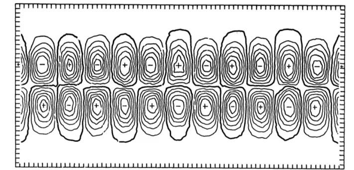
= .125, and the grid of Fig. 2.5.The error in the computed solution of 24/2t is shown in Fig. 3.4 for o = 1.7,
E
= .125 and grid of Fig. 2.5. The error consists of cells of alternating sign around the hemisphere with -egative error (computed minus analytic solution) west of the wave trough and positive west of the ridge. The maximum error of each cell is found between latitucs 20 and 25 0, the area of maximum vorticity advection. This type of error field produces a systematic underestimate of the true vorticity advection.Table 2 lists the largest positive and negative errors of 6fi/ t at time t = 0. These values are about 40 percent larger than the corresponding values from Gates and Riegel's integrations. Also, our results exhibit a larger and less systematic variation. The
actual error patterns are all like Fig. 3.4 for the other values of
ck and
E
tested.The errors in Table 2 and Fig. 3.4 are the accumulation of the errors of all the discrete approximations used. It is also of interest to examine the errors of each phase in the computation. We consider first the error in calculating the vorticity. Fig. 3.5 shows the vorticity field determined analytically. The error pattern from
calculating the vorticity from (3.2) esembles Fig. 3.5 closely, negative cells of error coinciding with positive cells of vorticity. This
implies that the values of calculated by the difference scheme are too small, and the gradient is smaller than it should be. The error is about 2.0 percent of the true values with grid orientaLion 1, and 2.4 percent with grid orientation 2. There is a slight distortion of the error pattern when a zero contour crosses a side of a major triangle.
The pattern of exact values of
3g/
t is like that of Fig. 3.4, but with uniform cells. The error in the Jacobian approximation using e::act values of and also resembles Fig. 3.4 with positive cells out of phase with those of ob /ot, indicating tarnt the values of V/3t are too smaLl. The error inat/
t is about 5 percent. When the values of obtained from (3.2)are used instead of the exact-32-Table 2 .25 .125 .0625 .65.5 -65.5 66.7 -66.9 69.0 -69.1 1.6 69.4 -69.5 66.5 -66.5 - -65.4 -65.2 67.5 -67.8 69.5 -69.7 1.7 67.9 -67.8 65.4 -65.5 64.3 -64.4 65.7 -66.4 68.9 -69.3 70.6 -70.8 1.8 63.4 -63.8 63.3 -63.5 63.5 -63.5 71.0 -71.7 71.4 -71.5 - -1.9 64.1 -64.9 63.9 -64.3 64.1 -64.1 2 -2
Maximum positive and negative errors of
by)/
t (m sec)
at t = 0. The upper numbers are for grid Fig. 2.4 the lower ones for grid of 'Tig. 2,5'.values, the error is increased to 13 percent. The error field is also more distorted at sides of major triangles in this case.
The values of
ai/
t were found by relaxing the exact field to compare with the values obtained in the previous section. The convergence properties are the same as those with the approximatebf/
t field. The error using exactaf9/t
values is 50 percent of that using the approximate 2f/ t values.3.4 Twelve day integrations
Initial conditions (3.4) were integrated for 12 days using 1 hour time steps,
d,
= 1.8,C
= .125, and the grid shown onFig. 2.5. The wave moved eastward without change of shape at a speed of 18.6 per day compared to 20 per day for the analytic solution. No figure showing the final field is included as the only observable difference between it and Fig. 3.2 would be the phase shift. The wave did not exhibit any tendency for the trough to tilt, as reported by Gates and Riegel (1965), even though the spherical geodesic grid is coarser with respect to the wave at higher latitudes.
Since the analytic solution to these initial conditions is simply a wave moving without change of shape,
q).)
integrated around latitude bands is constant witn time. Other quantities, such as kinetic energy and square vorticity, also have invariant zonal aver-ages for these initial conditions and, of course, invar ant global averages for arbitrary initial conditions. Examination of the -integrals of the numerical solution furnishes a good check on the
-34-accumulation of truncation error in the amplitude of the wave as a function of latitude. Fig. 3.6 shows a plot of
4)
integrated over the entire earth and also over two latitude bands. The middle curve is the average over the entire earth; the upper, for 50 to 600N, is typical for latitude bands above 40 ; and the lower, 20 to 30 N, is typical for latitudes below 400 with little variation near the equator. The averages are obtained by a simple summation of values at the points in a latitude band without weighting the values by the areas repre-sented by the points. The truncation error in this integration is not significant for this wave pattern.A small oscillation appears in all the averages with a period 0 of about 3.2 days. Since the computed wave moved with speed 18.6 per day, this oscillation can be attributed to truncation error depending on trough position with respect to the grid. To check the hypothesis, the same initial conditions were integrated for 12 days using a 10 degree grid (every other point of Fig. 2.5) with both one and two hour time steps. In both cases, the wave moved with a speed of 15 per day. The small oscillations again appeared in the averages with a period of 4 days, agreeing with the observed 15 speed.
If these small-scale oscillations are removed from Fig. 3.6, the mean is seen to increase in lower latitudes, decrease in higher latitudes, and remain steady over the whole globe for the 5 grid. These changes may be a manifevstation of truncation error being a function of latitude. Since the wave initial condition is a function of longitude increment, and the grid interval is a function of linear
increment, the grid is relatively coarser in high latitudes with respect to the field under consideration.
0
The integrations using- the 10 grid showed the means of all latitude bands increasing with time. The increase was very small for lower latitudes and increased to about 2.5 percent in 12 days for the
0
higher latitudes above 50*. The global average increased by less than 2 percent in the 12 days. The resolution of the 100 grid at high latitudes is quite poor with respect to the wave, there being slightly
0
less than four grid triangles per wavelength at 55 and obviously fewer at higher latitudes.
An initial condition of wave number four was also integrated over the 5 degree grid of Fig. 2.5 using 1 hour time steps. The
initial condition is that given by Phillips (1962) as
=
-318.45
Sin
W
+318.45
cos'cp
Sirp
cos
4 \
(3.5)2 -1
in units of km sec . Such a wave moves eastward with a speed of 12.2 degrees per day. Again the actual final pattern after 12 days did not differ significantly from the initial pactern except for the phase shift.
In this case the trunc-:tion error in approximating the inte-gration of 4)2 by an unweighted average over grid points is no longer negligible. Continuous integratiorn of would result in constant zonal averages. However, when the analytic values are summed only at grid points, the result (solid curves in Fig. 3.7) is
-36-seen to vary with a period of about 7.4 days. Such a period cor-responds to the pattern moving one wavelength with respect to the grid. The averages of the numerical solution are given as the dotted curves in Fig, 3.7. The slightly larger period of the nu-merical solution is caused by the phase truncation error of the scheme. If the truncation error associated with the integration over latitude bands is subtracted, the same comments can be made concerning the truncation error of the model as in the wave number six case.
4
A4
P
25PO3
3
P
5IB
C
2
P2
Fig. 3.1 Grid triangles and points for difference equations.
J 1 1 1 1 1 1 1 1 11 i11 1 i11I 1 11 1 11 1 1 1 i 1 1 1 1 1 1 1 1 111 1 1 1 1L
-21
...-
14
011110
+7
+14
+ 21
Fig. 3.2 Initial wave number six field. Intersections of 50 latitude,
longitude lines are projected onto a rectangular grid for the figure. The equator has zero 4) value,. Contour Interval is 3.5x10⁷ m2 sec .
150
140
130
120
11O
100
90
80
70
60
50
40
30
20
1.4
1.6
1.8
2.0
OVER RELAXATION COEFFICIENT
Of
Fig. 3.3 Convergence speed of relaxation. Dashed lines are for the grid of Fig. 2.5, solid lines are for that of Fig. 2.4. The desh-dot line is a corresponding curve from Gates and Riegel converted to our coor-dinates.
4 0
~.Ji....1L||||.L. .Jiii I11 I I I I I I I I I I I I I I I I I I I I I I I I I I I I I| I I I I I I I I I I I I I I
-Fig. 3.4 21/ t error at time t=0, 0
=
1.7,6
= .125, and for grid of Fig. 2.5.Fig.
3.5 Exact values at time t= 0. The dark line is the zero contour; contour intervalis 7x10⁻⁶ sec
1.
The) figure was produced by the computer using linear interpolationwithin grid triangles. This causes the small irregularities in this and previous figures.
-42-N*0
CM
eD 2.7 000 o ee*'eTO~TAL __ .*.. .. .----.... *..--'"--....-' --- T TA x2.6
6.o..-
20- 30*1.4
0
2
4
6
8
10
12
DAYS
Fig. 3.6 Variation in
)
averaged over the entire earth and within the latitude bands 20-300N and 50-60 0N for wave number six.Variation in averaged in latitude bands and over entire earth. The ordinate is (xlO16 m4 sec -2). The dotted lines are for numerical integration of wave number four. Solid lines are for analytic values
indicating truncation error in the integration over latitude bands as opposed to truncation error in the model itself.
8.
8.
8.
6.9-6.70 5.00
0
27
0
1
3D.YS
5.2
52. 3
-
-*o *
* o
5 . O
3.06
30.9
.-3 . ' T -- l 0 ,6
.0 -1-.
A.*
CHAPTER IV
PRIMITIVE BAROTROPIC MODEL ON A PLANE
We digress from the sphere for one chapter to consider differ-ence approximations on a plane. Here we develop methods of approx-imation over triangular grids which will be useful to compare trian-gular approximations with the more usual square ones. Obviously, if triangular approximations are significantly worse than the square ones there would be no point in proceeding to the sphere. These
schemes on the plane also have a side benefit for use as nonhomogeneous grids to deal with problems with spatially varying scales of motion.
The spatial scale of many geophysical fluid dynamics problems varies greatly over the domain of interest. The ocean circulation is such a problem. Western boundary currents such as the Gulf Stream or Kuroshio have a smaller scale than the remaining ocean circulation.
Another example is the problem of fronts in the atmosphere, where relatively strung gradients exist in a narrow band with weak gradients elsewhere.
To study these problems numerically, a net of points must be defined over the domain. The density of the net must be great enough to resolve the smallest scales of interest. The size and speed of present computers does not allow a uniformly fine grid over the entire domain. Even if it were practical, such a grid would be inefficient since a fine grid is needed only over a small part of the domain.
-45-For efficient use of the computer, it seems reasonable to use the optimum grid density for the spatial scale of the expected solution in each part of the domain. These various density grids must then we connected to each other in some manner and, in some cases, special difference equations must be designed for use at the interface.
If a coarse square grid is joined to a fine square grid, various difficulties can arise at the interface. For example, if a uniform wave is travelling parallel to the interface, the phase truncation error is smaller in the fine grid than in the coarse one, and a shearing soon develops in the wave structure. This numerical phenomenon is exhibited in the case of a wave on a sphere by Gates and Riegel (1962). If a wave is moving perpendicular to the inter-face, partial reflections might occur which are due solely to the numerical techniques and not to the physical problem.
To avoid these problems, a nonhomogeneous triangular grid seems ideal. Such grids have been used successfully for solving elliptic equations by the method of successive overrelaxation
-(Winslow, 1966). Thoy permit a continuous, gradual transition from fine to coarse grid and permit construction of secondary polyhedral grid areas whose sides are common to only two such areas.
Masuda (1968) has developed finite difference schemes using the principle developed by A. Arakava for use over a homogeneous triangular grid. He shows good results for integrations of the non-divergent barotropic model on a plane. Lorenz (1967) has developed
a finite difference approximation for a two level model on a beta plane when the governing equations are written in terms of a stream function. In the following, discrete approximations to the primitive equations governing frictionless two-dimensional flow are developed
for use over arbitrary triangular grids. Cartesian geometry is assumed for this chapter. The modifications necessary for spherical geometry are discussed in Chapter V. Two approaches are considered. The first deals with the invariants of the continuous equations. A class of schemes is developed which conserves mass, momentum, and energy. The second approach approximates each term of the governing equations individually and examines the truncation error of all the
schemes when applied to a homogeneous grid over a plane.
Results of test integrations of these schemes are then pre-sented. The schemes are applied to an equilateral triangular (homo-geneous) grid on a beta plane. No integrations over nonhomogeneous grids are performed. The results of the triangular schemes are compared with results of similar schemes applied to a square net and with results of integrations over a fine mesh.
The equations considered here are those for frictionless hori-zontal two-dimensional motion. For the derivation of the difference schemes, the Coriolis term will be neglected. Since all quantities will be defined at the same grid points, the Coriolis term can be
differenced in a straightforward manner. The difference form of the Coriolis terhi is given in section 4.7. Using vector notation, the
-47-governing equations can be written
+
v.;v
+~?~
(4.1)
- V .ekV :(4.2)
where
V
is the vector velocity, h is the height of the free surface, g is gravity, and7
is the vector gradient operator. Equation (4.2) expresses conservation of mass.The momentum equation can be formed from (4.1) and (4.2), and, using diadic notation, can be written as
) +(4.3)
Thus, neglecting boundary effects, the system conserves momentum when integrated over the domain. The kinetic energy equatiion is obtained by combining (4.1) multiplied by
V
with (4.2) mult iplicd by \V.\V V Z/.. V- =- (4.4)
This equation, together with gh times equation (4.2) yield:6 the energy equation
The total energy
(
-\/
+
k')
is seen to be conserved when
integrated over the domain with boundary effects neglected.
We now wish to develop difference approximations to these partial differential equations and study their properties. Such approximations are easiest to develop from area integrals of the flux form of the equations. Consider integrals of equations (4.2) and (4.3) over some elementary grid area A yet to be defined.
i
JA
-('JA
-VKJA (46A
A
A
-,*11)C -(4.7)
tSk
JA
O-x(I
TJA
A
A
The area integrals on the right hand side can be transformed to line integrals along the boundary S of A.
---
k\V
cA
=
-
/
\
ls-
g
--
A
cS
(4,8)
2A
S
5
S (4.9)A
AWhere Vn is the velocity component normal to the curve S and n is the outward unit vector normal to S.
-49-4.1 Conservative difference schemes
The difference schemes developed here are all written for a topologically regular grid in the sense that each grid point is surrounded by six triangles. Difference equations expressing the
change of a variable at a grid point are written using local polar indexing. The value of some variable
)
at a central point is denoted by 0 . The values at surrounding points are thendenoted by ( /'( . /.' is the row radius of the
point; i=1 for a grid point one triangle from the center, 2 for a point two triangles out, etc.
eg
is the azimuthal angle,0
j
= 1 for some reference line, 2 for a point 60 counterclockwise on a topological map of the grid, 3 for a point 120 , etc. See Fig. 4.1.With this notation, a set of difference approximations to equations (4.8) and (4.9) conserving mass and momentum is given by
.. (4.10)
jai
41
A~ik
0
(4.11)
A is the area of the hexagon whose sides go through and are
0 CZ
perpendicular to the grid lines, is the length of the side
and is the velocity component normal to the side.
(kL2)A
,and(V\
)
are to be related to grid point9 2
values from energy considerations.
Let q) denote the finite difference equivalent of inte-gration of a quantity
Y
over the domain, i.e.,y=
LA.9.
where the summation is taken over all grid points, and AT is the total area.
In order for (4.10) and (4.11) to conserve energy, the follow-ing relations must hold
2
\ V (4.12)As$
ZA (4.13)
The first relation (4.12) insures that the space differences will not produce nonlinear instability; the second (4.13) provides for
-51-If we define
( , h)j
.
-=O
,
(4.14)equation (4.12) holds because
6a
(otk
*V~~jL
Avj~
=0
Differences with the form of (4.14) have been used by Lorenz (1960), Arakawa (1966), and Bryan (1966).
One possible definition of
M 1(4.15)
The energy conversion relation (4.13) then holds provided that
( AD
(4.16) =
Substitution of (4.14), (4.15), and (4.16) into (4.10) and (4.11) results in one energy conservative difference scheme given as
Scheme I 4
A
OZADLi
Y
7v
2A,
II
0j
1
7
A
2A..
If applied to a square grid this scheme is seen to be the same as scheme B of Grammeltvedt (1968).
A second possible definition of
(
,
** A
(4.18)
Relation (4.13) is now valid if
(a t
2
Substitution of (4.14), (4.18), and (4.19) into (4.10) and (4.11) results in a second energy conservative scheme given by
4A*
(4.17)(4.19)
eO
O
Aa
-53-Scheme II
A %
(4.20)
A..
We note that the mass flux of Scheme I is similar to Shuman's (1962) semi-momentum scheme and that of Scheme II is similar to his filtered factor form. These two schemes are also similar to those designed by Kurihara and Holloway (1967) for use over a quasi-homogeneous spherical grid.
4.2 Individual approximations
Difference approximations are now formulated for the individual terms of the governing equations without regard to energy conserva-tion. First, grid vectors which are useful in writing the approxima-tions are defined.
Let S. be the vector from the center point 0 to the surround-ing point (1,1) (sc Fig. 4.2a). The r-dil ubri is now dropped, all points considered being in the first row around the center point.
Two adjacent points along with the center point form a triangle
with values
J
and
of some field
(
at its
vertices. IfY
varies linearly over this triangle it can bewritten, following Winslow (1966), as
-- % (4.21)
where the gradient is a constant within the triangle and given by
S is the position vector with respect to the center point, and the 0
superscript T denotes a 90 clockwise rotation of a vector (Fig. 4.2a).
A proof of (4.22) is straightforward. Since I4 is assumed to vary linearly in the triangle, it can be written in the following torm
where f and g are vector functions of S. and Si+1 . Since
C kl -- -- b -..
Yit follows that S -f = 1 and S g = 0.
-- -3 - --%
Similarly
.
(
+
-(
implies
f
1 and Si+1
Thus f and g have the form f CS.r and g= C ST where
.i.+l 2 i
-55-Define a secondary mesh for the grid to consist of the medians of the grid triangles (Fig. 4.3a). The elementary grid area associated with each grid point is then that of the secondary dodecagon surrounding it.
Pressure Gradient Term
Consider the integral of the pressure term over the dode-cagonal grid area of Fig. 4.3a
A
and assume h varies linearly within each of the six grid triangles. The contribution to the integral from the area C formed by the intersection of one grid triangle and the dodecagon is
where the position vector S is the only variable in the integral. Hence
In the grid triangle defined by S is that of the two triangles defined by
is
and S , the area i+l
and I~l+)
9 (sil + i)1 and -(S + .)
3
i+l i andiS
1+ 1 (see Fig. 4.3b). In these twotriangles, is and
v
* Thus12
;I-l:;;71~~.
z-a:s
with the above values substituted.
Similarly, other approximations to the pressure term can be defined. Consider the integral
3
z
A and let h
then becomes
vary linearly over the grid triangles. The integral
;4-
-57-where the expression for the gradient is given by (4.22).
Another approximation can be formulated from
22
where h is assumed to vary linearly over grid triangles. In this case the line integral becomes simply the trapezoidal rule with values at the vertices of the dodecagon. The integral 14 can be evaluated other ways, such as by assuming h varies linearly over grid triangles. The line integral doos not reduce to the trapezoidal rule in this case.
Mass Flux
Difference approximations for the mass flux term, right hand side of (4.23), are now considered:
__ _ (4.23)
Let
V
vary linearly within grid triangles. The two outward normals along the two sides of the dodecagon (see Fig. 4.3b) within the grid triangle defined by S. and S. are given by1 i+1
and
A 2.
A A
Substituting these expressions for n and n , plus equations (4.21)
1 2' u
and (4.22) for
V
into equation (4.23) along with somemanipula-tion, leads to the difference equation
---
-'
-
T (4.24)A,
Another approximation can be derived by assuming both h and
V
vary linearly over grid triangles and approximating the line integral in (4.23) with the trapezoidal rule between vertices of the dodecagon. This approximation becomes-~
72z
A*[v
b~
Ys.,-i
(4.25)
CT
Awl
Other approximations can be found by making assumptions similar. to those made in approximating the pressure gradient term.
-59-Momentum Flux
Approximations for the momentum flux term on the right hand side of the following equation
(4.26)
kt A
A
(VJ
V
A
can be obtained using the same methods as the mass advection. For example, if
V
V
is assumed to vary linearly within gridtriangles, the resulting expression for (4.26) becomes
6
(4.27)1 -- I
By making approximations similar to those made for the mass flux, other difference schemes can be obtained.
4.3 Homogeneous grid
We now consider the form these schemes take when applied to an equilateral triangular (homogeneous) grid and determine the cruncation error of such approximations. Consider Cartesian
coor-A
dinates (x, y) with unit vectors ' .,
j
) . LetO
be the constant distance between grid points, and define the grid vectors S. byS
£3S4
VA A..2 .
3
A.
2
See Fig. 4.4.Consider first the pressure term on the right hand side of the following equation
,V)
I'
A(,
or an equivalent form. We denote discrete approximations to the right hand side as P Since