HAL Id: inria-00539874
https://hal.inria.fr/inria-00539874
Submitted on 25 Nov 2010
HAL is a multi-disciplinary open access
archive for the deposit and dissemination of
sci-entific research documents, whether they are
pub-lished or not. The documents may come from
teaching and research institutions in France or
abroad, or from public or private research centers.
L’archive ouverte pluridisciplinaire HAL, est
destinée au dépôt et à la diffusion de documents
scientifiques de niveau recherche, publiés ou non,
émanant des établissements d’enseignement et de
recherche français ou étrangers, des laboratoires
publics ou privés.
Scheduling, Binding and Routing System for a
Run-Time Reconfigurable Operator Based Multimedia
Architecture
Erwan Raffin, Christophe Wolinski, François Charot, Krzysztof Kuchcinski,
Stéphane Guyetant, Stéphane Chevobbe, Emmanuel Casseau
To cite this version:
Erwan Raffin, Christophe Wolinski, François Charot, Krzysztof Kuchcinski, Stéphane Guyetant, et al..
Scheduling, Binding and Routing System for a Run-Time Reconfigurable Operator Based Multimedia
Architecture. Design and Architectures for Signal and Image (DASIP), Oct 2010, Edinburgh, United
Kingdom. �inria-00539874�
Scheduling, Binding and Routing System for a
Run-Time Reconfigurable Operator Based
Multimedia Architecture
E. Raffin∗¶, Ch. Wolinski∗†, F. Charot†, K. Kuchcinski§, S. Guyetant‡, S. Chevobbe‡and E. Casseau∗†
∗University of Rennes I. Rennes, France. Email: [email protected]
†INRIA. Rennes, France. Email: [email protected]
‡CEA, LIST. Gif-sur-Yvette, France. Email: [email protected]
§Dept. of Computer Science, Lund University, Sweden. Email: [email protected]
¶Technicolor Research & Innovation, Rennes, France. Email: [email protected]
Abstract—This paper presents a system for application scheduling, binding and routing for a run-time reconfigurable op-erator based multimedia architecture (ROMA). We use constraint programming to formalize our architecture model together with a specific application program. For this purpose we use an abstract representation of our architecture, which models memories, re-configurable operator cells and communication networks. We also model network topology. The use of constraints programming makes it possible to model the application scheduling, binding and routing as well as architectural and temporal constraints in a single model and solve it simultaneously. We have used several multimedia applications from the Mediabench set to evaluate our system. In 78% of cases, our system provides results that are proved optimal.
Keywords-Constraint Programming; Reconfigurable Architec-tures; Embedded Platforms for Multimedia;
I. INTRODUCTION
Nowadays, modern highly parallel architectures are com-posed of many parallel processing units (homogenous or heterogenous) connected through communication networks. The processing elements are usually equipped with local memories. For about ten years, they have been containing, more and more frequently, run-time reconfigurable data-paths well tailored for selected classes of specific applications. These architectures are very efficient but tools to compile application programs for these new application-specific architectures are still missing. To do application scheduling, binding and routing for such systems is not a trivial task. To tackle this problem, we proposed a new generic system based on the constraint programing paradigm (CP) that enables execution of all above discussed tasks simultaneously. For the purpose of this paper, our system was adopted to support a run-time reconfigurable operator based multimedia architecture (ROMA).
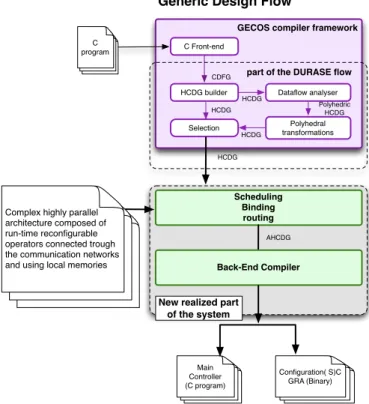
The general flow of the proposed system is presented in Figure 1. It uses a generic compilation platform GECOS recently extended with polyhedral transformations [1]. Our system uses Hierarchical Conditional Dependency Graphs (HCDGs) as the internal design representation. HCDG cap-tures both the application control-flow and data-flow [2], [3]. It supports formal graph transformations and optimizations.
GECOS compiler framework
Scheduling Binding routing
C Front-end
HCDG builder Dataflow analyser
Polyhedral transformations Selection CDFG HCDG HCDG Polyhedric HCDG HCDG HCDG
part of the DURASE flow
C program
Generic Design Flow
AHCDG
New realized part of the system Main Controller (C program) Configuration( S)C GRA (Binary) Back-End Compiler
Complex highly parallel architecture composed of run-time reconfigurable operators connected trough the communication networks and using local memories
Fig. 1. Global design flow overview.
In the HCDG, graph nodes are guarded by boolean conditions and polyhedrons depending on loop indexes and parameters. After data-flow analysis [4], each read statement in a graph has a set of possible source contributions relying on its execution contexts and polyhedral conditions. Finally, loops are unrolled totally or partially to generate an HCDG which is an input to the remainder part of the system.
As shown in Figure 1, the inputs to our system are an application program written in C and an abstract generic par-allel run-time reconfigurable architecture model. The outputs are the C program and the configuration information (binary files) needed to manage the run-time reconfigurable ROMA
architecture.
The newly developed system, presented in this paper, is part of the DURASE system [5], [6] (see Figure 1). It implements our new method, based on CP, that enables to model complex run-time reconfigurable architectures together with their application programs. The model can then be used to perform scheduling, binding and routing while optimizing application’s execution time. Our system contains also the tar-get dependent back-end compiler (in our case, the supporting ROMA architecture).
This paper is organized as follows. In section II, related works on scheduling and mapping are discussed. The targeted architecture and its abstract model is presented in section III and III-E. Section IV introduces briefly constraint ming, that is used in our approach. The constraint program-ming model to solve the resource constraint scheduling, bind-ing and routbind-ing simultaneously for the abstract architecture model is discussed in V. Section VI presents experimental results. Finally, conclusions are presented in section VII.
II. RELATED WORK
Application scheduling, binding and routing for a run-time reconfigurable architectures are complex problems. Each of these problems is known to be NP-complete. In general two trends are dominant to deal with these kind of problems, both coming from high-level synthesis (HLS) domain.
First trend represents simple and dedicated algorithms to solve practical instances of the problem effectively and effi-ciently. List scheduling, for example, and its derivatives are the most commonly used and adapted algorithms. In [7], near optimal results are obtained quickly using a list-based scheduler thanks to a tight cohesion between partitioning and scheduling steps. More recently, [8] targets an industrial distributed reconfigurable instruction cell based architecture considering binding and routing effect, register assignment and operation chaining. Branch-and-Bound algorithm have been proposed in [9] and delivered good results but addressing scheduling and allocation separately.
Second trend represents methods for solving these problems optimally. Integer linear programming (ILP) and Mixed integer programming (MIP) are common methods for mixed con-strained version of these problems. They are also frequently used to compare results from heuristic-based methods. The contribution presented in [10] is particularly in line with our work because an ILP formulation for solving optimally and simultaneously the mapping, routing and scheduling of a given data flow graph on a coarse-grain architecture is presented. The main difference, apart the formulation type, resides in the targeted architecture model, which consists of homogeneous processing elements and mesh-like interconnection network. In [11], a MIP formulation is proposed for optimal mapping of digital signal processing algorithms on commercially VLIW DSPs, both homogeneous and heterogeneous architecture are addressed.
The constraint programming (CP) approach is one of the most relevant in the second trend and particularly developed
during last years for different purpose. Kuchcinski and Wolin-ski, have widely participated in this development through their research, mainly in HLS [3], [12], [13]. More recently they also contributed to generation of optimized application specific reconfigurable processor extensions [14], [15]. This approach has also been used in the context of embedded distributed real-time systems [16].
According to a recent survey on methods and tools for embedded reconfigurable systems [17], CP and evolution-ary/genetic algorithms presented in [18] belong to the most promising approaches to efficiently produce high-quality so-lutions for the complex architecture synthesis problems in-volving multi-objective optimization. To illustrate this, [19] compares three static schedulers. First one, list-based, has high efficiency but the least accuracy; the second, based on CP, ensures optimal solutions but with significant searching effort; the last one, based on a genetic algorithm, shows reasonable efficiency and better accuracy than the first one.
To our knowledge, this is the first paper addressing the prob-lem of solving simultaneously binding, routing and scheduling a data flow graph for the run-time reconfigurable operator based embedded architecture using CP. With this approach, it is possible to solve simultaneously application binding, routing and scheduling problems under architectural and temporal constraints. Moreover, we use the JaCoP solver [20], which provides classical primitive constraints but also conditional and highly efficient global ones particularly useful for our problem formulation.
III. DESCRIPTION OFROMA PROCESSOR
The ROMA processor is composed of a set of coarse grain reconfigurable operators, data memories, configuration mem-ories, operator network, data network, control network and a centralized controller. The centralized controller manages the configuration steps and the execution steps. The ROMA processor has three different interfaces: one data interface connected to the operator network, one control interface and one debug interface connected to the main controller. A. Reconfigurable datapath
The reconfigurable datapath of the ROMA processor is made up of a set of heterogeneous or homogeneous recon-figurable operators. Their number can be statically changed from 4 to 12 depending on the computing power needed for a particular application domain. Each reconfigurable operator has its own configuration memory and its own control interface to the main controller, each of them being able to be configured and controlled independently.
These reconfigurable operators are connected together via a dedicated network (called operator-operator network) and to the data memories via another network (called data memory-operator network). The local memories have their own pro-grammable address generators. Figure 2 shows the block diagram of the ROMA processor. The main controller (Global CTRL) executes a C program defining synchronisations be-tween the configuration and execution sequences.
!"#$%&'$( !"#$%&'""$()'"*"$#+'%, )%&% *#+ ,-(& *#+ ./'0%/ 1234 )#056 ,7 !-./012 &#%3 45*&#%3 26 &#%3 1&$/ ,7 27$%8#'%*9*'7$%8#'% :8#8*;$;'%<*9*'7$%8#'% 26= 26> 26? 26@
1AB 1AB 1AB 1AB )%&%8+#+'$980%-:( :8#8 C8", 45 :8#8 C8", 45 :8#8 C8", 45 :8#8 C8", 45 :8#8 C8", 45 :8#8 C8", 45 )%&% ,7
Fig. 2. Architecture of ROMA processor : the control structure includes
a Global CTRL and dedicated controllers designated for each module of the reconfigurable datapath. The reconfigurable datapath is composed of data memory banks, two interconnection networks and a set of coarse grain reconfigurable operators.
B. Coarse grain reconfigurable operator
The coarse grain reconfigurable operators are four pipeline stage operators that can execute standard arithmetic (such as ADD, SUB, MUL, ABS), logic (such as AND, OR, XOR) and shift operations. The operators can also compute accumulation operations (such as SAD and MAC). The datapath of the operators has 32/40 bit wide inputs and outputs. The multiplier is a 16x16 bit multiplier that can be split into two 8x8 bit multipliers.
C. Interconnection networks
The transfers inside the ROMA processor are organized according to the type of communication. There are data, con-figuration and control communications and the interconnection networks were split according to these types. These intercon-nection networks allow partial reconfiguration, to prepare the next communication pattern without stopping the execution. The interconnection networks are configurable in one cycle. D. Data interconnection network
The data transfers can be done either between data mem-ories and operators or between operators themselves. Dedi-cated interconnection networks were designed to connect data memories to operators (data memory - operator network) and operators together (operator - operator network). The data width is parametrizable between 32 bit and 40 bit according to the needs. The data interconnection does not add any clock cycles during the communication, but a fixed latency between 1 and 3 cycles according to the number of operators and data memory banks. A communication pattern is defined by two configurations, for both types of networks. The goal of this solution is to minimize the hardware complexity of the interconnection network and avoid a costly crossbar intercon-nection.
Data memory - operator interconnexion network
Op
...
Op Op...
Memory Memory Memory
Operator - Operator interconnexion network
Fig. 3. Generic architecture model.
1) Operator - operator interconnection network: The op-erator - opop-erator interconnection network is able to achieve all acyclic connection patterns between reconfigurable oper-ators, connecting N operators with 2 inputs and 1 output. This interconnection network is optimized to minimize the hardware cost and the latency. Each output of each operator can be connected to each N/2 inputs of the next operators (i.e., operators with higher identification number). An output can be connected to several inputs of the next operators. Each connector is configured by one bit.
2) Data memory - operator interconnection network: The data memory - operator interconnection network has to support connections between data memory banks and the operators and can achieve several communication patterns simultaneously. This flexibility is needed to ease the data placement in the data memory banks. This interconnection network should minimize the critical path. Thus, 1 to 3 latency cycles are needed to cross the data memory - operator interconnection network. These latency cycles are managed during the compilation of an application. The latency is variable according to the distance between the memory bank and the operators that are connected.
E. Architecture Abstract Model
The abstract architecture model of the ROMA architecture is depicted in Figure 3. It is composed of local memories, a memory-operator interconnection network, reconfigurable operators and a specific operator-operator interconnection net-work. The architecture is defined as follows.
• the number and size of the local memories are
parametrized,
• each memory has one true port; it means that only one
read/write operation can be executed at the same time,
• the read/write operation latencies are constant,
• each memory is identified by a unique number,
• each operator is identified by a unique number,
• the operators can be heterogenous (each operator can
execute a specific set of complex operations),
• each operator has at most two input ports and one output
• the memory-operator interconnection network is a full
crossbar network,
• the operator-operator interconnection network is
parametrized; it can be defined by a connection matrix containing the information about point to point operator connections,
• the operator-operator interconnection network is
charac-terized by a constant read/write latency.
This abstract architecture has been implemented in our framework as a meta-model with its own editor allowing easy and quick specification of the resource constraints. In this way, it is possible to specify the amount of functional resources and supported operations, each with a delay, amount of memory, etc.
IV. CONSTRAINTPROGRAMMING
In our system, we use constraint satisfaction methods im-plemented in constraint programming environment JaCoP [20], [21]. Below we provide a very short introduction to constraint programming but the more thorough discussion can be found in [22], for example.
A constraint satisfaction problem (CSP) is defined as a 3-tuple
S = (V, D, C) where V = {x1, x2, . . . , xn} is a set of
vari-ables, D = {D1,D2, . . . ,Dn} is a set of finite domains (FD),
and C is a set of constraints. Finite domain variables (FDV) are defined by their domains, i.e. the values that are possible for them. A finite domain is usually expressed using integers, for
example x :: 1..7. A constraint c(x1, x2, . . . , xn) ∈ C among
variables of V is a subset of D1× D2× . . . × Dn that restricts
which combinations of values the variables can simultaneously take. Equations, inequalities and even programs can define a constraint.
A solution to a CSP is an assignment of a value from variable’s domain to every variable, in such a way that all constraints are satisfied. The specific problem to be modeled will determine whether we need just one solution, all solutions or an optimal solution given some cost function defined in terms of the variables.
The solver is built using constraints own consistency methods and systematic search procedures. Consistency methods try to remove inconsistent values from the domains in order to reach a set of pruned domains such that their combinations are valid solutions. Each time a value is removed from a FD, all the constraints that contain that variable are revised. Most consistency techniques are not complete and the solver needs to explore the remaining domains for a solution using search. Solutions to a CSP are usually found by systematically as-signing values from variables domains to the variables. It is implemented as depth-first-search. The consistency method is called as soon as the domains of the variables for a given constraint are pruned. If a partial solution violates any of the constraints, backtracking will take place, reducing the size of the remaining search space.
The constraint programming approach has been recently used in UPaK (Abstract Unified Patterns Based Synthesis Kernel for
Architectural constraints
AG
Abstract Architecture Model
Coarse Grain Operator library C program Resource constraints Main Processor Program (C) CGRA Configuration(S ) (Binary) Graph too big ? Parallelism degree Constraints Structural Analysis Graph Covering using accumulation patterns Mapping Constraint (# config = 1) NOT mappable in 1 configuration Main Processor Program (C) CGRA Configuration (Binary ) Multi-Scheduling Binding Clustering Scheduling Binding No solution Control Unit
RPU0 ?1 RPUN-2 RPUN-1
$0 $1 $M-2 $M-1 Routing Routing Back-end Compiler ROMA Design Flow Front-End
Fig. 4. Detailed scheduling, binding and routing and flow. Hardware and Software Systems) [15] for automatic design of application-specific reconfigurable processor extensions.
V. SCHEDULING ANDBINDINGCONSTRAINTMODEL
The place of scheduling, binding and routing steps in the whole design flow are presented in detail in Figure 4. The inputs for these steps are the application graph (AG), the library of the functionally reconfigurable operators and the architectural constraints (derived from the ROMA multi-media architecture). The outputs are the main processor program (C file) and the configuration information (binary files).
The ROMA architecture supports two modes of execution. The first one corresponds to the data flow model of execution. This mode can be used when only one configuration is used during the processing. In the second mode, the configuration of the communication networks and configuration of operators can be changed each cycle. In this paper, we consider both modes of execution but the accumulation operations available in mode one are not considered.
A. Application Graph
Formally, the AG is modeled as a direct acyclic graph AG = (N, E) where each node n ∈ N represents a computation
(n ∈ OPs) or an input/output memory access (n ∈ IOs) and
each direct edge e ∈ E a data transfer. B. Finite Domain Variables Definition
In order to model the scheduling, binding and routing we use the following primary FDVs defined for all nodes n ∈ N and all edges e ∈ E.
• nstart :: {0..∞} defines the start time of processing of
• ndelay defines the processing time of node n (in the
ROMA processor an execution time of node n is constant for all reconfigurable operators),
• nend :: {0..∞} defines the processing completion time
of node n,
• nop :: {i|opi ∈ {0..|operators| − 1} ∧ opi can execute
n} defines the operator binding to node n,
• nopactivity :: {0..∞} defines the time when operator op
is occupied to execute node n ∈ OPs; this time includes
node processing time and the time needed to transfer the data,
• nmem :: {0..|memories| − 1} defines the memory used
to store the data from node n,
• nstartW R :: {0..∞} defines the starting time of the
memory data write operation for the data coming from node n,
• eijstartRD :: {0..∞} defines the start time of the memory
data read operation for the computation represented by
node nj, (data produced by node ni),
• nstoreMn :: {0, 1} defines whether the data from node n
needs to be saved in memory Mn(value 1) or not (value
0),
• nlif e_time :: {0..∞} defines the life time of the data
produced by node n,
• emem_ope :: {0, 1} defines whether the memory-operator
interconnection network is used (value 1 ) for the data transfer represented by edge e,
• eope_ope :: {0, 1} defines whether the operator-operator
interconnection network is used (value 1) for the data transfer represented by edge e.
Secondary FDVs variables are introduced, when needed, later in this paper..
C. Communication Constraints
In AG, an edge represents a data transfer on one of the two communication networks, either through the memory-operator interconnection network or through the memory- operator-operator interconnection network. For each edge e ∈ E we define exclusive choice of the network using constraint (1).
∀e ∈ E : emem_ope+ eope_ope= 1 (1)
If an edge represents a data transfer from an input node to a computation node, then we impose constraint (2) to use the memory-operator interconnection network. Similar constraints are imposed for data transfers from a computation node to an output node.
∀eij = (ni, nj) ∈ E|ni∈ IOs ∧ nj∈ OP s∨
ni ∈ OP s ∧ nj∈ IOs :
ei,jmem_ope= 1 (2)
In the ROMA architecture, the memory-operator intercon-nection network is implemented as a full crossbar network. For this reason we do not need to impose any additional resource sharing constraints to model these connections.
On the contrary, the operator-operator interconnection net-work imposes some communication limitations according to the network topology presented in III-D1 and III-E. In this
case, constraint (3) must be fulfilled for each edge eij =
(ni, nj) ∈ E when ni, nj∈ OP s.
If eijope_ope = 1 then njop= niop+ eijopr (3)
Note that we introduced variable eijopr :: {1..|operators|2 } for
all edges. This variable models which operators (represented
as operators’ numbers) are reachable from operator niop. The
finite domain of this variable can be equal to {0..|operators|
2 }
if a loop back link on operator exists.
In general, to model the topology of a specific network, a dedicated communication matrix ComMat can be used.
This matrix represents a relation between nodes niopand njop
and contains information about all possible point to point connections between these nodes. In this case, constraint (3) is replaced by constraint (4). In practice, it is implemented as
ExtensionalSupportconstraint [21].
Ifeijope_ope= 1 then njop= ComMat[niop] (4)
D. Timing Constraints
The completion time of the processing of node n ∈ OP s
(nend) is defined by equation (5). Note that if n ∈ IOs then
ndelay= 0.
nend= nstart+ ndelay (5)
The node precedence relations imposed by the partial order of AG are modeled by constraints (6) or (7) depending on which communication network was selected for data transfer.
In order to transfer the data between two nodes ni, nj ∈
OP s (ei,j = (ni, nj) ∈ E ) through the memory-operator
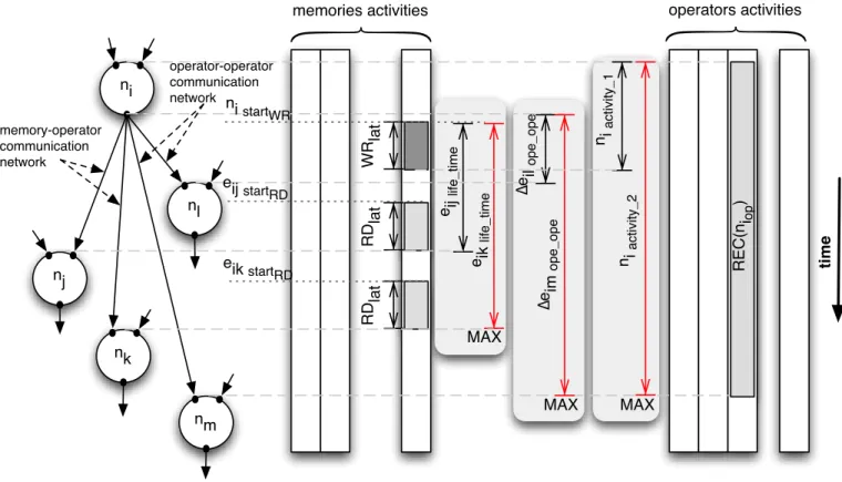
communication network, memory write and read operations must be modeled (see Figure 5). In the ROMA architecture, each operator produces one result that can be communicated to other nodes. Therefore, only one memory write operation for all output edges is modeled. The memory read operations
are modeled for each out-coming edge e ∈ noutputsusing the
memory-operator communication network for data transfers. The start times of memory write and read operations are
modeled by FDVs nistartW R for all nodes ni ∈ N and
ei,jstartRD for all edges from ni, respectively. Inequality (6a)
constraints the start time of a memory write operation in relation to the completion time of the operation represented
by node ni. In the same way, the memory read operation of
the previously saved data is defined in constraint (6b). In this case, the read operation takes place when a corresponding write operations is completed. Finally, the next operation can begin only when its input data are loaded (constraint (6d)). The delays of both memory write and read operations,
∆eijW R and ∆eijRD, are computed using constraints (6c) and
ni nl nj nk nm WR lat RD lat RD lat
memories activities operators activities
ni startWR eij startRD eik startRD e ij life_time e ik life_time MAX MAX MAX ! e im ope_ope ! e il ope_ope n i activity_1 n i activity_2 REC(n iop ) memory-operator communication network operator-operator communication network time
Fig. 5. Example with communications on both networks.
read latencies (denoted W Rlat and RDlat) derived from the
architecture model and the constants considered here.
nistartW R ≥ niend (6a)
eijstartRD ≥ nistartW R + ∆eijW R (6b)
∆eijW R = W Rlat∗ ei,jmem_ope (6c)
eijstartRD + ∆eijRD = njstart (6d)
∆eijRD = RDlat∗ ei,jmem_ope (6e)
The precedence constraints between nodes ni and nj ∈
OP s (eij = (ni, nj) ∈ E) imposed when a data transfer
is done through the operator-operator network are specified
by formulas (7), where FDV ∆eijope_ope :: {0..∞} represents
the time when the network is occupied. We consider that the operator-operator interconnection network is occupied from
the completion time of the processing of source node ni
to the start time of the processing of destination node nj.
This is formalized by (7a). In (7b) the operator-operator
interconnection network latency ope_opelat, derived from the
architecture model is used to constrain the occupation time.
Variable ninet_acces = 1 if at least one data transfer through
the operator-operator interconnection network is executed.
∆eijope_ope= njstart− niend (7a)
∆eijope_ope≥ ope_opelat∗ eijope_ope (7b)
ninet_acces ∈ {0, 1} ⇔
�
∀eij∈nioutputs
eijope_ope> 0 (7c)
E. Resource Sharing Constraints
In our CP model, we model the resources sharing process
by using the combinatorial constraintDiff2presented in [20].
This constraint prohibits simultaneous usage of resources by imposing relations between a set of 2D rectangles in a time-resource space. These 2D rectangles are defined with a syntax Rec = [x, y, ∆x, ∆y]. Variables y, x and ∆x represent the resource number, the operation start time and the occupation time of the resource, respectively. In general, ∆y = 1 if a resource is used and ∆y = 0 otherwise. For each type of resource (as operator, memory etc.), we define a separate
Diff2constraint.
a) Memory Unit Activity Modeling: In order to model
the potential memory access for each node ni, we defined
one rectangle corresponding to the memory write operation
Rec(niW R) (8a) and one rectangle corresponding to the
mem-ory read operation Rec(eijRD). They are defined for each
out-coming edge eij (8c) from node ni.
For rectangle Rec(niW R) (8b), ∆y is replaced by variable
nimem_access that is equal 1 if at least one output edge
repre-sents a data transfer to the memory. For rectangle Rec(eijRD),
∆y is replaced by variable eijope_ope.
Rec(niW R) = [nistartW R, nimem, W Rlat, nimem_access] (8a)
nimem_acces ∈ {0, 1} ⇔
�
∀eij∈nioutputs
eijmem_ope> 0 (8b)
TABLE I
RESULTS OBTAINED FOR RESOURCE-CONSTRAINED SCHEDULING AND MAPPING FOR SELECTED MULTIMEDIA APPLICATIONS.
Application DFG nodes edges input nodes output nodes Cycles Optimal Runtime (ms) Time Out (s)
JPEG IDCT (col) 1 35 40 13 4 16 yes 7693 30
-//- 2 57 65 22 5 26 yes 15117 30
Total DFGs for JPEG IDCT (col 1+2 92 105 35 9 42 yes 22810 30
JPEG IDCT (row) 3 106 127 34 17 29 no TO 30
Write BMP Header 4 73 72 29 16 13 yes 875 10
-//- 5 19 18 8 4 5 yes 15 10
-//- 6 27 26 12 4 9 yes 47 10
-//- 7 27 26 12 4 9 yes 46 10
-//- 8 9 8 4 2 5 yes 0 10
Total DFGs for Write BMP Header 4+..+8 155 150 65 30 41 yes 983 10
sobel 7x7 (unrolled 2x2) 9 52 54 24 2 24 yes 360 10
MESA Matrix Mul 10 52 60 20 4 16 no TO 30
IIR biquad N sections (unrolled x4) 11 66 73 29 1 55 no TO 30
Roma H filter 12 43 42 21 2 28 yes 297 10
Constraint (9), defined for all nodes ni∈ N and for all
out-coming edges eij ∈ nioutputs, ensures exclusive access to the
memory.
Diff2([...Rec(niW R), Rec(eijRD)...]) (9) To handle the possibility of performing several memory read operations on the same data at the same time, we defined
Diff2 exceptions (10). These exceptions define possibility for some rectangles to overlap and are specified by a list of
rectangle pairs [Recj, Reck].
∀ni ∈ E ∧ eij, eik∈ nioutputs∧ j �= k
[Recj, Reck] = [Rec(eijRD), Rec(eikRD)] (10)
For nodes representing input/output variables we do not
define specific rectangles. Rectangles Rec(nW R) and are not
considered for input nodes and rectangles Rec(eijRD) are not
needed for output nodes.
b) Memory Unit Occupation Modeling: FDV variables
eijlif e_time (defined for all edges) and nilif e_time (defined
for all nodes in the AG) are used to model data life-time
in memory. We consider that data produced by node ni
transferred via memory nimem occupies memory from the
start time of its write operation until completion of the last
read operation. The life-time of the data represented by eij is
expressed by the constraint (11a). According to the fact that all edges from a node represent data transfers of a unique data, we can simply define the life-time of the data produced by
node ni by the constraint (11b).
eijlif e_time= njstart− nistartW R (11a)
nilif e_time = max(..., eijlif e_time∗ eijmem_ope, ...)
where eij∈ nioutputs (11b)
In order to not exceed the memory size (m_size), we
use the cumulative constraintCumulative(t, ∆t, ra, m_size)
[21], where variable t defines, in our case, the start time of memory cell occupation, ∆t corresponds to the cell’s occupation time and finally ra defines how many cells are
used. ra is 1 if memory mi is used to store the data (0
otherwise), in our case.
∀mi∈ {0..|Mem| − 1}, ∀ni∈ N : (12)
(ti= nistartW R∧ ∆ti= nilif e_time∧
m_usedi:: {0, 1} ⇔ nimem = mi)
Cumulative(t, ∆t, m_used, m_size) (13)
c) Operator Unit Activity Modeling: Concerning the
op-erator sharing constraints, we defined for each node ni∈ OP s
a rectangle modeling the operator activity. We do similar definitions for output operations. The time of operator activity
niopactivity is defined by constraint (14c). As we mentioned
previously, the data can be transferred either by memory-operator or memory-operator-memory-operator interconnection networks.
Vari-ables: niactivity_1:: {0..∞} and niactivity_2:: {0..∞} are used
to model the operator unit occupation time for the first and the second networks, respectively. They are defined by constraints (14a) and (14b);
niactivity_1 = nistartW R+ W Rlat− nistart (14a)
niactivity_2 = max(..., ∆eijope_ope, ...) + nidelay (14b)
where eij∈ nioutputs
niopactivity = max(niactivity_1∗ nimem_acces,
niactivity_2∗ ninet_acces) (14c)
The rectangles representing operator activities and the
corre-sponding Diff2 constraints are defined by (15a) and (15b).
∀ni∈ OP s : Rec(niop) = [nistart, niop, niopactivity, 1]
(15a)
Diff2([Rec(n1op), Rec(n2op), . . . ]) (15b) d) Cost Function: The cost function CostF unc that enables the optimization of the application time is defined by constraint (16).
CostF unc = max(..., niend, ...) (16)
This constraint makes it possibly to minimize the schedule lenght. It is defined for all AG output nodes.
VI. EXPERIMENTAL RESULTS
We have carried out extensive experiments to evaluate the quality of our method. All experiments have been run on 2GHz Intel Core Duo under the Windows XP operating system. In our experiments, the ROMA abstract model has been instan-tiated with 8 memories and 4 operators. All operators support the same types of computations and the delay of a computation is the same, independently to its resource assignment. The
following latencies have been assumed W Rlat = RDlat =
ope_opelat= 1. We have also assumed that all data is stored
in memories before processing starts.
Table I presents results obtained for applications from dif-ferent multimedia benchmarks. Some of these applications are composed of several non-connected data flow graphs. Thus, the results are presented for all these non-connected subgraphs and for the whole application. The runtime includes the time necessary for finding the solution and the time needed to prove its optimality, if the optimality has been proved. Otherwise it is the time for finding the solution. In 78% of the cases, our system provides optimal results, confirming the high quality of our scheduling, binding and routing system.
VII. CONCLUSION
Our new, CP based, scheduling, binding and routing system for run-time reconfigurable, coarse grain architectures has been proposed in this paper. The presented system was especially adopted for the ROMA architecture but the proposed abstract model is generic and supports more general interconnection networks than the ones derived from our specific reconfig-urable architecture. This makes our model more general and applicable for other reconfigurable architectures. Thanks to the CP model of the abstract architecture, we could do the schedul-ing, binding and routing tasks simultaneously. This makes it possible to reach globally optimal solutions and obtain high quality results. For 78% of the considered multimedia applications, coming from the Mediabench set, our system generated optimal solutions and proved their optimality.
ACKNOWLEDGMENT
The work presented in this paper is supported by the French Architectures du Futur ANR program ANR-06-ARFU-004.
REFERENCES
[1] GeCoS, “Generic compiler suite - http://gecos.gforge.inria.fr/.” [Online]. Available: http://gecos.gforge.inria.fr/
[2] A. A. Kountouris and C. Wolinski, “Efficient scheduling of conditional behaviors for high-level synthesis,” ACM Trans. Des. Autom. Electron. Syst., vol. 7, no. 3, pp. 380–412, 2002.
[3] K. Kuchcinski and C. Wolinski, “Global approach to assignment and scheduling of complex behaviors based on hcdg and constraint pro-gramming,” Journal of Systems Architecture, vol. 49, pp. 489 – 503, 2003.
[4] P. Feautrier, “Dataflow analysis of array and scalar references,” Interna-tional Journal of Parallel Programming, vol. 20, 1991.
[5] K. Martin, C. Wolinski, K. Kuchcinski, A. Floch, and F. Charot, “Constraint-driven identification of application specific instructions in the DURASE system,” in SAMOS IX: International Workshop on Sys-tems, Architectures, Modeling and Simulation, Samos, Greece, Jul. 20-23, 2009.
[6] ——, “Constraint-driven instructions selection and application schedul-ing in the DURASE system,” in 20th IEEE International Conference on Application-specific Systems, Architectures and Processors (ASAP), Boston, USA, Jul.7-9, 2009.
[7] K. S. Chatha, “An iterative algorithm for hardware-software partitioning, hardware design space exploration and scheduling. design automation for embedded systems,” Journal on Design Automation for Embedded Systems,, vol. 5, pp. 281–293, 2000.
[8] Y. Yi, I. Nousias, M. Milward, S. Khawam, T. Arslan, and I. Lind-say, “System-level scheduling on instruction cell based reconfigurable systems,” in DATE ’06: Proceedings of the conference on Design, automation and test in Europe, 2006.
[9] J. Jonsson and K. G. Shin, “A parametrized branch-and-bound strategy for scheduling precedence-constrained tasks on a multiprocessor sys-tem,” Parallel Processing, International Conference on, vol. 0, p. 158, 1997.
[10] J. Brenner, J. van der Veen, S. Fekete, J. Oliveira Filho, and W. Rosen-stiel, “Optimal simultaneous scheduling, binding and routing for processor-like reconfigurable architectures,” in International Conference on Field Programmable Logic and Applications, 2006. FPL ’06., 2006. [11] M. Sadiq and S. Khan, “Optimal mapping of DSP algorithms on commercially available off-the-shelf (COTS) VLIW DSPs,” Consumer Electronics, IEEE Transactions on, vol. 53, pp. 1061 –1067, 2007. [12] K. Kuchcinski, “An approach to high-level synthesis using constraint
logic programming,” in Proc. 24th Euromicro Conference, Workshop on Digital System Design, Västerås, Sweden, Aug. 25–27, 1998, pp. 74–82. [13] C. Wolinski, K. Kuchcinski, E. Raffin, and F. Charot, “Architecture-driven synthesis of reconfigurable cells,” in Proc. of the 12th Euromicro conference on Digital System Design (DSD), Patras, Greece, Aug. 27-9, 2009, pp. 531–538.
[14] C. Wolinski, K. Kuchcinski, K. Martin, E. Raffin, and F. Charot, “How constrains programming can help you in the generation of optimized application specific reconfigurable processor extensions,” in Proc. of The Intl. Conference on Engineering of Reconfigurable Systems and Algorithms, Las Vegas, USA, (Invited paper), Jul. 13-16, 2009. [15] C. Wolinski, K. Kuchcinski, and E. Raffin, “Automatic design of
application-specific reconfigurable processor extensions with UPaK syn-thesis kernel,” ACM Trans. Des. Autom. Electron. Syst., vol. 15, no. 1, pp. 1–36, 2009.
[16] C. Ekelin and J. Jonsson, “Solving embedded system scheduling prob-lems using constraint programming,” Dept. of Computer Engineering, Chalmers University of Technology, Tech. Rep., 2000.
[17] L. Jówiak, N. Nedjah, and M. Figueroa, “Modern development methods and tools for embedded reconfigurable systems: A survey,” Integr. VLSI J., vol. 43, pp. 1–33, 2010.
[18] J. Teich, T. Blickle, and L. Thiele, “An evolutionary approach to system-level synthesis,” in CODES ’97: Proceedings of the 5th International Workshop on Hardware/Software Co-Design. Washington, DC, USA: IEEE Computer Society, 1997, p. 167.
[19] Y. Qu, J.-P. Soininen, and J. Nurmi, “Static scheduling techniques for dependent tasks on dynamically reconfigurable devices,” Journal of Systems Architecture, vol. 53, pp. 861 – 876, 2007.
[20] K. Kuchcinski, “Constraints-driven scheduling and resource assign-ment,” ACM Transactions on Design Automation of Electronic Systems (TODAES), vol. 8, no. 3, pp. 355–383, Jul. 2003.
[21] K. Kuchcinski and R. Szymanek, “JaCoP Library. User’s Guide,” http: //www.jacop.eu, 2009.
[22] F. Rossi, P. v. Beek, and T. Walsh, Handbook of Constraint Programming (Foundations of Artificial Intelligence). Elsevier Science Inc., 2006.