HAL Id: hal-01261686
https://hal.archives-ouvertes.fr/hal-01261686
Submitted on 27 Jan 2016HAL is a multi-disciplinary open access archive for the deposit and dissemination of sci-entific research documents, whether they are pub-lished or not. The documents may come from teaching and research institutions in France or abroad, or from public or private research centers.
L’archive ouverte pluridisciplinaire HAL, est destinée au dépôt et à la diffusion de documents scientifiques de niveau recherche, publiés ou non, émanant des établissements d’enseignement et de recherche français ou étrangers, des laboratoires publics ou privés.
Distributed under a Creative Commons Attribution - NonCommercial - NoDerivatives| 4.0 International License
and alpine areas
Daniel Beysens, Marc Muselli, Vadim Nikolayev, R. Narhe, Irina Milimouk
To cite this version:
Daniel Beysens, Marc Muselli, Vadim Nikolayev, R. Narhe, Irina Milimouk. Measurement and mod-elling of dew in island, coastal and alpine areas. Atmospheric Research, Elsevier, 2005, 73 (1-2), pp.1-22. �10.1016/j.atmosres.2004.05.003�. �hal-01261686�
MEASUREMENT AND MODELLING OF DEW IN ISLAND, COASTAL AND ALPINE AREAS
D. Beysens1,3*, M. Muselli2,3, V. Nikolayev1,3*, R. Narhe1,3*, I. Milimouk1,4
1
Equipe du Supercritique pour l’Environnement, les Matériaux et l’Espace, SBT, CEA-Grenoble.
2
Université de Corse, UMR CNRS 6134, Route des Sanguinaires, 20000 Ajaccio (France) 3
International Organization for Dew Utilization, 26, rue des Poissonniers, 33600 Pessac (France)
4
Equipe du Supercritique pour l’Environnement, les Matériaux et l’Espace, ICMCB, 87, Av. du Dr. Schweitzer, 33608 Pessac (France)
*
Postal address: ESEME, ICMCB, 87, Av. du Dr. Schweitzer, 33608 Pessac (France)
Abstract: We compare the characteristics of dew at nearly the same latitude (42° - 45° N) for
the Mediterranean island of Corsica (Ajaccio, France) and two continental locations (Bordeaux, France, Atlantic coastal area; Grenoble, France, Alpine valley). Dew amount was measured on a horizontal reference plate made of Polymethylmethacrylate (Plexiglas) and placed at 1 m above the ground. Data are correlated with plate and air temperature, air relative humidity, wind speed and cloud cover during the period 14 Aug. 1999 to 15 Jan. 2003. General features as well as particularities of the sampling sites are discussed. The average daily dew yield is higher for the island station at Ajaccio (0.07 mm) than the Bordeaux coastal area (0.046 mm) or the Grenoble valley (0.036 mm). However, the accumulated dew yield was highest for the coastal station (9.8 mm/year) as compared to the island (8.4 mm/year), and much larger than in the alpine valley (4 mm/year). The difference between cumulated and average dew yield stems from the greater number of dew days in the coastal area (58 %), vs 33 % for the island and 30 % in the valley. The higher wind speeds at the island station (average wind during dew is 2 m/s) and lower relative humidity explains the smaller number of dew days. The dew rate seasonal variation is negligible in Bordeaux and exhibits during summer a maximum in Ajaccio and a minimum in Grenoble.
A computer model that includes simple meteorological data (air temperature and relative humidity, wind speed, cloud cover) is used to determine the thermal balance and fit to dew mass evolution. Two parameters that account for heat and mass exchange can be adjusted. It was found that, within the uncertainties, these two numbers are the same for the three measurement sites, thus allowing dew formation on plates to be evaluated from only simple meteorological measurements. This model does have limitations, however, which are discussed.
Keywords: Atmospheric deposition and condensation on Plexiglas, dew yield, dew modeling,
Plexiglas passive water collectors
1. Introduction
Although dew cannot provide water in quantities as large as fog or rain, its presence or absence, and its chemical and biological composition can initiate and influence the spread of crop diseases and affect many other aspects of our environment. Under some circumstances, dew can become a solution when small quantities of water are needed. It is well-known that small animals and soil faunae can survive in arid regions thanks to nocturnal dew (Broza 1979; Steinberger 1989). However, dew, in contrast to other meteorological sources of water, is not a precipitation; its amount is dependent not only on the local atmospheric humidity, but also on the radiative, thermal and aerodynamical properties of the substrate and of its surroundings.
In view of estimating the possibility of harvesting such dew water, special dew collectors to increase dew yield were recently tested (Muselli et al., 2002; Beysens et al., 2003). These condensers are basically plane collectors thermally isolated from the ground and located at some elevation above it. Hence classical results about dew formation on soil cannot be applied directly to this configuration.
We present in this paper (i) a long-term study of dew deposition on well-defined dew collectors in different sites so as to extract the important parameters needed to predict dew yield. In particular, the influence of local parameters (e.g. wind speed, humidity) versus general properties (e.g.seasonal variation of night duration) is investigated. (ii) a test of a dew condensation model (Nikolayev et al., 1996) on plane collectors. This model uses measurements of current meteorological data (air temperature and relative humidity, wind speed, cloud cover. Two parameters (heat and mass transfer coefficients) can be varied. They are determined from fitting the evolution of the plate temperature and the dew mass formation. It was not clear whether these parameters are experiment-dependent, thus one of the goals of the present investigation of dew formation in different environments was to answer this question.
Comparing dew yields in different places requires the same substrate materials and structural design. For this purpose, we compared dew data obtained on the same thermally isolated plates at 1 m above the ground. Three different sites were considered: continental coastal Atlantic area (Bordeaux, France), continental Alpine valley (Grenoble, France) and Mediterranean island (Ajaccio, Corsica, France). In particular, we studied the difference in dew characteristics between island and continent, taking into consideration the following
parameters: dew yield, dew duration, dew rate, relative humidity, cloud cover, and wind speed.
The period of data collection covers at least one year to analyze the seasonal variations: Ajaccio: 01-09-1999 to 03-12-2002; Grenoble: 14-08-1999 to 14-06-2001; Bordeaux: 14-10-2001 to 14-01-2003. The time periods do not always overlap; however, the averages have been calculated over a one year period in order to avoid bias: Ajaccio: 23-01-2001 to 22-01-2002; Grenoble: 15-06-2000 to 14-06-2001; Bordeaux: 15-01-2002 to 14-01-2003. These time periods are referred to below as “one-year averages”.
2. Experimental Setup
2.1. Measurement procedure
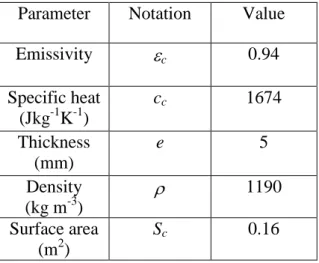
Dew mass is measured on a reference surface composed of a 400 mm x 400 mm and e = 5mm thickness Polymethylmethacrylate (PMMA; commercial name: Plexiglas) plate. The collecting area is Sc = 0.16 m2. The choice of PMMA as a standard was dictated by the
following considerations. Plexiglas is a PMMA polymer, whose long chain radiates in the near-infrared and thus behaves close to a black body above 2.5 m (the emissivity is close to unity in this wavelength region, see Table 1). PMMA is transparent to the direct sun illumination wavelength between 0.4 and 1.2 m and presents two small absorption peaks at 1.15 and 1.4 m. These peaks are responsible for some heating for direct and, to smaller extent, diffuse sun illumination. PMMA is not sensitive to UV, preventing aging when exposed; it can be sensitive to chemicals and absorb up to 3 to 4% of its weight of water. This low value does not affect our measurements. The plate is placed on an aluminum foil 12.5 m thick, and a 5 mm thick sheet of polystyrene foam for thermal insulation (Fig.1).
The following physical parameters are continuously recorded (Fig.2) on a data logger connected to a computer : plate surface temperature Tc using Type K thermocouple ( 0.1 °C),
dew mass m, air relative humidity H, air temperature Ta (TESTO sensors 0.2% for H,
0.1°C for Ta) and dew point temperature Td, wind direction and velocity V. A cup anemometer
(stalling speed: 0.5 m/s) is located at 0.1 m from the plate and 0.1 m above it. In Ajaccio, another cup anemometer (stalling speed: 0.4 m/s) is located within 3 m from the plate and 10 m above the ground. In Ajaccio and Bordeaux, low wind speed was also monitored by a hot wire anemometer located 0.1 m away from the plate and 0.1 m above it. In contrast to the cup
anemometer, which measures the wind speed parallel to the ground, the hot wire anemometer measures all wind speed components and does not exhibit a stalling speed. Its accuracy is 0.03 m/s in the range 0 – 2m/s.
All cup data have been extrapolated at z = 10 m height by using the classical logarithmic variation (see e.g. Pal Arya, 1988):
V(z) = V10 ln(z/zc)/ln(10/zc) (1)
where zc (taken here to be 0.1 m) is the roughness length.
The cloud cover data (N, in octas) is obtained from the nearest airport station (data collected every 3 hour), located within 10 km from the measurement site.
Dew (and also frost, fog and, to some extent, rain) mass m is recorded on an electronic, temperature-compensated Mettler Toledo balance (Fig.1) connected to a PC. The balance is protected up to the plate level, to avoid additional pressure from the wind. Zero is arbitrary. Note that the wind induces a force directed upwards, due to the Bernoulli pressure. A typical recording is shown in Fig.2 (time t is in UTC+1) correlating the wind events with an apparent decrease in mass. When necessary, the real mass is easily inferred from the events where wind is near zero. Typically (Fig.2), as soon as Tc < Td in the evening, the balance detects a slow
mass increase with a slope dm/dt < 5 10-2 mm/h. When in the morning Tc > Td, evaporation
takes place with a very large negative slope dm/dt. The time of dew production is determined by the time (dt) where Tc < Td (Fig.2). This is a simplification whereby water is supposed to
completely wet the substrate. Indeed, the actual temperature at which dew drops appear depends on the wetting conditions. For PMMA, it is when Tc < Td – 0.35 °C that dew starts to
form (see Section 4 below, Fitting model). The total dew mass is taken as the maximum condensed mass m0, when Tc reaches Td in the morning.
From m, it is easy to deduce the corresponding dew water precipitation h:
h (mm) = [m or m0] (g)/160. (2)
Frost is observed when Tc < 0°C. Fog occurrence is characterized by Ta Td. Rain events are
detected by the high value of m and/or its rate dm/dt which exceeds 510-2 mm/h. Both fog and rain were excluded from the dataset.
2.2. Measurement sites.
The measurement site is located in the Ajaccio Gulf at latitude 41° 55’ N and longitude 8° 48’ E, 0.5 km from the sea at 70 m elevation, on the mid-slope of a hill on a terrace 7 m from the ground. The name of the site is Vignola. The nocturnal wind regime is characterized by a NE dominant direction (1.8 m/s average) and two directions (N-W/S-W) for the diurnal dominant wind, characteristic of this Mediterranean island climate. The dew measuring device is located on a terrace and the cloud cover data are measured 10 km away at the Ajaccio airport meteorological station.
2.2.2. Grenoble
The measurement site is located north of Grenoble (45°11’ N, 5°42’ E), at a site called Polygone Scientifique. It is approximately 215 m asl and in the middle of a 10 km wide glacial valley, between the Chartreuse and Vercors mountains (2100 m maximum elevation). Two dominant wind directions, N-E and S-W, characterize the wind regime.
The first dew data were obtained on a nylon mesh (0.04 m2) of a recording Hiltner mechanical balance, between 14-08-1999 and 30-11-1999, placed 1 m above the ground. Between 25-11-1999 and 23-01-2001, the data were obtained on the equipment described in Section 2.1 above.
The cloud cover data were measured at the Le Versoud airport meteorological station (13.5 km away).
2.2.3. Bordeaux
The measurement site is located south of the Bordeaux urban area, in the town of Pessac along the urban vineyards of “Pape Clément”1
(44° 47’45’’ N, 0°39’29’’ W) approximately 17 m a.s.l. The dominant wind direction during the night (21:00 – 06:00) is SW (240°).
The cloud cover data are measured at the Merignac airport meteorological station (4.5 km away).
3. Comparison of dew data
Below we compare the dew characteristics in relation to dew yield, dew duration, dew rate, relative humidity, cloud cover, and wind speed.
1
3.1. Dew yield
The daily dew yield (h, in mm) collected overnight between day (dd -1) and (dd) are shown in Fig.3a. All diagrams in this paper are smoothed by using the LOWESS weighting algorithm (Chambers et al., 1983). The weighting factor represents roughly a portion of the data points used in the averaging procedure and is typically 20% of the total number of data. As usual, dew yield is in general at a maximum in December and at a minimum in June, the difference is mostly (but not only, as we will see below) due to the difference in night time duration. It should be noted, however, that the oscillations in Ajaccio are more damped than in Grenoble or Bordeaux. Grenoble exhibits the highest seasonal variation. There are different possible causes to explain this oscillation behavior; the more obvious being night duration, wind regime, cloud cover and available humidity - all parameters that we analyze below.
It is also interesting to consider the dew yield compared over the same one-year period. The mean yield for a one-year period (see below, Table 2) is larger in Ajaccio ( 0.070 mm) than in Bordeaux (0.046 mm) and in Grenoble (0.036 mm).
The cumulated dew yield takes into account the frequency of dew events in addition to the dew yield. Fig. 3b shows the cumulated dew volumes over one year. The production of dew water is more regular in Ajaccio. It is interesting to note that the cumulated yield is larger in Bordeaux (9.8 mm) than in Ajaccio (8.43 mm), although the mean dew rate is smaller. This observation is due to the greater number of (smaller) dew yield events in Bordeaux. Grenoble gives the smallest value: 3.95 mm.
3.2. Dew duration
The time duration (dt) where dew forms, as defined in Section 2.1, is plotted in Fig. 4. For all locations it shows a periodicity in phase with the seasons, with amplitude ranging, as for the dew yield, from Grenoble (the largest) to Ajaccio (the smallest). This result, which seems obvious, could mean that the dew rate is nearly constant over the year. We note, however, some phase shifts indicating that the dew rate evolution, analyzed in the next section, is not simple.
The dew rate is presented in Fig. 5 for the three locations. In Bordeaux, the dew rate is nearly constant, which means that the seasonal variation in dew yield is only due to night duration. In Grenoble, there is a seasonal variation with a maximum in winter. In contrast, in Ajaccio, the dew rate is at a maximum in summer.
The oscillation behavior can be related e.g. to the seasonal variation of wind, relative humidity and cloud cover. In Bordeaux, the seasonal variation of these parameters nearly compensates each other. The shorter night duration and the lower relative humidity are balanced by less cloud cover, i.e. more radiative cooling energy (see below Section 3.5). For statistical purposes, the one-year mean dew rates are reported in Table 2. The mean dew rate is larger in Ajaccio ( 0.014 mm/hour) than in Bordeaux (0.0053 mm/hour) and Grenoble (0.0039 mm/hour).
3.4. Relative humidity – dew temperature
The relative humidity is a difficult parameter to assess as it is very much a function of air temperature. However, it appears to be a key parameter for dew formation. As the cooling effect of the condenser surface cannot exceed a few degrees below air temperature (condenser temperature is remarkably parallel to air temperature, see Fig.2 and Fig. 12 below), a high relative humidity is needed to observe dew. This situation is more favorably met during the night and in the early morning where air temperature is coolest and thus the relative humidity is highest. In order to illustrate this point, we plot in Fig. 6 the difference Td - Ta as a function
of relative humidity H for different air temperatures. If we consider that the condenser provides an average cooling effect of 5 °C, the threshold in relative humidity is 67% for air at -10°C and 76 % for air at 40 °C. The conclusion is that this threshold does not vary very much with air temperature and is of the order of 70% for a cooling effect Tc - Ta = - 5°C.
The occurrence of dew in different places (not the dew yield, which depends on many other parameters) can be quantified by the ability of a surface to reach the dew temperature. According to the remarks above, this condition determines a threshold in relative humidity. The relative humidity H in Ajaccio, Grenoble and Bordeaux exhibits maxima of nearly 100 %, corresponding to Td - Ta = 0, a situation encountered with either rain, fog or dew. The
minima correspond mostly to the warmest hour of the day (and the summer time). We therefore chose in Fig. 7 to consider the average values as obtained by weighting the data with the weighting factor of 10%. Grenoble (1-year average: 71.5%) and Ajaccio (1-year average: 68.6 %) exhibit about the same relative humidity level. Relative humidity is greater in
Bordeaux, as expected from an oceanic climate (1-year average: 78.0%). Dew in Bordeaux is thus expected more frequently – which is effectively the case, as outlined in Section 3.1.
3.5. Cloud cover
Another parameter of importance is the cloud cover N, which is a rough, but convenient, measurement of the cooling energy. Figure 8 contains the cloud cover Nm averaged over the
time dt where dew forms. Oscillations in phase with the seasons are also found, with the lowest amount of cloud cover in summer. The oscillations are less marked in Bordeaux (where the cloud cover exhibits the largest values). The observation (see above, Section 3.3) of a nearly constant dew rate in Bordeaux is therefore due to the compensation in summer of both shorter night duration and (slightly) lower relative humidity, by less cloud cover, i.e. more radiative cooling energy.
It should be noted that dew forms in all sites when the cloud cover is not at the lowest values (mean value: 3.5). This observation is associated with the need for high relative humidity to observe dew. Ajaccio has the lowest cloud cover (mean valueN = 3.2 during all periods, m
m
N = 3.1 for a 1-year average, see Table2) and Bordeaux the highest (mean value N = 3.8 m
during all periods, N = 3.9 on a 1-year average, see Table2). Grenoble exhibits the medium m
value (mean valueN = 3.5 during all periods, m N = 3.4 on a 1-year average, see Table 2). m
The reason why dew yield in Bordeaux is larger than in Grenoble, although cloud cover is higher, corresponds to the high relative humidity in Bordeaux, which cancels the effect of highest Nm. In addition, Grenoble lies in the bottom of an alpine valley where the atmospheric
transmittency is not very high because of atmospheric pollution, even though the cloud cover is low.
3.6. Wind speed
Figure 9 compares the average wind during the dew events (dt). There is a striking difference between the sites. In Bordeaux and Grenoble dew forms with a near zero wind velocity (1-year average from Table 2: Bordeaux, 0.13 m/s; Grenoble: 0.22 m/s), whereas in Ajaccio the wind speed is more important by a factor of about 10 (1-year average from Table 2: 1.95 m/s).
This observation highlights the peculiarities of islands, where a nocturnal thermal breeze is generally present.
Concerning Bordeaux, the hot wire anemometer measures the air flows in all directions - not only flows parallel to the ground as does a cup anemometer. The value found by the hot wire anemometer is nearly constant no matter the season, with an average of 0.51 m/s, and shows that the thermal exchange is mostly due to the air motion next to the ground and the condensing plate.
In an attempt to determine a correlation between the cup and the hot wire anemometer, we compared Vc and Vf (data from 07-04-2002 to 14-01-2003) in Fig. 10. These data correspond
to all measurements, day and night. As expected,, the correlation is non-linear. The relation between Vc and Vf can be fitted to a quadratic function:
Vc = V0+(dVc /dVf )0* Vf +
2 1
(d2Vc /dVf 2)0Vf 2 . (3)
The values for the coefficients are V0 = (0.588 ± 0.002) m/s; (dVc/dVf)0 = 0.941 ± 0.009;
0.5(d2Vc/dVf2)0 = (0.103 ± 0.005) s/m. These parameter values can be interpreted at small wind
speed values as the measurement of the superposition of a wind flow parallel to the ground (the linear slope at origin (dVc/dVf)0 is unity within the uncertainty) and a “noise” of
amplitude 0.6 m/s. This contribution, which is of the order of the average value measured during dew events ( 0.5 m/s), corresponds to the local convective air flows.
3.7. Synthesis
The mean dew yield in Ajaccio (island) is nearly two times larger than in Grenoble (continental), and 50% larger than in Bordeaux (coastal). Such large differences do not stem from the dew formation time, which is longer in Grenoble than in Bordeaux, and in turn longer than in Ajaccio. This difference is visible in the dew rates, nearly 4 times greater in Ajaccio than in Grenoble and 2.5 times greater than in Bordeaux. We note that dew yield seasonal variation is very weak in Bordeaux, and that the maximum dew rate is observed in
summer in Ajaccio and in winter in Grenoble. This high dew rate is not related to wind, as
Ajaccio shows a mean wind speed during dew formation higher by a factor of 5 than Grenoble, and by a factor of 15 compared to Bordeaux. It is neither due to the cloud cover influence, as Ajaccio and Grenoble have nearly the same values ( 1-year average, Ajaccio: 3.1, Grenoble = 3.4, respectively). Bordeaux exhibits a somewhat larger cloud cover value (1-year average: 3.9). Another factor could be relative humidity, which measures the occurrence
of dew (but not its magnitude). However, relative humidity is the highest in Bordeaux (which explains the higher number of dew days) and of nearly the same amplitude in Ajaccio and in Grenoble. The reason for such a high dew rate in Ajaccio can be tentatively explained in terms of better atmospheric transparency. Our measurements show that the far-infrared radiation issued from the sky in Ajaccio is of the order of -150 Wm-2, a value noticeably larger than commonly found (-100 Wm-2). This interpretation in terms of larger atmospheric transparency in Ajaccio is in agreement with the low transmittency in the Grenoble valley and the higher cloud cover in Bordeaux.
The cumulated dew yield – which is the important parameter for dew harvesting – is lowest in Grenoble ( 4 mm), which shows a cumulated yield less than half of Ajaccio, with a daily rate and a lower number of dew days. The cumulated dew is the most important in Bordeaux ( 10 mm), with Ajaccio showing a smaller cumulated yield (8.5 mm). As the average daily yield of Ajaccio is larger than that of Bordeaux, this result appears as a paradox. However, the lower daily dew accumulation rate of Bordeaux is overcompensated by a much larger number of dew days (by nearly a factor of two for Ajaccio and Grenoble).
The lower number of dew days in Ajaccio, when compared to Bordeaux, is due to both the lower relative humidity and higher wind speed that hampers dew formation. Note that when the wind influence is reduced in special condensing surface configurations, the number of dew events and the cumulated dew yield in Ajaccio is increased by at least 50 % (Muselli et al., 2002).
4. Fitting model
In order to fit and predict dew formation from simple meteorological measurements, we use a numerical model (Nikolayev et al., 2001) based on the models by Pedro and Gillespie (1982) and Nikolayev et al. (1996), valid during the night period.
The heat balance equation for the condenser is :
(dTc/dt)(Mcc+mcw) = Ri+Rhe+Rcond (4)
where Tc is the condenser's temperature, M (= eSc) and m are the masses of the condenser
and condensed water, respectively, with the condenser density. cc and cw are the specific
heats of the material of the condenser and water, and t is time. Hereafter, SI units are used for all values except temperature, which is expressed in Celsius degrees. The variables in the right-hand side represent the different physical processes involved in the heat energy coming
to or leaving the condenser surface: Ri is the irradiation, Rhe is the heat exchange with the
surrounding air, and Rcond is the energy gain due to the latent heat of the condensation (L per
unit mass). Thus
Rcond =L(dm/dt) . (5)
The convective heat exchange term can be expressed in the usual form as
Rhe =Sca(Ta – Tc), (6)
where a is a heat transfer coefficient and Sc is the condenser's surface area. The parameter a
relates to the width of the aerodynamical boundary air layer and thus depends on the wind speed V (the conditions of forced convection heat transfer are assumed):
a = kf (V/D)1/2 . (7)
Here the numerical factor f = 4WK-1m-2s1/2 is empirical; its value is from Pedro and Gillespie (1982) and corresponds to a flow parallel to a plane sheet of size D = Sc1/2. We introduced a
correction coefficient, k, that depends on the relative position of the condenser with respect to the device measuring the wind velocity, and on the particular air flow conditions.
The total irradiation term from Eq. 4 can be divided into two parts:
Ri = Rl - Rc . (8)
Rl is the incoming long-wave irradiation and Rc is the outgoing irradiation of the condenser. It
can be represented by
Rc = Scc(Tc+273)4 , (9)
where is the Stephan-Boltzmann constant and c is the emissivity of the condenser. The
long-wave radiation term is given by Pedro and Gillespie (1982) and Campbell (1977):
Rl = Sccs(Tc+273)4 , (10)
where s is the emissivity of the sky, which depends on the ambient temperature Ta and on the
cloud cover N measured on a scale 0-8 (octas):
s = s0 + (N/8) [1-s0 -8/(Ta+273)] (11)
where s0 = 0.72+0.005Ta. This is a simplified version of the irradiation energy that neglects
the effects on sky transmittency of aerosols, green house gases, etc. As N is usually obtained on a 3 hour observation basis, a linear interpolation is performed to calculate it for smaller (15 minute) time intervals.
The equation for m represents the condensation rate:
dm/dt = Scb[psat (Td) - pc(Tc)], if positive, (12)
Here psat(T) is the saturation pressure at given temperature T. The dew point temperature Td
can be determined from the equation
Hpsat(Ta)=psat(Td) , (13)
pc(Tc) is the vapor pressure over the condenser at the temperature Tc at which condensation on
its surface begins. Generally speaking, pc(Tc) does not coincide with psat(Tc) and depends on
the degree of wettability of the surface by water (see Beysens, 1995). When the surface is wetted, the condensation on it can begin even when T>Td. We assume that it begins when T =
Td-T0, i.e. pc(Tc) = psat(Tc+T0), where T0<0 is another fitting parameter that depends on the
wetting conditions of the condenser surface and that does not vary with time. We take T0 =
-0.35°C in the following calculations. Equation 13 assumes the absence of evaporation of the already condensed water as if it were removed from the condenser as soon as condensation has stopped.
The value of the mass transfer coefficient b is proportional to a from Eq.7:
b = 0.656 ga/(pca) , (14)
where p is the atmospheric pressure (assumed constant) and ca is the specific heat of air. This
expression, as well as the numerical factor, comes from the calculations by Pedro and Gillespie (1982). We added another adjustable time-independent parameter, g, to account for the particular air flow conditions around the condenser.
Equations (4) and (12) form a set of ordinary differential equations that are integrated for each night of observations separately. The initial time for the calculations is chosen somewhere after sunset, before the condensation starts, so that initially m = 0. The end time for the calculation should be chosen before sunrise.
The purpose of the fitting procedure is to obtain the values for two parameters k and g. The least squares method was used for the fitting. The fitting is performed in two stages. First, a value for g is guessed. This value directly influences the mass of the condensed water m. Since m << M, the influence of the m evolution (and g) on Tc is very small. Therefore, the
error in g has very little effect on the Tc calculation. For the same reason we can neglect the
difference between the condensation and sublimation latent heat in Eq.5. Therefore the frost mass can be assessed by the same procedure as the dew amount.
By minimizing the difference between Tc and Tc, exp we obtain a value for k. This value is used
at the second stage where we minimize the difference between m and mexp by adjusting g. The
value of Tc, exp at the initial moment of time is used as the initial condition for Eq.6. (The
Organization for Dew Utilization (OPUR, http://www.opur.u-bordeaux.fr) together with examples of the data files and other documentation.)
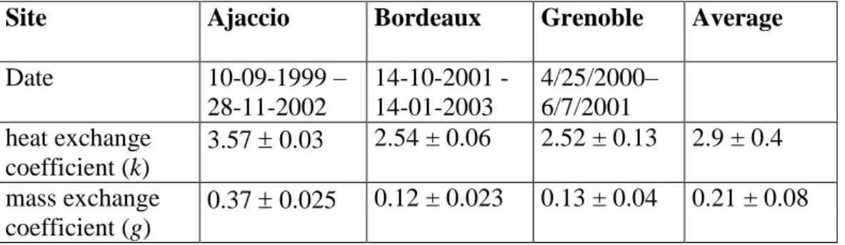
The results of the analysis of the data from Ajaccio, Bordeaux and Grenoble are presented in Fig.11 and Table 3. The average values do not appreciably vary with time, in contrast to the data analyzed above (dew yields h, condensation time dt, N, V, etc.). In addition, the values found in these three sites are in relatively good agreement, with however somewhat larger values for Ajaccio. We attribute this deviation to the fact that the model is not perfect and open for improvement. This result demonstrates that both the fitting function and the choice of k and g as adjustment parameters are good. Both k and g deviate from unity, with average values k 3 and g 0.2.
A fit to data calculated with k = 3.59 and g = 0.434 is presented in Fig.12. The condensation begins at about 23h and ends at about 4h30. During this interval of time, Tc stays below the
condensation temperature Td – T0. The condenser temperature stays several degrees cooler
than air due to the radiation losses. The simulated temperature stays close to Tc, exp during all
the period until the end of dew formation, the variance of Tc - Texp being less than 0.34°C.
The fit to m is equally quite good.
A fit failure can be due to both the high wind speed necessary for the onset of the cup anemometers (V < 0.5 m/s result in V = 0) and an error in the correlation (Eq. 7) for the convective heat transfer coefficient. According to (Eq. 7), there is no convective heat exchange when V = 0, which is apparently wrong (in Bordeaux, with the hot wire anemometer, there is always noise in the order 0.5 m/s, see Fig. 9). This inconsistency appears because Eq. 7 is only valid when a mean wind can be resolved by the cup anemometer. When
V is small, the turbulence becomes the dominant mechanism of the convective heat transfer.
This shows the necessity to correct Eq. 7 in order to account for the turbulence and to have more sensitive V measurement. An approximate way could be to impose the average value (0.5 m/s) found during dew formation by the hot wire anemometer.
We also recognize that strong air motion caused by frequently varying wind velocity over such a condenser sometimes creates spurious balance oscillations that can manifest themselves as an artificial increase or decrease of the measured mass.
5. Conclusion
A precise prediction of dew occurrence and dew yield is still a challenge when only simple meteorological data are available. This prediction is, however, of importance for
agriculturalists and, more generally, scientists or individuals requiring dew water yield data for a given application such as, for example, dew water harvesting. In one of the simplest situations where the surface on which dew condenses is flat and well characterized, we developed an algorithm and a set of PC software to predict the amount of condensed water on the condenser plate (and the condenser temperature during night). This software was verified against the experimental data in Ajaccio, Bordeaux and Grenoble. As a rule, the variance of the difference between the measured and simulated temperatures of the condenser plate did not exceed 0.5 °C. The model has two adjustable parameters k (heat exchange coefficient) and
g (mass exchange coefficient) that depend on the position and structure of the condenser.
They are shown to be independent of time and the values are roughly the same in all sites, within the uncertainties.
However, this model has some limitations. It does not work well when the wind is weak (less than ~1m/s) for a long period of time and cannot calculate the actual energy budget between solar and terrestrial or long wave radiation (it uses cloud cover to estimate the radiation energy balance). A simple improvement would be to use a background turbulent wind velocity of about 0.6 m/s as outlined in Section 3.6.
On a more particular note, the observations highlight the high dew rate in Ajaccio, despite the high wind speeds, and the large cumulated dew yield in Bordeaux. The dew rate seasonal variation is not systematically linked to the seasonal variation of the night duration: it is negligible in Bordeaux, at a maximum in Ajaccio during summer, and at a maximum in Grenoble in winter. It proves the importance of the local variation of humidity, a parameter as important as the radiative cooling energy.
Acknowledgments
References
Beysens D., 1995. The formation of dew. Atmospheric Research 39: 215-237.
Beysens, D., Milimouk, I., Nikolayev, V., Muselli, M., Marcillat, J., 2003. Using radiative cooling to condense atmospheric vapor: a study to improve water yield, J Hydrology 276: 1-11.
Broza, M.,1979. Dew, fog and hygroscopic food as a source of water for desert arthropods. J. Arid Environ 2: 43-49.
Campbell, G.S., 1977. An Introduction to Environmental Biophysics, Springer Verlag, New-York.
Chambers, J. M., Cleveland, W. S., Kleiner, B., and Tukey, P. A., 1983. Graphical Methods for Data Analysis. Duxbury Press, Boston.
Muselli, M., Beysens, D., Marcillat, J., Milimouk, I., Nilsson, T., Louche, A., 2002. Dew water collector for potable water in Ajaccio (Corsica Island, France). Atmos. Res. 64: 297 – 312.
Nikolayev, V.S., Beysens D., Gioda A., Milimouk I., Katiushin E., Morel J.-P., 1996. Water recovery from dew. J. Hydrology 182: 19-35.
Nikolayev, V.S., Beysens, D., Muselli, M., 2001. A Computer Model for Assessing Dew/Frost Surface Deposition. Proceedings of the 2nd International Conference on Fog and Fog Collection, St John’s (Canada), July 16-20, 2001, Eds. R. S. Schemenauer and H. Puxbaum, IDRC, p.333 – 336.
(See http://www.opur.u-bordeaux.fr/Data%20Processing/FitDew-ST%20JOHN.pdf)
Pal Arya, S., 1988. Introduction to Micrometeorology. Academic Press, Inc., San Diego.
Monteith J.L. and Unsworth M.H., 1990. Principles of Environmental Physics (2nd edition). Routledge, Chapman and Hall, Inc., New-York.
Pedro, M.J. and T.J. Gillespie, 1982. Estimating dew duration. I. Utilizing micrometeorological data. Agric. Meteorol. 25: 283-296.
Steinberger, Y., Loboda, I., Garner, W., 1989. The influence of autumn dewfall on spatial and temporal distribution of nematodes in the desert ecosystem. J. Arid Environ. 16: 177–183.
Figure Captions
Fig. 1. Dew measurement setup (Ajaccio). B: balance + Plexiglas plate with surface thermocouple; Vc: cup anemometer; Vf: hot wire anemometer; H: hygrometer and air temperature sensor.
Fig. 2. Typical experimental data recorded at the Bordeaux station (June 30th, 2002 to July, 1st, 2002). The cloud cover is taken from the nearest airport (Merignac). dt is the time where
Tc < Td . (for parameter definitions, see text.)
Fig. 3. Evolution of dew yield (mm). (a) daily dew yield. The curves (Ajaccio: dotted line; Grenoble and Bordeaux: full lines) are data weighted by 20% (see text). Negative bars: frost events (Grenoble and Bordeaux; no frost detected in Ajaccio). (b) cumulated dew yield (mm) evolution during a 1-year period.
Fig. 4. Dew duration time (20 % weighted, see text) in Ajaccio (dashed line), in Grenoble and Bordeaux (continuous line).
Fig. 5. Time dependence of the dew rate (mm/h, weighted 20%, see text). Ajaccio: dashed line; Grenoble and Bordeaux: continuous line.
Fig. 6. Difference Td – Ta versus relative humidity H (semi-log plot). The lines are for Ta =
-10, 0, -10, 20, 30, 40 (in °C). Warmer air needs only slightly more relative humidity to make dew. For a threshold Ta-Td =-5 °C, the threshold is 67% for air at -10°C and 76 % for air at 40
°C .
Fig. 7. Evolution of the mean relative humidity. The curves correspond to data weighted by 20% (see text). Grenoble: continuous, grey; Bordeaux: continuous, black; Ajaccio: dotted, black.
Fig. 8. Evolution of the average cloud cover (octas) corresponding to dew events. Data have been weighted by 20% (see text). Ajaccio: dotted line; Grenoble: grey; Bordeaux: black.
Fig. 9. Wind speed averaged over the dew duration time dt with respect to time (Vc: cup
anemometer at 10 m height, continuous lines; Vf: hot wire anemometer at 1 m height, dotted
line). The data have been smoothed with the following weighting factors (see text ): Ajaccio:
Vc , 20%; Grenoble: Vc , 8%; Bordeaux: Vc , 6%, Vf , 10%.
Fig. 10. Correlation of the wind speed measured by the hotwire (Vf) anemometer and that of
the cup anemometer (Vc) in Bordeaux (07-04-2002 to 14-01-2003).
Fig. 11. The thermal (k: black dots) and mass (g: open squares) coupling parameters in (a) Grenoble, (b) Ajaccio and (c) Bordeaux.
Fig. 12. The data fit for the night of January, 10-11, 2000, Ajaccio. The time format is dd:hh:mm:ss.
Tables and Tables Captions
Table 1. Condenser parameters used for the calculations. The condenser plate was made of Plexiglas (PMMA).
Parameter Notation Value
Emissivity c 0.94 Specific heat (Jkg-1K-1) cc 1674 Thickness (mm) e 5 Density (kg m-3) 1190 Surface area (m2) Sc 0.16
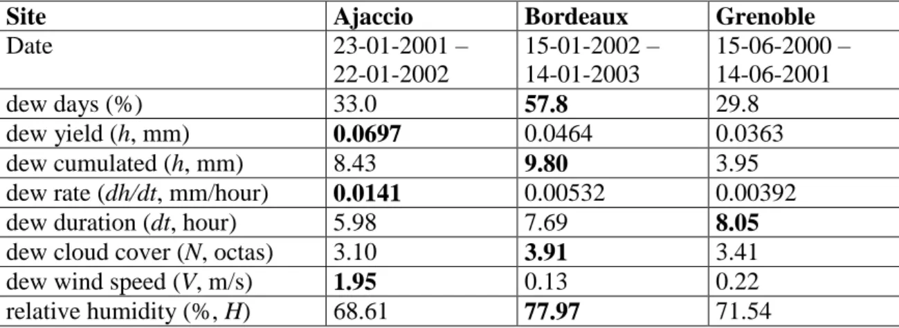
Site Ajaccio Bordeaux Grenoble Date 23-01-2001 – 22-01-2002 15-01-2002 – 14-01-2003 15-06-2000 – 14-06-2001 dew days (%) 33.0 57.8 29.8 dew yield (h, mm) 0.0697 0.0464 0.0363 dew cumulated (h, mm) 8.43 9.80 3.95 dew rate (dh/dt, mm/hour) 0.0141 0.00532 0.00392 dew duration (dt, hour) 5.98 7.69 8.05
dew cloud cover (N, octas) 3.10 3.91 3.41 dew wind speed (V, m/s) 1.95 0.13 0.22 relative humidity (%, H) 68.61 77.97 71.54
Table 2. Comparison of dew and dew-related characteristics averaged over a 1-year period. The maximum values are highlighted.
Site Ajaccio Bordeaux Grenoble Average Date 10-09-1999 – 28-11-2002 14-10-2001 - 14-01-2003 4/25/2000– 6/7/2001 heat exchange coefficient (k) 3.57 0.03 2.54 ± 0.06 2.52 ± 0.13 2.9 ± 0.4 mass exchange coefficient (g) 0.37 0.025 0.12 ± 0.023 0.13 ± 0.04 0.21 ± 0.08
Table 3. Heat and mass exchange coefficients from the fit of condenser temperature Tc and
Figures